A Bimodal Model Based on Truncation Positive Normal with Application to Height Data

Abstract

In this work, we propose a new bimodal distribution with support in the real line. We obtain some properties of the model, such as moments, quantiles, and mode, among others. The computational implementation of the model is presented in the tpn package of the software R. We perform a simulation study in order to assess the properties of the maximum likelihood estimators in finite samples. Finally, we present an application to a bimodal data set, where our proposal is compared with other models in the literature.

1. Introduction

Describing a phenomenon by a probability distribution is very useful because of the properties associated with it: expectation, shape, range, etc. However, this description can be difficult when a phenomenon (in practice, an observed dataset) is bimodal, which occurs commonly in areas like astrophysics, ecology and genetics; see [1,2,3], respectively. The first approach to fit a bimodal data is using a mixture of two unimodal distributions, for instance, a mixture of gaussian distributions; see [4]. The main disadvantage of this procedure is the non-identifiability of the proposed mixture model. The second and the most workable practical approach is to use distributions which already have bimodal properties. Because of these properties, there is an increasing interest to derive bimodal distributions in the literature: refs. [5,6] presented extensions of the skew-normal, ref. [7] proposed a generalization of the Burr type X distribution and [8] derived an extension of the sinh Cauchy distribution. In this paper, we will discuss an extension of the half normal distribution proposed by [9], the truncated positive normal (tpn) model. The probability density function (pdf) for the tpn model is given by

$$f(x;\sigma ,\lambda )=\frac{1}{\sigma \mathsf{\Phi }\left(\lambda \right)}\varphi \left(\frac{x}{\sigma }-\lambda \right),x,\sigma \in {\mathsf{ℝ}}_{+},\lambda \in \mathsf{ℝ},$$

where $\sigma$ and $\lambda$ are the scale and shape parameters, respectively, and $\varphi (·)$ and $\mathsf{\Phi }(·)$ are the pdf and cumulative distribution function (cdf), respectively, of the standard normal distribution. The corresponding cdf of the tpn model is

$$F_X(x;\sigma ,\lambda )=\frac{\mathsf{\Phi }(\frac{x}{\sigma }-\lambda )+\mathsf{\Phi }\left(\lambda \right)-1}{\mathsf{\Phi }\left(\lambda \right)}.$$

Note that the cdf above has a closed-form expression, which is useful for generating random data besides defining quantiles. For more properties of the tpn model, see [9]. The restriction to positive values is a limitation of the tpn model. To overcome this limitation, the chief goal of this paper is to derive an extension of the tpn model which has support in the real line. We describe in detail the model, studying its main properties and related functions. Moreover, we show analytically the regions in which the model is unimodal and bimodal, and such regions depend only on one parameter.

The paper is organized as follows. In Section 2, we derive an extension of the tpn with support in the real line and study some properties of the distribution. The inference for parameter estimation in the proposed model and computational aspects are presented in Section 3. In Section 4, we perform a simulation study to evaluate the parameter estimation in finite samples. An application to real data is discussed in Section 5. Finally, conclusions are given in Section 6.

2. A Bimodal Truncation Positive Normal Distribution

In this section, we present the stochastic representation for the bimodal truncation positive normal (btpn) distribution and some properties, such as its pdf and its cdf. We also discuss some particular cases of the model.

2.1. Stochastic Representation, pdf and cdf

Let T be a discrete random variable such as

$$T=\{\begin{array}{cc}-(1+ϵ)\hfill & ,\mathrm{with} \mathrm{probability} (1+ϵ)/2\\ 1-ϵ\hfill & ,\mathrm{with} \mathrm{probability} (1-ϵ)/2\end{array},$$

where $ϵ\in (-1,1)$. If $Z\sim \mathrm{tpn}(\sigma ,\lambda )$, independent from T, then we define a new random variable given by $X=ZT$. We say that X follows a btpn distribution.

Proposition 1.

The pdf for the btpn distribution is given by

$$f(x;\sigma ,\lambda ,ϵ)=\{\begin{array}{cc}\frac{\varphi \left(\frac{x}{\sigma (1+ϵ)}+\lambda \right)}{2\sigma \mathsf{\Phi }\left(\lambda \right)}\hfill & ,if x<0\\ \frac{\varphi \left(\frac{x}{\sigma (1-ϵ)}-\lambda \right)}{2\sigma \mathsf{\Phi }\left(\lambda \right)}\hfill & ,if x\ge 0\end{array},$$

where $\sigma >0,\lambda \in \mathbb{R}$ and $ϵ\in (-1,1)$.

Proof. 

If $x<0$, then the cdf for X is

$$\begin{array}{ccc}\hfill F_X\left(x\right)& =& P(X\le x)=\frac{(1+ϵ)}{2}P\left(z\ge \frac{-x}{1+ϵ}\right)=\frac{(1+ϵ)}{2}\left[1-P\left(z\le \frac{-x}{1+ϵ}\right)\right]\hfill \\ & =& \frac{(1+ϵ)}{2}\left[1-F_Z\left(\frac{-x}{1+ϵ}\right)\right].\hfill \end{array}$$

Deriving the last expression in relation to x, we have

$$f_X\left(x\right)=\frac{(1+ϵ)}{2}\left[-f_Z\left(\frac{-x}{1+ϵ}\right)\frac{-1}{(1+ϵ)}\right]=\frac{1}{2}\left[\frac{1}{\sigma \mathsf{\Phi }\left(\lambda \right)}\varphi \left(\frac{\frac{-x}{(1+ϵ)}}{\sigma }-\lambda \right)\right]=\frac{\varphi \left(\frac{x}{\sigma (1+ϵ)}+\lambda \right)}{2\sigma \mathsf{\Phi }\left(\lambda \right)}.$$

A similar routine calculation shows that for $x\ge 0$, we have that

$$f_X\left(x\right)=\frac{\varphi \left(\frac{x}{\sigma (1-ϵ)}-\lambda \right)}{2\sigma \mathsf{\Phi }\left(\lambda \right)},$$

completing the proof. □

Figure 1 shows the pdf function for the btpn model with different combination of parameters. Note that the model can assume different shapes, including unimodal, bimodal, symmetric and asymmetric.

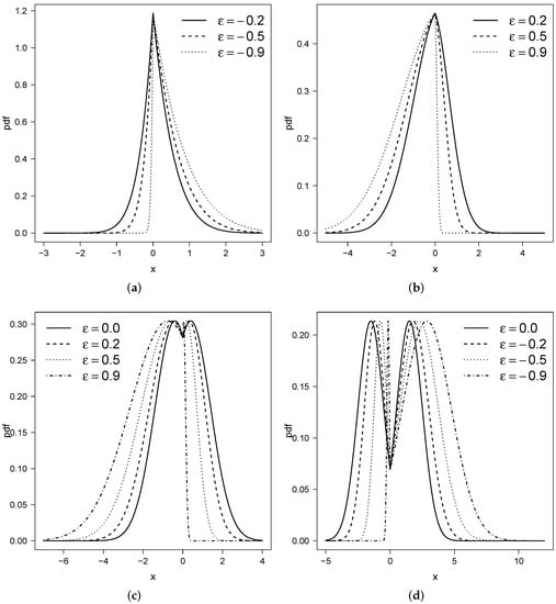
Figure 1. Pdf for btpn$(\sigma =1,\lambda ,ϵ)$ with different fixed values for $\lambda$ and varying $ϵ$: (a) $\lambda =-2$; (b) $\lambda =-0.2$; (c) $\lambda =0.4$ and; (d) $\lambda =1.5$.

Proposition 2.

The cdf of $X\sim btpn(\sigma ,\lambda ,ϵ)$ is given by

$$F_X\left(x\right)=\{\begin{array}{cc}\frac{(1+ϵ)}{2\mathsf{\Phi }\left(\lambda \right)}\mathsf{\Phi }\left(\frac{x}{\sigma (1+ϵ)}+\lambda \right)\hfill & ,if x\le 0\\ \frac{(1-ϵ)}{2\mathsf{\Phi }\left(\lambda \right)}\left[\mathsf{\Phi }\left(\frac{x}{\sigma (1-ϵ)}-\lambda \right)+\mathsf{\Phi }\left(\lambda \right)-1\right]\hfill & ,if x\ge 0\end{array}$$

Proof. 

It is immediate from the last proof. □

Proposition 3.

Let there be $X\sim btpn(\sigma ,\lambda ,ϵ)$. Its quantile function is given by

$$Q_X\left(p\right)=F_X^{-1}\left(p\right)=\{\begin{array}{cc}\sigma (1+ϵ)\left[{\mathsf{\Phi }}^{-1}\left(\frac{2p\mathsf{\Phi }\left(\lambda \right)}{1+ϵ}\right)-\lambda \right]\hfill & ,if 0<p\le \frac{1+ϵ}{2}\hfill \\ \sigma (1-ϵ)\left[{\mathsf{\Phi }}^{-1}\left(\frac{2p\mathsf{\Phi }\left(\lambda \right)}{1-ϵ}-\mathsf{\Phi }\left(\lambda \right)+1\right)+\lambda \right]\hfill & ,if \frac{1+ϵ}{2}<p<1\hfill \end{array}$$

Proof. 

It is immediate from inverting the cdf for the btpn distribution given in Proposition 2. □

Corollary 1.

The median for $X\sim btpn(\sigma ,\lambda ,ϵ)$ is given by

$$Me\left(X\right)=\{\begin{array}{cc}\sigma (1+ϵ)\left[{\mathsf{\Phi }}^{-1}\left(\frac{\mathsf{\Phi }\left(\lambda \right)}{1+ϵ}\right)-\lambda \right]\hfill & ,if ϵ\ge 0\hfill \\ \sigma (1-ϵ)\left[{\mathsf{\Phi }}^{-1}\left(\frac{ϵ\mathsf{\Phi }\left(\lambda \right)}{(1-ϵ)}+1\right)+\lambda \right]\hfill & ,if ϵ<0.\hfill \end{array}$$

Corollary 2.

The median for $X\sim btpn(\sigma ,\lambda ,ϵ)$ is $<0$, $=0$ and $>0$ if ϵ is $>0$, $=0$ and $<0$, respectively.

2.2. Moments and Moment-Generating Function

The following proposition presents the central moments of the btpn distribution.

Proposition 4.

Let $X\sim btpn(\sigma ,\lambda ,ϵ)$. The r-th central moment of X is given by

$$E\left(X^r\right)=\frac{{\sigma }^r}{2\sqrt{2\pi }\mathsf{\Phi }\left(\lambda \right)}\left[{(-1)}^r{(1+ϵ)}^{r+1}+{(1-ϵ)}^{r+1}\right]\sum _{k=0}^r\left(\genfrac{}{}{0pt}{}{r}{k}\right){\lambda }^{r-k}{\left(2\right)}^{(k-1)/2}\Gamma (k+1)/2,{\lambda }^2/2),$$

where $\Gamma (a,b)={\int }_b^{+\infty }{t}^{a-1}{e}^{-t}dt$ is the upper incomplete gamma function.

Proof. 

Note that $E\left(X^r\right)=E_1\left(X^r\right)+E_2\left(X^r\right)$, where $E_1\left(X^r\right)={\int }_{-\infty }^0{x}^{r}f\left(x\right)dx$ and $E_2\left(X^r\right)={\int }_0^{+\infty }{x}^{r}f\left(x\right)dx$. For the first term, we perform the change of variable $u=\frac{-x}{\sigma (1+ϵ)}-\lambda$. With this,

$$\begin{array}{ccc}\hfill E_1\left(X^r\right)& =& {\int }_{-\infty }^0\frac{x^r}{2\sigma (1+ϵ)}\varphi \left(\frac{-x}{\sigma (1+ϵ)}-\lambda \right)dx\hfill \\ & =& \frac{{(-\sigma )}^r{(1+ϵ)}^{(r+1)}}{2\mathsf{\Phi }\left(\lambda \right)}{\int }_{-\lambda }^{\infty }{(u+\lambda )}^r\varphi \left(u\right)du.\hfill \end{array}$$

Using the binomial theorem and the change of variable $t=u^2/2$ in the last expression, we obtain

$$\begin{array}{ccc}\hfill E_1\left(X^r\right)& =& \frac{{(-\sigma )}^r{(1+ϵ)}^{(r+1)}}{2\sqrt{2\pi }\mathsf{\Phi }\left(\lambda \right)}\sum _{k=0}^r\left(\genfrac{}{}{0pt}{}{r}{k}\right){\lambda }^{r-k}{\int }_{-\lambda }^{\infty }{u}^k{e}^{-u^2/2}du,\hfill \\ & =& \frac{{(-\sigma )}^r{(1+ϵ)}^{(r+1)}}{2\sqrt{2\pi }\mathsf{\Phi }\left(\lambda \right)}\sum _{k=0}^r\left(\genfrac{}{}{0pt}{}{r}{k}\right){\lambda }^{r-k}{2}^{(k-1)/2}{\int }_{{\lambda }^2/2}^{\infty }{t}^{(k-1)/2}{e}^{-t}dt,\hfill \end{array}$$

Note that the last integral corresponds to $\Gamma ((k+1)/2,{\lambda }^2/2)$.

On the other hand, for $E_2\left(X^r\right)$, we perform the change of variable $u=\frac{x}{\sigma (1-ϵ)}-\lambda$, obtaining

$$\begin{array}{ccc}\hfill E_2\left(X^r\right)& =& {\int }_0^{\infty }\frac{x^r}{2\sigma (1-ϵ)}\varphi \left(\frac{x}{\sigma (1-ϵ)}-\lambda \right)dx\hfill \\ & =& \frac{{\sigma }^r{(1-ϵ)}^{(r+1)}}{2\mathsf{\Phi }\left(\lambda \right)}{\int }_{-\lambda }^{\infty }{(u+\lambda )}^r\varphi \left(u\right)du.\hfill \end{array}$$

Using the same routine calculation, we obtain

$$E_2\left(X^r\right)=\frac{{\sigma }^r{(1-ϵ)}^{(r+1)}}{2\sqrt{2\pi }\mathsf{\Phi }\left(\lambda \right)}\sum _{k=0}^r\left(\genfrac{}{}{0pt}{}{r}{k}\right){\lambda }^{r-k}{2}^{(k-1)/2}{\int }_{{\lambda }^2/2}^{\infty }{t}^{(k-1)/2}{e}^{-t}dt,$$

where again the last integral corresponds to $\Gamma ((k+1)/2,{\lambda }^2/2)$. The final result is obtained by summing $E_1\left(X^r\right)$ and $E_2\left(X^r\right)$. □

Proposition 5.

Let $X\sim btpn(\sigma ,\lambda ,ϵ)$. The moment-generating function (mgf) for X is given by

$$\begin{array}{cc}\hfill M_x\left(t\right)=& \frac{(1+ϵ)\exp \left\{\frac{{(1+ϵ)}^2}{2}{t}^2{\sigma }^2-t\sigma \lambda (1+ϵ)\right\}\mathsf{\Phi }(\lambda -t\sigma (1+ϵ))}{2\mathsf{\Phi }\left(\lambda \right)},\hfill \\ \hfill & +\frac{(1-ϵ)\exp \left\{\frac{{(1-ϵ)}^2}{2}{t}^2{\sigma }^2+t\sigma \lambda (1-ϵ)\right\}\mathsf{\Phi }(\lambda +t\sigma (1-ϵ))}{2\mathsf{\Phi }\left(\lambda \right)}.\hfill \end{array}$$

Proof. 

Note that $M_X\left(t\right)=M_{X_1}\left(t\right)+M_{X_2}\left(t\right)$, where $M_{X_1}\left(t\right)={\int }_{-\infty }^0{e}^{tx}f\left(x\right)dx$ and $M_{X_2}\left(t\right)={\int }_0^{+\infty }{e}^{tx}f\left(x\right)dx$. For the first integral and using the change of variable $u=x/\left[\sigma \right(1+ϵ\left)\right]+\lambda$, we obtain

$$\begin{array}{c}\hfill M_{X_1}\left(t\right)=\frac{(1+ϵ)}{2\mathsf{\Phi }\left(\lambda \right)}{\int }_{-\infty }^{\lambda }{e}^{t\sigma (1+ϵ)(\mu -\lambda )}\varphi \left(u\right)du.\end{array}$$

Completing the square of a binomial in the last term of the exponential and using the change of variable $z=\mu -t\sigma (1+ϵ)$, we have

$$\begin{array}{cc}\hfill M_{X_1}\left(t\right)& =\frac{(1+ϵ)\exp \left\{\frac{t^2{\sigma }^2{(1+ϵ)}^2}{2}-t\sigma \lambda (1+ϵ)\right\}}{2\mathsf{\Phi }\left(\lambda \right)}{\int }_{-\infty }^{\lambda -t\sigma (1+ϵ)}\frac{e^{-z^2/2}}{\sqrt{2\pi }}dz,\hfill \\ \hfill & =\frac{(1+ϵ)\exp \left\{\frac{t^2{\sigma }^2{(1+ϵ)}^2}{2}-t\sigma \lambda (1+ϵ)\right\}}{2\mathsf{\Phi }\left(\lambda \right)}\mathsf{\Phi }\left(\lambda -t\sigma (1+ϵ)\right).\hfill \end{array}$$

For $X\ge 0$, and similarly to the previous development, we use the change of variable $u=x/\left[\sigma \right(1-ϵ\left)\right]-\lambda$, obtaining that

$$\begin{array}{c}\hfill M_{X_2}\left(t\right)=\frac{(1-ϵ)}{2\mathsf{\Phi }\left(\lambda \right)}{\int }_{-\lambda }^{\infty }{e}^{t\sigma (1-ϵ)(\mu +\lambda )}\varphi \left(u\right)du.\end{array}$$

Again, completing the square and using $z=\mu -t\sigma (1-ϵ)$, we obtain

$$\begin{array}{cc}\hfill M_{X_2}\left(t\right)& =\frac{(1-ϵ)\exp \left\{\frac{t^2{\sigma }^2{(1-ϵ)}^2}{2}+t\sigma \lambda (1-ϵ)\right\}}{2\mathsf{\Phi }\left(\lambda \right)}{\int }_{-\lambda -t\sigma (1-ϵ)}^{\infty }\frac{e^{-z^2/2}}{\sqrt{2\pi }}dz,\hfill \\ \hfill & =\frac{(1-ϵ)\exp \left\{\frac{t^2{\sigma }^2{(1-ϵ)}^2}{2}+t\sigma \lambda (1-ϵ)\right\}}{2\mathsf{\Phi }\left(\lambda \right)}\mathsf{\Phi }(\lambda +t\sigma (1-ϵ)).\hfill \end{array}$$

Finally, the result is obtained by summing $M_{X_1}\left(t\right)$ and $M_{X_2}\left(t\right)$. □

Corollary 3.

Using properties of the mgf, the first four moments of$X\sim btpn(\sigma ,\lambda ,ϵ)$ can be obtained from the expression ${\mu }_r=\left({\partial }^r{M}_X\left(t\right)/\partial t^r\right){|}_{t=0}$.

• ${\mu }_1=E\left[X^1\right]=-2ϵ\sigma [\lambda +\mathsf{\Omega }\left(\lambda \right)]$
• ${\mu }_2=E\left[X^2\right]={\sigma }^2(1+3{ϵ}^2)[{\lambda }^2+\lambda \mathsf{\Omega }\left(\lambda \right)+1]$
• ${\mu }_3=E\left[X^3\right]=-4ϵ{\sigma }^3(1+{ϵ}^2)[{\lambda }^3+{\lambda }^2\mathsf{\Omega }\left(\lambda \right)+\lambda +2\mathsf{\Omega }\left(\lambda \right)]$
• ${\mu }_4=E\left[X^4\right]={\sigma }^4[1+5{ϵ}^2(2+ϵ)][{\lambda }^4+{\lambda }^3\mathsf{\Omega }\left(\lambda \right)+6{\lambda }^2+5\lambda \mathsf{\Omega }\left(\lambda \right)+3]$

where $\mathsf{\Omega }\left(\lambda \right)=\varphi \left(\lambda \right)/\mathsf{\Phi }\left(\lambda \right)$ is the reciprocal of the Mill’s ratio for the standard normal distribution.

Corollary 4.

The variance, coefficients of skewness and kurtosis for$X\sim btpn(\sigma ,\lambda ,ϵ)$are given by

$$\begin{array}{cc}\hfill Var\left(X\right)& ={\sigma }^2\left[{\lambda }^2(1-{ϵ}^2)+\lambda \mathsf{\Omega }\left(\lambda \right)(1-5{ϵ}^2)+{ϵ}^2(3-4\mathsf{\Omega }\left(\lambda \right))+1\right],\hfill \\ \hfill \sqrt{b_1}& =\frac{-4ϵ(1+{ϵ}^2)[{\lambda }^3+{\lambda }^2\mathsf{\Omega }\left(\lambda \right)+2\mathsf{\Omega }\left(\lambda \right)]}{{\left[(1+3ϵ)({\lambda }^2+\lambda \mathsf{\Omega }\left(\lambda \right)+1)\right]}^{3/2}},and\hfill \\ \hfill b_2& =\frac{[1+5{ϵ}^2(2+ϵ)][{\lambda }^4+{\lambda }^3\mathsf{\Omega }\left(\lambda \right)+6{\lambda }^2+5\lambda \mathsf{\Omega }\left(\lambda \right)+3]}{{\left[(1+3{ϵ}^2)({\lambda }^2+\lambda \mathsf{\Omega }\left(\lambda \right)+1)\right]}^2},\hfill \end{array}$$

respectively.

Figure 2 shows the plots for asymmetry and kurtosis coefficients. Note that a more right-skewed distribution is obtained when $ϵ\to -1$ and $\lambda \to -\infty$, whereas a more left-skewed model is obtained when $ϵ\to 1$ and $\lambda \to -\infty$. On the other hand, a greater kurtosis is obtained when $ϵ\to -1$ and $\lambda \to -\infty$, whereas a lower kurtosis is obtained when $\left|ϵ\right|\to 1$ and $\lambda \to \infty$. Note that this pattern is consistent with the pdf for different parameters presented in Figure 1.

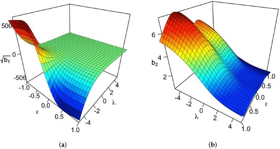
Figure 2. (a) Asymmetry coefficient and (b) kurtosis coefficient for btpn$(\sigma =1,\lambda ,ϵ)$ distribution.

2.3. Mode and Unimodality and Bimodality Regions

The next proposition presents the unimodality and bimodality property of the btpn distribution.

Proposition 6.

Let $X\sim btpn(\sigma ,\lambda ,ϵ)$. For $\lambda \le 0$, the model is unimodal, and for $\lambda >0$, the model is bimodal. Moreover, for the unimodal case, the mode of the model is 0, and for the bimodal case, the two modes are $-\sigma \lambda (1+ϵ)$ and $\sigma \lambda (1-ϵ)$, respectively.

Proof. 

By definition, the mode is the value that maximizes the pdf or, equivalently, the logarithm of the pdf. For $X\sim btpn(\sigma ,\lambda ,ϵ)$, it is straighforward to show that

$$\begin{array}{cc}\hfill \frac{\partial \log f(x;\sigma ,\lambda ,ϵ)}{\partial x}& =\{\begin{array}{cc}-\frac{1}{\sigma (1+ϵ)}\left(\frac{x}{\sigma (1+ϵ)}+\lambda \right)\hfill & ,\mathrm{if} x<0\hfill \\ -\frac{1}{\sigma (1-ϵ)}\left(\frac{x}{\sigma (1-ϵ)}-\lambda \right)\hfill & ,\mathrm{if} x\ge 0\hfill \end{array} \mathrm{and}\hfill \\ \hfill \frac{{\partial }^2\log f(x;\sigma ,\lambda ,ϵ)}{\partial x^2}& =\{\begin{array}{cc}-\frac{1}{{\sigma }^2{(1+ϵ)}^2}\hfill & ,\mathrm{if} x<0\hfill \\ -\frac{1}{{\sigma }^2{(1-ϵ)}^2}\hfill & ,\mathrm{if} x\ge 0\hfill \end{array}.\hfill \end{array}$$

Therefore, solving the equation $\partial \log f(x;\sigma ,\lambda ,ϵ)/\partial x=0$, we obtain $x_1=-\sigma \lambda (1+ϵ)$ and $x_2=\sigma \lambda (1-ϵ)$ as the potential mode for each branch, because the second derivative is negative for each respective case. However, this is valid if and only if $x_1<0$ and $x_2>0$, respectively. In other words, if $-\sigma \lambda (1+ϵ)<0$, then $x_1$ is a mode and if $\sigma \lambda (1-ϵ)>0$, then $x_2$ also is a mode. This is equivalent to

$$\begin{array}{cc}\hfill \{\lambda >0\wedge 1+ϵ>0\}& \vee \{\lambda <0\wedge 1+ϵ<0\}\Rightarrow x_1 \mathrm{is} \mathrm{a} \mathrm{mode} \mathrm{and}\hfill \\ \hfill \{\lambda >0\wedge 1-ϵ>0\}& \vee \{\lambda <0\wedge 1-ϵ<0\}\Rightarrow x_2 \mathrm{is} \mathrm{a} \mathrm{mode}.\hfill \end{array}$$

where $1+ϵ>0$ and $1-ϵ>0$, $\forall ϵ(-1,1)$. On the other hand, $1+ϵ\nless 0$ and $1-ϵ\nless 0$. For this reason, it is immediate that for $\lambda >0$, the btpn distribution have two modes, and such modes are $x_1$ and $x_2$. Finally, for $\lambda \le 0$, it is immediate that $\partial \log f(x;\sigma ,\lambda ,ϵ)/\partial x>0$, for $x<0$ and $\partial \log f(x;\sigma ,\lambda ,ϵ)/\partial x\le 0$ for $x\ge 0$. In other words, the pdf for the btpn distribution is an increasing function in $(-\infty ,0)$ and a decreasing function in $(0,\infty )$, where we can deduce that the model is unimodal and the respective mode is attached in zero. □

Figure 3 shows the regions of unimodality and bimodality for the btpn depending on the parameters $\lambda$ and $ϵ$.

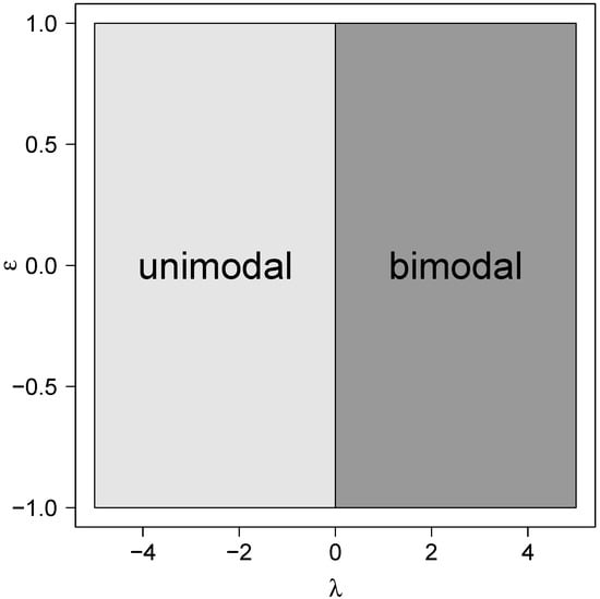
Figure 3. Regions of unimodality and bimodality for the btpn model in terms of $\lambda$ and $\eta$.

2.4. Particular Cases

By construction, the following models are particular cases for the btpn distribution:

• btpn$(\sigma =\sigma /2,\lambda ,ϵ=-1)\equiv$ tpn$(\sigma ,\lambda )$;
• btpn$(\sigma ,\lambda =0,ϵ=0)\equiv$ N$(0,{\sigma }^2)$, i.e., the normal distribution with mean 0 and variance ${\sigma }^2$;
• btpn$(\sigma =1,\lambda =0,ϵ)\equiv$ esn$(\sigma ,ϵ)$, i.e., the epsilon skew-normal distribution (Mudholkar and Hutson [10]).

Figure 4 summarizes the relationships among the btpn and its particular cases.

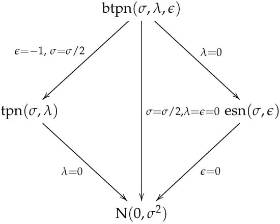
Figure 4. Particular cases for the btpn distribution.

3. Inference

In this section, we discuss the maximum likelihood (ML) method for parameter estimation for the btpn model. We also provide details about the computational aspects.

3.1. Maximum Likelihood Function

Hereafter, and to simplify the estimation procedure, we consider the reparameterization $\eta =\frac{ϵ}{\sqrt{1-{ϵ}^2}}\in \mathbb{R}$. Therefore, henceforth, we denote $X\sim btpn(\sigma ,\lambda ,\eta )$, with $\sigma$, $\lambda$ and $\eta$ scale, shape and asymmetry parameters, respectively, if its pdf is given by

$$f(x;\sigma ,\lambda ,\eta )=\{\begin{array}{cc}\frac{1}{2\sigma \mathsf{\Phi }\left(\lambda \right)}\varphi \left(\frac{-x\sqrt{1+{\eta }^2}}{\sigma (\sqrt{1+{\eta }^2}+\eta )}-\lambda \right)\hfill & ,\mathrm{if} x<0\\ \frac{1}{2\sigma \mathsf{\Phi }\left(\lambda \right)}\varphi \left(\frac{x\sqrt{1+{\eta }^2}}{\sigma (\sqrt{1+{\eta }^2}-\eta )}-\lambda \right)\hfill & ,\mathrm{if} x\ge 0\end{array}$$

Given $z_1,\dots ,z_n$, a random sample from the btpn$(\sigma ,\lambda ,\eta )$ distribution, the log-likelihood function for $\mathit{\theta }=(\sigma ,\lambda ,\eta )$ is given by

$$\ell \left(\mathit{\theta }\right)=-n\left[\log \left(2\sigma \mathsf{\Phi }\left(\lambda \right)\right)+\frac{1}{2}\log \left(2\pi \right)+\frac{{\lambda }^2}{2}\right]+{\ell }_1\left(\mathit{\theta }\right)+{\ell }_2\left(\mathit{\theta }\right),$$

(1)

where

$$\begin{array}{cc}\hfill {\ell }_1\left(\mathit{\theta }\right)& =-\frac{1}{2}\sum _{i:z_i\le 0}\left\{{\left(\frac{z_i\sqrt{1+{\eta }^2}}{\sigma (\sqrt{1+{\eta }^2}-\eta )}\right)}^2-\frac{2z_i\lambda \sqrt{1+{\eta }^2}}{\sigma (\sqrt{1+{\eta }^2}-\eta )}\right\}, \mathrm{and}\hfill \\ \hfill {\ell }_2\left(\mathit{\theta }\right)& =-\frac{1}{2}\sum _{i:z_i>0}\left\{{\left(\frac{z_i\sqrt{1+{\eta }^2}}{\sigma (\sqrt{1+{\eta }^2}+\eta )}\right)}^2+\frac{2z_i\lambda \sqrt{1+{\eta }^2}}{\sigma (\sqrt{1+{\eta }^2}+\eta )}\right\}.\hfill \end{array}$$

To find the ML estimator of $\mathit{\theta }$, say $\widehat{\mathit{\theta }}$, we need to maximize $\ell \left(\mathit{\theta }\right)$ in (1) in relation to $\mathit{\theta }$. However, no closed-form expressions for the ML estimates are possible. Therefore, we must use an iterative method for nonlinear optimization. For instance, we solve this problem using the Broyden-–Fletcher–-Goldfarb–-Shanno (BFGS) quasi-Newton method; see [11] (p. 199).

3.2. Computational Aspects

The ML estimators for the btpn model and the obtaining of their standard errors are included in the tpn package [12] from the R [13] software. The following function can be used to obtain these results:

•     est.btpn(y)

where y is the sample. The function returns a list with the estimates, the iterations used for the maximization algorithm, the log-likelihood function evaluated in the parameter estimations and the corresponding Akaike information criterion (AIC, see [14]) and the Bayesian information criterion (BIC, see [15]). Models with lower AIC and/or BIC are preferable. The package also includes the functions to drawn values to evaluate the pdf and the cdf for the btpn model named rbtpn, dbptn and pbtpn, respectively.

4. Simulation Study

In this section, we present a simulation study in order to evaluate the behaviour of the ML estimators in finite samples. The study was conducted using the tpn package [12]. Specifically, random samples were generated using the rbtpn function, and the estimation was performed using the est.btpn function. We considered 5000 Monte Carlo replicates for 3 sample sizes: 50, 100 and 200. We also considered 2 combinations for the scale parameter $\sigma$: 2 and 10; 3 values for $\lambda$: $-0.75,1$ and 3; and 2 values for $\eta$: $-0.5$ and $0.75$. This setting provides 36 combinations of the parameters $\sigma ,\lambda$ and $\eta$ and the sample size. Table 1 and Table 2 summarize the empirical bias, the standard errors of the MLE (SE), the root-mean-squared error (RMSE) and the 95% coverage probability (CP) based on the asymptotic distribution of the MLE. In general terms, the bias and RMSE terms are reduced when the sample size is increased, suggesting the consistency of the MLE. Note also that the SE and RMSE terms are closer when the sample size is increased, suggesting that the standard errors of the estimators are also well estimated. Additionally, the CP terms converge reasonably to the nominal value used to their construction (95%), suggesting that the normality is reasonable as an asymptotic distribution to the ML estimators in the btpn model, even in reasonable sample sizes.

Table 1. Empirical bias, SE, RMSE and 95% CP for the ML estimators of $\sigma ,\lambda$ and $\eta$ in the btpn distribution with different combinations of parameters (case true $\sigma =2$).

True Value			$\mathit{n}=50$				$\mathit{n}=100$				$\mathit{n}=200$
$\mathit{\lambda }$	$\mathit{\eta }$	par.	bias	SE	RMSE	CP	bias	SE	RMSE	CP	bias	SE	RMSE	CP
−0.75	−0.5	$\sigma$	0.894	3.271	8.403	0.814	0.170	1.089	3.165	0.856	0.035	0.514	0.584	0.898
		$\lambda$	−0.831	3.405	8.561	0.862	−0.132	1.237	3.050	0.891	−0.028	0.638	0.691	0.917
		$\eta$	−0.018	0.112	0.121	0.940	−0.008	0.078	0.081	0.945	−0.003	0.055	0.057	0.947
	0.75	$\sigma$	0.736	2.490	7.381	0.802	0.233	1.218	3.497	0.862	0.041	0.538	0.630	0.901
		$\lambda$	−0.663	2.663	7.325	0.855	−0.205	1.368	3.453	0.897	−0.029	0.660	0.728	0.924
		$\eta$	0.030	0.142	0.167	0.936	0.014	0.099	0.106	0.945	0.009	0.070	0.073	0.947
1	−0.5	$\sigma$	−0.057	0.350	0.360	0.887	−0.026	0.248	0.250	0.914	−0.012	0.175	0.176	0.936
		$\lambda$	0.073	0.406	0.416	0.938	0.035	0.285	0.289	0.946	0.014	0.201	0.201	0.949
		$\eta$	−0.014	0.086	0.095	0.932	−0.008	0.061	0.064	0.940	−0.003	0.043	0.045	0.944
	0.75	$\sigma$	−0.055	0.350	0.355	0.884	−0.024	0.248	0.251	0.919	−0.015	0.174	0.176	0.931
		$\lambda$	0.072	0.406	0.412	0.935	0.035	0.285	0.288	0.943	0.020	0.200	0.203	0.942
		$\eta$	0.028	0.109	0.127	0.940	0.012	0.076	0.082	0.942	0.006	0.054	0.055	0.943
3	−0.5	$\sigma$	−0.049	0.203	0.214	0.919	−0.022	0.145	0.152	0.930	−0.013	0.103	0.106	0.936
		$\lambda$	0.103	0.356	0.383	0.948	0.047	0.248	0.262	0.947	0.028	0.174	0.180	0.948
		$\eta$	−0.007	0.051	0.054	0.937	−0.003	0.036	0.036	0.949	−0.001	0.025	0.026	0.950
	0.75	$\sigma$	−0.048	0.203	0.214	0.917	−0.023	0.145	0.148	0.932	−0.012	0.103	0.103	0.946
		$\lambda$	0.105	0.356	0.385	0.946	0.046	0.248	0.253	0.952	0.024	0.174	0.175	0.953
		$\eta$	0.011	0.064	0.072	0.933	0.005	0.045	0.048	0.939	0.002	0.032	0.033	0.942

Table 2. Empirical bias, SE, RMSE and 95% CP for the ML estimators of $\sigma ,\lambda$ and $\eta$ in the btpn distribution with different combinations of parameters (case true $\sigma =10$).

True Value			$\mathit{n}=50$				$\mathit{n}=100$				$\mathit{n}=200$
$\mathit{\lambda }$	$\mathit{\eta }$	par.	bias	SE	RMSE	CP	bias	SE	RMSE	CP	bias	SE	RMSE	CP
−0.75	−0.5	$\sigma$	2.279	10.597	19.571	0.802	0.961	5.254	11.695	0.864	0.221	2.538	3.411	0.900
		$\lambda$	−0.400	2.336	4.023	0.857	−0.161	1.209	2.328	0.896	−0.034	0.632	0.780	0.924
		$\eta$	−0.020	0.112	0.126	0.938	−0.009	0.079	0.083	0.949	−0.004	0.055	0.056	0.950
	0.75	$\sigma$	1.748	9.147	17.694	0.797	0.608	5.063	7.312	0.859	0.157	2.496	3.225	0.891
		$\lambda$	−0.272	2.046	3.498	0.856	−0.093	1.172	1.548	0.895	−0.021	0.623	0.734	0.920
		$\eta$	0.038	0.143	0.177	0.933	0.013	0.099	0.103	0.951	0.007	0.069	0.072	0.945
1	−0.5	$\sigma$	−0.225	1.772	1.829	0.887	−0.126	1.237	1.260	0.916	−0.057	0.876	0.891	0.932
		$\lambda$	0.065	0.408	0.415	0.938	0.037	0.285	0.289	0.940	0.015	0.201	0.205	0.943
		$\eta$	−0.014	0.086	0.095	0.936	−0.005	0.060	0.063	0.943	−0.002	0.043	0.043	0.952
	0.75	$\sigma$	−0.284	1.744	1.756	0.886	−0.136	1.236	1.255	0.913	−0.059	0.875	0.869	0.933
		$\lambda$	0.073	0.405	0.405	0.941	0.037	0.285	0.288	0.943	0.016	0.201	0.201	0.946
		$\eta$	0.028	0.109	0.131	0.926	0.012	0.076	0.081	0.945	0.008	0.054	0.056	0.946
3	−0.5	$\sigma$	1.985	2.784	30.165	0.913	1.699	1.824	26.982	0.928	1.113	0.799	22.887	0.932
		$\lambda$	0.023	0.420	1.320	0.941	−0.032	0.287	1.178	0.947	−0.025	0.184	0.955	0.941
		$\eta$	−0.004	0.051	0.054	0.934	−0.002	0.036	0.037	0.944	−0.001	0.026	0.026	0.948
	0.75	$\sigma$	0.386	4.618	13.399	0.918	0.596	1.816	14.121	0.924	0.355	0.929	10.561	0.943
		$\lambda$	0.071	0.474	0.692	0.954	0.016	0.285	0.680	0.941	0.003	0.188	0.503	0.952
		$\eta$	0.019	0.065	0.076	0.925	0.015	0.046	0.051	0.935	0.008	0.033	0.034	0.941

5. Application

In this section, we present an application to a real data set in order to illustrate the btpn model. We consider the height data set, which consists of the height of 126 students from the University of Pennsylvania (Cruz-Medina [16]). We compare our proposal with other bimodal proposals, such as the epsilon skew inverted gamma (esig, see Abdulah et al. [17]) and the alpha skew-normal (asn, Elal-Olivero [18]). The pdf for the esig model is given by:

$$f(x;\sigma ,\lambda ,\eta )=\frac{{\lambda }^{\sigma }}{2\Gamma \left(\sigma \right)}\{\begin{array}{cc}{\left(\frac{x}{1-\eta }\right)}^{-(\sigma +1)}{e}^{-\frac{\lambda (1-\eta )}{x}}& x\ge 0\\ {\left(\frac{-x}{1+\eta }\right)}^{-(\sigma +1)}{e}^{-\frac{\lambda (1+\eta )}{-x}}& x<0\end{array},$$

where $\lambda >0$, $\sigma >0$ and $\left|\eta \right|<1$ are the scale, shape and skewness parameters, respectively.

The pdf for the asn model is given by:

$$f(x;\eta ,\lambda ,\sigma )=\left(\frac{{[1-\eta \left(\frac{x-\lambda }{\sigma }\right)]}^2+1}{\sigma (2+{\eta }^2)}\right)\varphi \left(\frac{x-\lambda }{\sigma }\right),$$

where $\eta ,\lambda \in \mathbb{R}$ and $\sigma >0$ are the shape, location and scale parameters, respectively.

Table 3 summarizes some descriptive statistics for the sample, where we highlight the symmetrical behaviour of the data ($\sqrt{b_1}=-0.05$).

Table 3. Descriptive statistics for the $height$ data set.

Data Set	n	$\overline{\mathit{X}}$	${\mathit{S}}^2$	$\sqrt{{\mathit{b}}_1}$	${\mathit{b}}_2$
weight measured	126	0	1	$-0.05$	$3.053$

Table 4 presents the estimatives, standard errors, AIC and BIC criteria for the mentioned models. Note that, based on both criteria, btpn presents a better fit than the rest of the distributions. Figure 5 shows the histogram for the height data and the pdf for the three considered distributions, where the better performance for the btpn in this data set is demonstrated. Moreover, as discussed in Proposition 6, $\widehat{\lambda }=0.496>0$ implies a bimodal model, and such modes are equal to $x_1=-0.402$ and $x_2=0.404$. In addition, the distribution of height is very close to symmetry.

Table 4. Estimated parameters and their standard errors (in parentheses) for the btpn, esig and asn models for the $height$ data set. The AIC and BIC criteria are also presented.

Estimated	btpn	esig	asn
$\sigma$	0.813 (0.113)	1.304 (0.148)	0.996 (0.063)
$\lambda$	0.496 (0.316)	0.527 (0.073)	0.014 (3.422)
$\eta$	−0.002 (0.048)	0.095 (0.059)	0.014 (3.409)
AIC	360.76	415.79	362.67
BIC	369.27	424.30	375.91

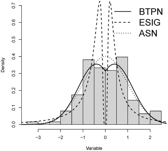
Figure 5. Histogram for the $height$ data set and the estimated pdf for the btpn, esig and asn models.

We also compute the randomized quantile residuals [19] for the three fitted models. If the model was correctly specified, these residuals should be a random sample from the standard normal distribution. Figure 6 shows the qqplot for such residuals, also suggesting that the btpn is a more appropriated model for this data set.

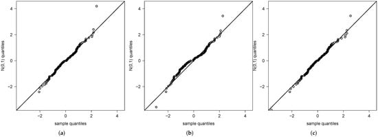
Figure 6. Quantile residuals for fitted models: (a) asn, (b) esig, and (c) btpn.

6. Conclusions

The importance of fitting an observable dataset by a probability distribution is well-known, since it will be covered with convenient properties. Difficulty arises when the data is bimodal, because there are not traditional distributions with this property. This gap is being filled by an increasing movement in the statistical literature to develop probability distributions which already have a bimodality feature. In this paper, we made our contribution with the bimodal positive truncation normal distribution. The btpn distribution has the following advantages: support in the real line, closed-form cdf and moments, and the ability to generalize the standard normal and treatable maximum likelihood estimators. The ML procedure works very reasonably, i.e, as the sample size increases, the bias and the SE decrease. Since there are models for which the estimation procedure does not work even for large samples, the btpn distribution also has this strength. We ended the advantages of our proposed distribution with an application where btpn was the best choice of fitting. As suggestions for future work, we can mention two possibilities: the first entails the improvement of the asymptotic properties of the ML estimation through bias and variance corrections (see [20,21], respectively), and the second involves the addition of a regression structure. A closed-form cdf allows even a quantile regression structure, see [22,23], for instance, as [24] did for the gamma–sinh Cauchy distribution. For the applicability and possibilities of future works, we think the bimodal positive truncation normal distribution is useful for practitioners and researchers of many different areas.

References

- Ashman, K.M.; Bird, C.M.; Zepf, S.E. Detecting Bimodality in Astronomical Datasets. Astron. J. 1994, 108, 2348–2361. [Google Scholar] [CrossRef] [Green Version]
- Michele, C.; Accatino, F. Tree cover bimodality in savannas and forests emerging from the switching between two fire dynamics. PLoS ONE 2014, 9, e91195. [Google Scholar] [CrossRef] [PubMed] [Green Version]
- Wang, J.; Wen, S.; Symmans, W.F.; Pusztai, L.; Coombes, K.R. The bimodality index: A criterion for discovering and ranking bimodal signatures from cancer gene expression profiling data. Cancer Inform. 2009, 7, 199–216. [Google Scholar] [CrossRef] [PubMed] [Green Version]
- Robertson, C.A.; Fryer, J.G. Some descriptive properties of normal mixtures. Scand. Actuar. J. 1969, 3–4, 137–146. [Google Scholar] [CrossRef]
- Gómez, H.W.; Elal-Olivero, D.; Salinas, H.S.; Bolfarine, H. Bimodal extension based on the skew-normal distribution with application to pollen data. Environmetrics 2011, 22, 50–62. [Google Scholar] [CrossRef]
- Venegas, O.; Salinas, H.S.; Gallardo, D.I.; Bolfarine, H.; Gómez, H.W. Bimodality based on the generalized skew-normal distribution. J. Stat. Comput. Simul. 2018, 88, 156–181. [Google Scholar] [CrossRef]
- Butt, N.S.; Khalil, M.G. A New Bimodal Distribution for Modeling Asymmetric Bimodal Heavy-Tail Real Lifetime Data. Symmetry 2020, 12, 2058. [Google Scholar] [CrossRef]
- Gómez, Y.M.; Gómez-Déniz, E.; Venegas, O.; Gallardo, D.I.; Gómez, H.W. An Asymmetric Bimodal Distribution with Application to Quantile Regression. Symmetry 2019, 11, 899. [Google Scholar] [CrossRef] [Green Version]
- Gómez, H.J.; Olmos, N.M.; Varela, H.; Bolfarine, H. Inference for a truncated positive normal distribution. Appl. Math. J. Chin. Univ. 2018, 33, 163–176. [Google Scholar] [CrossRef]
- Mudholkar, G.S.; Hutson, A.D. The epsilon–skew–normal distribution for analyzing near-normal data. J. Stat. Plan. Inference 2000, 83, 291–309. [Google Scholar] [CrossRef]
- Mittelhammer, R.C.; Judge, G.G.; Miller, D.J. Econometric Foundations; Cambridge University Press: New York, NY, USA, 2000. [Google Scholar]
- Gallardo, D.I.; Gómez, H.J.; Gómez, Y.M. tpn: Truncated Positive Normal Model and Extensions. R Package Version 1.1. 2021. Available online: https://cran.r-project.org/web/packages/tpn/index.html (accessed on 25 January 2022).
- R Core Team. R: A Language and Environment for Statistical Computing; R Foundation for Statistical Computing: Vienna, Austria, 2022; Available online: https://www.R-project.org/ (accessed on 25 January 2022).
- Akaike, H. A new look at the statistical model identification. IEEE Trans. Autom. Control 1974, 19, 716–723. [Google Scholar] [CrossRef]
- Schwarz, G. Estimating the dimension of a model. Ann. Stat. 1978, 6, 461–464. [Google Scholar] [CrossRef]
- Cruz-Medina, I.R.; Olmos, N.M. Almost Nonparametric and Nonparametric Estimation in Mixture Model. Ph.D. Thesis, Pennsylvania State University, State College, PA, USA, 2001. [Google Scholar]
- Abdulah, E.K.; Elsalloukh, H. Bimodal Class based on the Inverted Symmetrized Gamma Distribution with Applications. J. Stat. Appl. Probab. 2014, 3, 1–7. [Google Scholar] [CrossRef]
- Elal-Olivero, D. Alpha-skew-normal distribution. Proyecciones 2010, 29, 224–240. [Google Scholar] [CrossRef] [Green Version]
- Dunn, P.K.; Smyth, G.K. Randomized quantile residuals. J. Comput. Graph. Stat. 1996, 5, 236–244. [Google Scholar]
- Magalhães, T.M.; Gómez, Y.M.; Gallardo, D.I.; Venegas, O. Bias reduction for the Marshall-Olkin extended family of distributions with application to an airplane’s air conditioning system and precipitation data. Symmetry 2020, 12, 851. [Google Scholar] [CrossRef]
- Magalhães, T.M.; Botter, D.A.; Sandoval, M.C. A general expression for second-order covariance matrices—An application to dispersion models. Braz. J. Probab. Stat. 2021, 35, 37–49. [Google Scholar] [CrossRef]
- Cade, B.S.; Noon, B.R. A gentle introduction to quantile regression for ecologists. Front. Ecol. Environ. 2003, 1, 412–420. [Google Scholar] [CrossRef]
- Alencar, A.P.; Santos, B.R. Association of pollution with quantiles and expectations of the hospitalization rate of elderly people by respiratory diseases in the city of São Paulo, Brazil. Environmetrics 2014, 25, 165–171. [Google Scholar] [CrossRef]
- Gómez, Y.M.; Gallardo, D.I.; Venegas, O.; Magalhães, T.M. An asymmetric bimodal double regression model. Symmetry 2021, 13, 2279. [Google Scholar] [CrossRef]
Publisher’s Note: MDPI stays neutral with regard to jurisdictional claims in published maps and institutional affiliations. |
© 2022 by the authors. Licensee MDPI, Basel, Switzerland. This article is an open access article distributed under the terms and conditions of the Creative Commons Attribution (CC BY) license (https://creativecommons.org/licenses/by/4.0/).