Numerical Investigation of the Two-Dimensional Fredholm Integral Equations of the Second Kind by Bernstein Operators

Abstract

In this study, the numerical solutions of linear two-dimensional Fredholm integral equations of the second kind via Bernstein operators are considered. The method is presented with illustrative examples for regularized-equal and Chebyshev collocation points. The obtained numerical results from illustrative examples show that the proposed numerical algorithm is accurate and efficient for solving linear two-dimensional Fredholm integral equation of the second kind.

1. Introduction

Let $D:=\left[0,1\right]\times [0,1]$. Two dimensional linear Fredholm integral equations of the second kind

$$\alpha (x,y)u(x,y)-\beta (x,y)\underset{0}{\overset{1}{\int }}\underset{0}{\overset{1}{\int }}\kappa (x,y;s,t)u(s,t)dsdt=f(x,y),(x,y)\in D$$

(1)

is considered, where $\alpha (x,y)$, $\beta (x,y)$ and $f(x,y)$ are given non-zero continuos functions on D. $\kappa (x,y;s,t)\in C(D\times D)$ (i.e., continuous space on $D\times D$) is the kernel function, and $u(x,y)$ is the undetermined function. Fredholm and Volterra integral equations often appear in science and engineering problems. For example Fredholm integral equations arise in mathematical economics (see [1]), in fluid mechanics problems involving hydrodynamic interactions near finite-sized elastic interfaces (see [2,3]) and in physics; for the mass distribution of polymers in a polymeric melt [4]. Volterra integral equations are important for initial value problems of differential equations (see [5]). See also [6,7,8] for more applications of Fredholm and Volterra integral equations in mathematical physics. Obtaining the analytical solutions of integral equations is difficult, so the numerical solutions of integral equations are necessary.

There are some numerical methods for solving integral equations of the second kind, such as the Bernstein piecewise polynomial method, integral mean value method, Taylor series method and least square method as presented in [9] for one dimensional Fredholm integral equations. A simple numerical method based on Berstein’s approximation for Volterra integral equation is presented in [10] for one dimension, and authors approximate unknown function by Bernstein’s polynomial approximation. Bivariate generalized Bernstein operators are used to solve Fredholm integral equations in [11] with applications. Lagrange polynomial approximation, Barycentric Lagrange polynomial approximation, and modified Lagrange polynomial approximation were also used for numerical solutions of Volterra and Fredholm integral equations in [12] for one dimension, and in [13] for two dimensions. Cosine-trigonometric basis functions are developed to solve two dimensional Fredholm integral equations of the second kind, with accurate solution by [14]. Weakly singular kernel using spectral collocation is another technique for solving Fredholm integral equations of the second kind [15]. Modified Berstein–Kantorovich operators were used for numerical solutions of the Fredholm and Volterra integral equations, see [16]. Two-dimensional Volterra–Fredholm integral equations of the second kind are solved by Berstein operators, based on approximating unknown function with Bernstein polynomials [17]. Two dimensional Bernstein polynomial approximation method for mixed Fredholm-Volterra integral equations is presented in [18] with operational matrix. The method has several advantages in reducing computational burden with good accuracy. Moreover, Bernstein operators are useful to find the approximate solutions of the integral equations, see also [19,20,21,22,23].

This paper presents a two dimensional Bernstein polynomial approximation method with regularized-equal collocation points and with Chebyshev collocation points to solve two dimensional linear Fredholm integral equation of the second kind.

The sections of the paper are organized as follows: In Section 2, the two dimensional Bernstein polynomial approximation method is considered with regularized equally-spaced and with Chebyshev collocation points. A numerical approach based on the method given by [24] is developed for solving Fredholm integral equations of the second kind. In Section 3, the method is applied on some examples from literature. These numerical examples illustrate the efficiency and applicability of the method. The interpretations of the obtained results are given in Section 4.

2. Bernstein Polynomial Approximation Method

2.1. Two-Dimensional Bernstein Polynomial Approximation Method

Two dimesional Bernstein polynomials of degree $m\times n$ on the square $D:=[0,1]\times$$[0,1]$ are

$$\begin{array}{ccc}\hfill b_{(k,m),(p,n)}(x,y)& =& \left(\genfrac{}{}{0pt}{}{m}{k}\right)\left(\genfrac{}{}{0pt}{}{n}{p}\right)x^k{(1-x)}^{m-k}{y}^j{(1-y)}^{n-p},(x,y)\in D,\hfill \\ \hfill k& =& 0,1,\dots ,m,p=0,1,\dots ,n\in \mathbb{N}.\hfill \end{array}$$

(2)

Then, the Bernstein approximation $B_{m,n}\left(f(x,y)\right)$ to a function $f(x,y):$$D\to \mathbb{R}$ is the polynomial

$$B_{m,n}\left(f(x,y)\right)=\sum _{k=0}^m\sum _{p=0}^{n}f\left(\frac{k}{m},\frac{p}{n}\right)b_{(k,m),(p,n)}(x,y).$$

(3)

See [25] for the properties of Bernstein polynomials on D and convergency for fractional integration and see [17] for the properties of Bernstein polynomials on D and convergency of this approximation method for Volterra–Fredholm integral equations.

2.2. Discretization of the Integral Equations by Bernstein’s Approximation

Consider the following integral equation,

$$\alpha (x,y)u(x,y)-\beta (x,y)\underset{0}{\overset{1}{\int }}\underset{0}{\overset{1}{\int }}\kappa (x,y;s,t)u(s,t)dsdt=f(x,y),(x,y)\in D,$$

(4)

where, $\alpha (x,y)$, $\beta (x,y)$ and $f(x,y)$ are non-zero continuous functions on D. $\kappa (x,y;s,t)\in C$$\left(D\times D\right)$ is the kernel function and $u(x,y)$ is the undetermined function. The two dimensional Bernstein’s approximation $B_{m,n}\left(u(x,y)\right)$ of the $m\times n$ degree are defined on D as,

$$B_{m,n}\left(u(x,y)\right)=\sum _{k=0}^m\sum _{p=0}^{n}u\left(\frac{k}{m},\frac{p}{n}\right)b_{(k,m),(p,n)}(x,y),$$

(5)

where,

$$\begin{array}{ccc}\hfill b_{(k,m),(p,n)}(x,y)& =& \left(\genfrac{}{}{0pt}{}{m}{k}\right)\left(\genfrac{}{}{0pt}{}{n}{p}\right)x^k{(1-x)}^{m-k}{y}^p{(1-y)}^{n-p},(x,y)\in D,\hfill \\ \hfill k& =& 0,1,\dots ,m,p=0,1,\dots ,n\in \mathbb{N}.\hfill \end{array}$$

(6)

In order to find $u(\frac{k}{m},\frac{p}{n})$, $k=0,1,\dots ,m,$$p=0,1,\dots ,n$ convert (4) into a linear form by using the collocation points $x_i$, $i=0,1,\dots ,m$, and $y_j$, $j=0,1,\dots ,n$ and approximating the unknown function $u(x,y)$ by (5). That is,

$$\begin{array}{ccc}& & \alpha (x_i,y_j)\sum _{k=0}^m\sum _{p=0}^{n}u(\frac{k}{m},\frac{p}{n})b_{(k,m),(p,n)}(x_i,y_j)\hfill \\ & & -\beta (x_i,y_j)\underset{0}{\overset{1}{\int }}\underset{0}{\overset{1}{\int }}\kappa (x_i,y_j;s,t)\sum _{k=0}^m\sum _{p=0}^{n}u(\frac{k}{m},\frac{p}{n})b_{(k,m),(p,n)}(s,t)dsdt\hfill \\ & =& f(x_i,y_j),(x_i,y_j)\in D.\hfill \end{array}$$

(7)

Choose collocation points $x_i$, $i=0,1,\dots ,m$ and $y_j$, $j=0,1,\dots ,n$ as regularized-equally spaced

$$x_i=\left\{\begin{array}{c}\epsilon +\frac{i}{m},\mathrm{for}i\ne m\\ 1-\epsilon ,\mathrm{for}i=m\end{array}\right.\mathrm{and}{y}_j=\left\{\begin{array}{c}\epsilon +\frac{j}{n},\mathrm{for}j\ne n\\ 1-\epsilon ,\mathrm{for}j=n\end{array}\right.$$

(8)

for arbitrary small $\epsilon$ to get rid of the undetermined computations as $0^0$ in the Equation (7) [10]. On the other hand, in the practical calculation, the second Chebyshev collocation points $(x_i,y_j),$ $i=0,1,\dots ,m$, $j=0,1,\dots ,n$ are takenas;

$$x_i=\left\{\begin{array}{c}\frac{1-cos\frac{i\pi }{m}}{2}+\epsilon ,\mathrm{for}i\ne m,i\ne 0\\ 1-\epsilon ,\mathrm{for}i=m\end{array}\right.\mathrm{and}{y}_j=\left\{\begin{array}{c}\frac{1-cos\frac{j\pi }{n}}{2}+\epsilon ,\mathrm{for}j\ne n,j\ne 0\\ 1-\epsilon ,\mathrm{for}j=n\end{array}\right..$$

(9)

Equivalently, (7) can be written in the matrix form

$$AX=Y,$$

(10)

where, the coefficient matrix $A\in {\mathbb{R}}^{(m+1)(n+1)\times (m+1)(n+1)}$ is

$$\begin{array}{ccc}\hfill A& =& \left[\alpha (x_i,y_j)b_{(k,m),(p,n)}(x_i,y_j)-\beta (x_i,y_j)\underset{0}{\overset{1}{\int }}\underset{0}{\overset{1}{\int }}\kappa (x_i,y_j;s,t)b_{(k,m),(p,n)}(s,t)dsdt\right]\hfill \\ \hfill i& =& 0,1,\dots ,m,j=0,1,\dots ,n,k=0,1,\dots ,m,p=0,1,\dots ,n,\hfill \end{array}$$

(11)

right side vector is

$$Y={\left[f(x_i,y_j)\right]}^T,i=0,1,\dots ,m,j=0,1,\dots ,n,$$

and the unknown vector X given as

$$X={\left[u_{m,n}(\frac{k}{m},\frac{p}{n})\right]}^T.$$

Algorithm 1: Numerical solution of the two dimensional Fredholm integral equation of the second kind by using Bernstein polynomial approximation $B_{m,n}\left(u(x,y)\right)$, is obtained as follows:

STEP 1. Put the m and n values. STEP 2. Set the collocation points $x_i$, $i=0,1,\dots ,m$ and $y_j$, $j=0,1,\dots ,n$, as in (8) or (9). STEP 3. Use STEP 1 and STEP 2 by Equation (11) to find matrix A. STEP 4. Calculate $Y={\left[f(x_i,y_j)\right]}^T$, $i=0,1,\dots ,m,$ $j=0,1,\dots ,n$. STEP 5. Solve the system (10) and denote the numerical solution by $u_{m,n}(\frac{k}{m},\frac{p}{n})$. STEP 6. Substitute $u_{m,n}(\frac{k}{m},\frac{p}{n})$ in Equation (5) and compute $B_{m,n}\left(u_{m,n}(\frac{k}{m},\frac{p}{n})\right)$. STEP 7. Calculate the error function $E(x,y)=$$u(x,y)-B_{m,n}\left(u_{m,n}(x,y)\right)$.

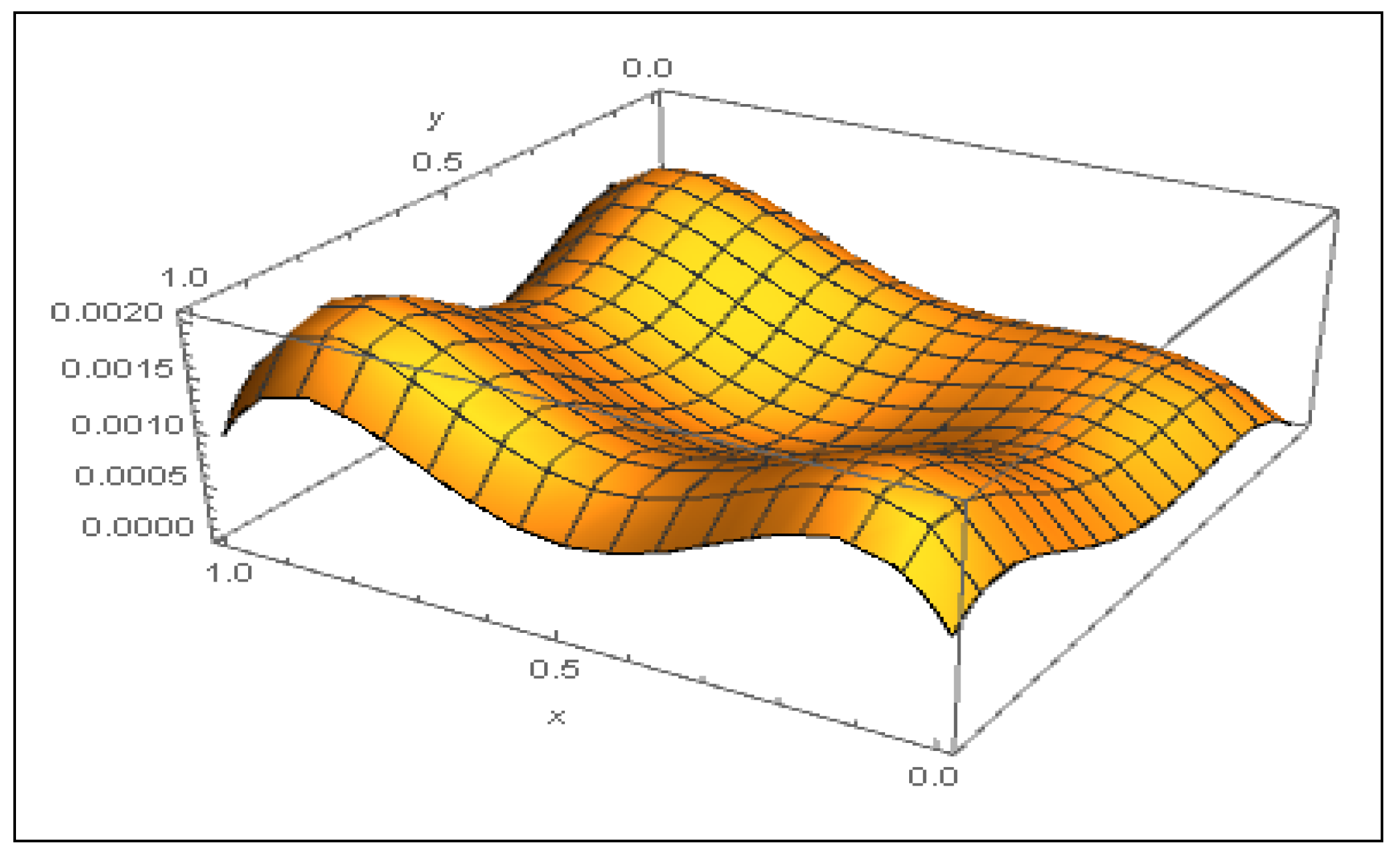
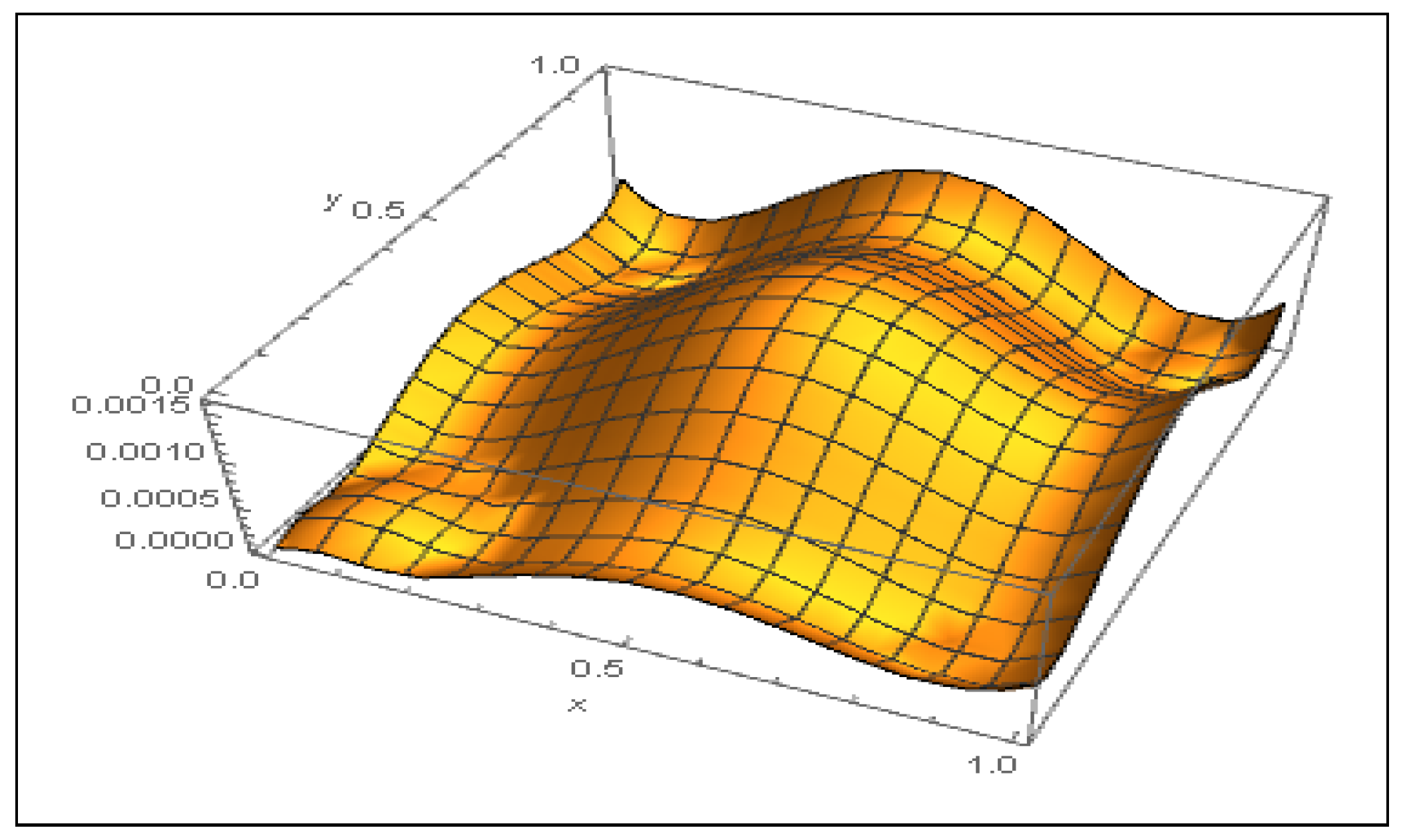
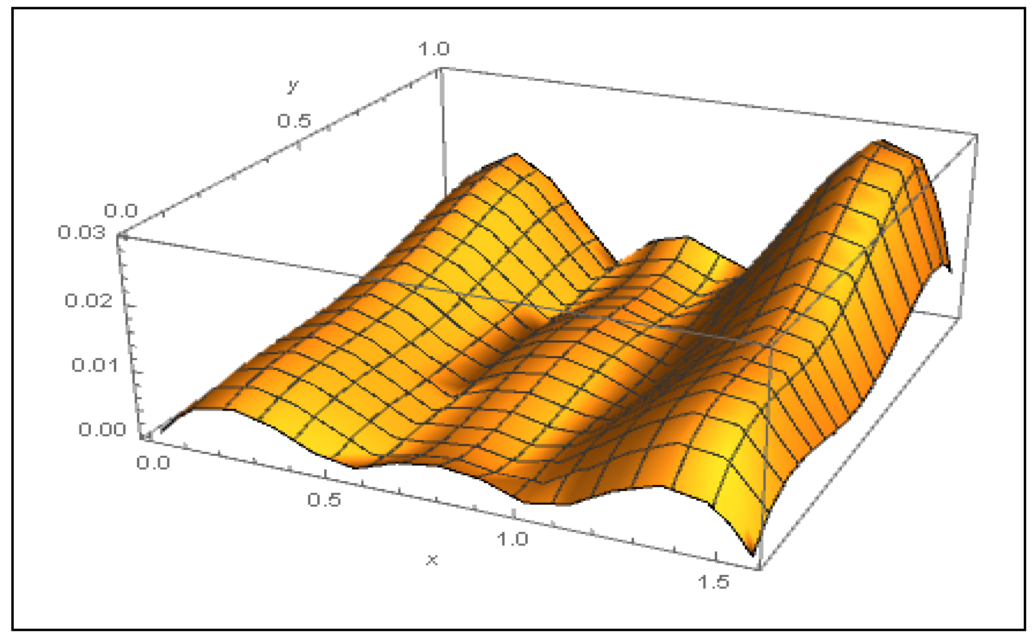
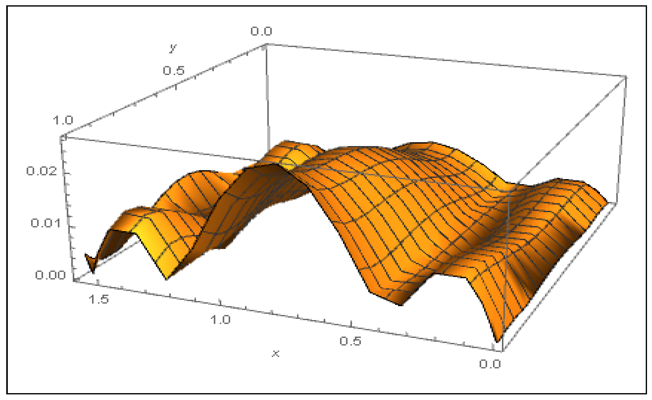
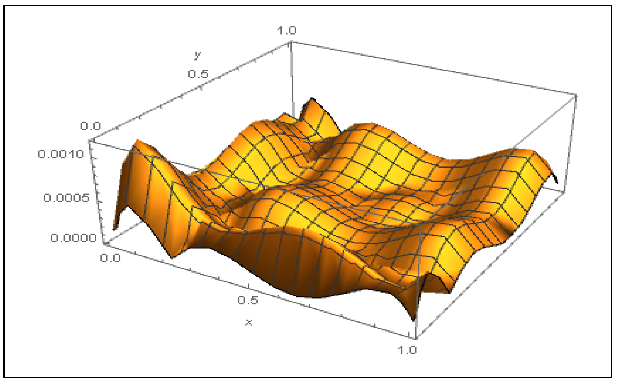
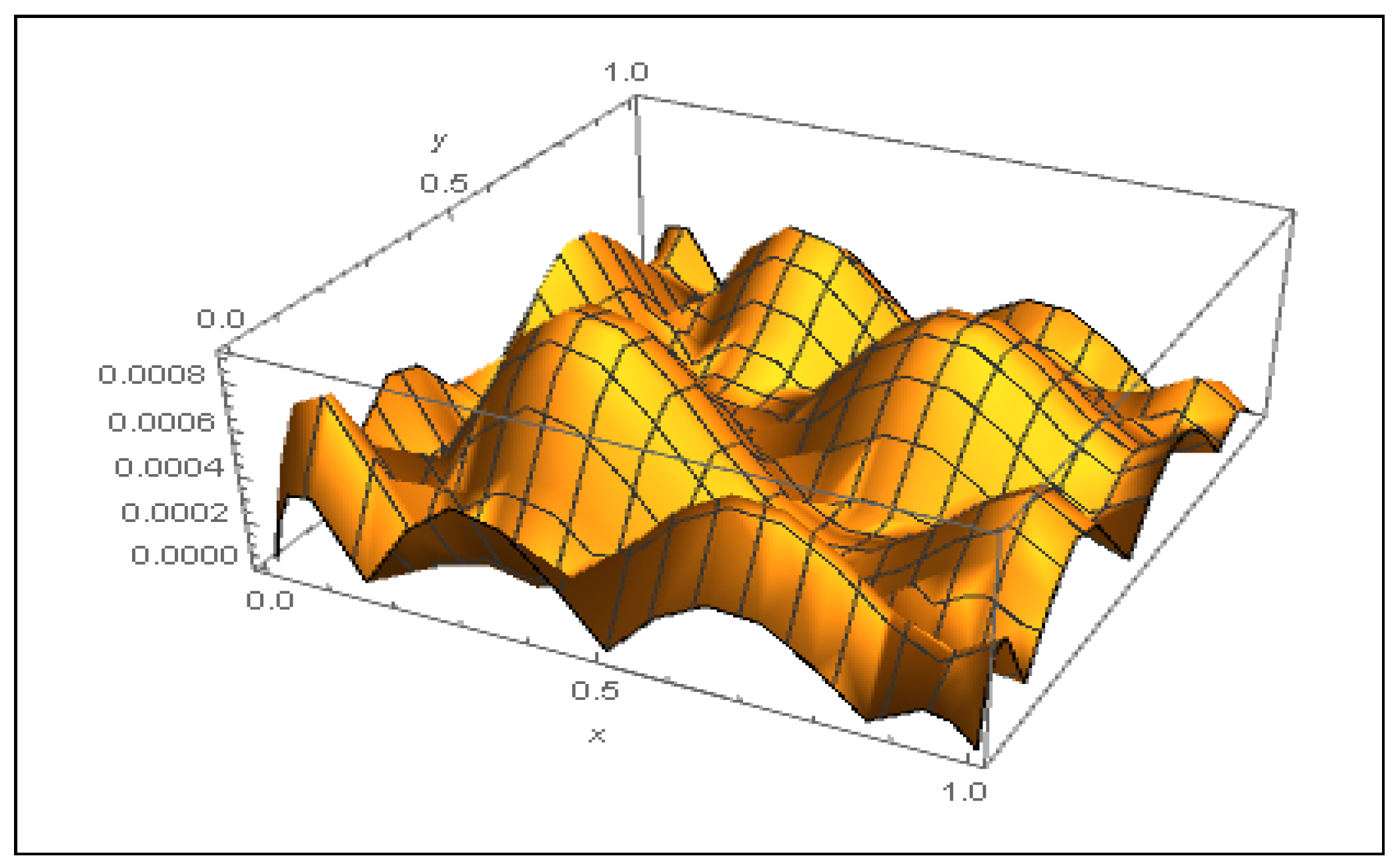
3. Numerical Results

In this numerical section, three test problems are used with the following errors. Let $x_p,$$p=0,1,\dots ,N_1$ and $y_q,$$q=0,1,\dots ,N_2$ be the selected points, where $N_1$ and $N_2$ are not necessarily equal to m and n, respectively. i.e., Error can be calculated for different number of selected points We define maximum and root mean square errors by

$$E(x,y)=u(x,y)-B_{m,n}\left(u_{m,n}(x,y)\right)$$

(12)

$$e_{p,q}=E(x_p,y_q)$$

(13)

$$e=\underset{p,q}{max}\left|e_{p,q}\right|$$

(14)

$$RMSE=\sqrt{\frac{1}{(N_1+1)(N_2+1)}\sum _{q=0}^{N_2}\sum _{p=0}^{N_1}{e}_{p,q}^2}$$

(15)

respectively. We use the notation $cond\left(A\right)$ to present the condition number of matrix A. Mathematica in double precision is used, to solve the examples. The exact solutions are known and used to show that the numerical solutions obtained by Bernstein polynomial approximation is correct. Moreover, “GaussKronrodRule” is used for numerical integration.

Example 1.

Let $D:=[0,1]\times [0,1]$. We consider the integral equation,

$$u(x,y)=sin(x+y)\underset{0}{\overset{1}{\int }}\underset{0}{\overset{1}{\int }}u(s,t)dtds+f(x,y),(x,y)\in D,$$

(16)

where $f(x,y)=[1+sin(2)-2sin(1\left)\right]sin(x+y)$, has the exact solution $u(x,y)=sin(x+y)$ [13]. The

Table 1. RMSE, maximum errors and $cond\left(A\right)$ obtained by Bernstein polynomial approximation with regularized-equal collocation points for the Example 1.

	RMSE	e	$\mathit{cond}\left(\mathit{A}\right)$
$m=4,n=4$	$8.38179\times {10}^{-4}$	$1.06334\times {10}^{-3}$	$57.8964$
$m=6,n=6$	$1.58843\times {10}^{-6}$	$2.00316\times {10}^{-6}$	$2094.98$
$m=8,n=8$	$2.12976\times {10}^{-9}$	$2.67504\times {10}^{-9}$	$\mathrm{83,023.7}$
$m=10,n=10$	$2.03771\times {10}^{-12}$	$2.55296\times {10}^{-12}$	$3.51706\times {10}^6$
$m=12,n=12$	$6.94695\times {10}^{-15}$	$9.21485\times {10}^{-15}$	$1.57479\times {10}^8$

presents the errors and $cond\left(A\right)$ in (11) of the linear system (10) by the given algorithm for regularized-equal collocation points in (8). The

Table 2. RMSE, maximum errors and $cond\left(A\right)$ obtained by Bernstein polynomial approximation with Chebyshev collocation points for the Example 1.

	RMSE	e	$\mathit{cond}\left(\mathit{A}\right)$
$m=4,n=4$	$4.83519\times {10}^{-4}$	$6.20168\times {10}^{-4}$	$45.0771$
$m=6,n=6$	$1.47242\times {10}^{-7}$	$1.88455\times {10}^{-7}$	$825.869$
$m=8,n=8$	$5.78929\times {10}^{-11}$	$7.39292\times {10}^{-11}$	$\mathrm{14,001.9}$
$m=10,n=10$	$2.49619\times {10}^{-14}$	$3.25295\times {10}^{-14}$	231,568
$m=12,n=12$	$5.89465\times {10}^{-15}$	$7.77156\times {10}^{-15}$	$3.82524\times {10}^6$

presents the errors and $cond\left(A\right)$ in (11) of the linear system (10) by the given algorithm for Chebyshev collocation points in (9).

The values of the approximate solution $u_{m,n}(x_i,y_j)$ at Chebyshev collocation points (9) are more accurate than at regularized equal collocation points. Usually, accuracy of the method is higher by Chebyshev collocation points than regularized equi-spaced points. Analogous results when Lagrange and Brycentric Lagrange methods were used to approximate the solution of two dimensional Fredholm integral equation of the second kind were also obtained in [13].

The $cond\left(A\right)$ of the coefficient matrix in (11) for Example 1 is increasing when the values m and n are increasing. This leads to ill-conditioning of the coefficient matrix A. Preconditioning techniques can be used for reducing the condition numbers see [26,27,28,29]. For example, a particular class of regular splittings of symmetric M-matrices was used to precondition the conjugate gradient (CG) method in [29]. Errors $\left|e_{p,q}\right|$ of Berstein polynomial approximation method for regularized-equal collocation points and for Chebyshev collocation points when $n=4$ and $m=4$ can be seen in Figure 1 and Figure 2, respectively.

Example 2.

Let $D_2:=[0,\pi /2]\times [0,1]$. Consider the following integral equation of the form

$$e^{x+y}u(x,y)=x^{2}y\underset{0}{\overset{\pi /2}{\int }}\underset{0}{\overset{1}{\int }}(x+y+s+t)u(s,t)dtds+f(x,y),(x,y)\in D_2,$$

(17)

where,

$$f(x,y)=(e-1)(1-e^{\pi /2})(x^{3}y+x^2{y}^2)+\left[(e-1)\left(e^{\pi /2}-\frac{e^{\pi /2}}{2}\pi -1\right)+(1-e^{\pi /2})\right]x^{2}y+e^{2x+2y},$$

and the exact solution is $u(x,y)=e^{x+y}$ [13].

Remark 1.

Regularized equally- spaced collocation points $x_i$, $i=0,1,\dots ,m$ and $y_j$, $j=0,1,\dots ,n$ for Example 2 are taken as

$$x_i=\left\{\begin{array}{c}\epsilon +\frac{\pi i}{2m},fori\ne m\\ \frac{\pi }{2}-\epsilon ,fori=m\end{array}\right.and{y}_j=\left\{\begin{array}{c}\epsilon +\frac{j}{n},forj\ne n\\ 1-\epsilon ,forj=n\end{array}\right.,$$

(18)

and Chebyshev collocation points are taken as,

$$x_i=\left\{\begin{array}{c}\frac{1}{2}(\frac{\pi }{2}-\frac{\pi }{2}cos\frac{i\pi }{m})+\epsilon ,fori\ne m,i\ne 0\\ \frac{\pi }{2}-\epsilon ,fori=m\end{array}\right.and{y}_j=\left\{\begin{array}{c}\frac{1-cos\frac{j\pi }{n}}{2}+\epsilon ,forj\ne n,j\ne 0\\ 1-\epsilon ,forj=n\end{array}\right..$$

(19)

The

Table 3. RMSE, maximum errors and $cond\left(A\right)$ matrix obtained by Bernstein polynomial approximation with regularized-equal collocation points for the Example 2.

	RMSE	e	$\mathit{cond}\left(\mathit{A}\right)$
$m=4,n=4$	$3.5208\times {10}^{-3}$	$8.13074\times {10}^{-3}$	$319.544$
$m=8,n=8$	$4.33182\times {10}^{-8}$	$1.05168\times {10}^{-7}$	370,059
$m=10,n=10$	$9.91076\times {10}^{-11}$	$2.42851\times {10}^{-10}$	$1.52628\times {10}^7$
$m=12,n=12$	$1.7907\times {10}^{-13}$	$4.3876\times {10}^{-13}$	$6.67461\times {10}^8$
$m=15,n=15$	$5.44544\times {10}^{-14}$	$1.35003\times {10}^{-13}$	$2.14727\times {10}^{11}$

presents the errors and $cond\left(A\right)$ of (11) for Example 2 with the given method for regularized-equal collocation points in (8). The

Table 4. RMSE, maximum errors and $cond\left(A\right)$ matrix obtained by Bernstein polynomial approximation with Chebyshev collocation points for the Example 2.

	RMSE	e	$\mathit{cond}\left(\mathit{A}\right)$
$m=4,n=4$	$1.92655\times {10}^{-3}$	$4.33359\times {10}^{-3}$	$313.093$
$m=8,n=8$	$1.24258\times {10}^{-9}$	$2.85366\times {10}^{-9}$	$\mathrm{81,233.1}$
$m=10,n=10$	$9.61004\times {10}^{-13}$	$2.21334\times {10}^{-12}$	$1.30198\times {10}^6$
$m=12,n=12$	$7.95505\times {10}^{-15}$	$2.66454\times {10}^{-14}$	$2.08914\times {10}^7$
$m=15,n=15$	$8.71513\times {10}^{-15}$	$2.4869\times {10}^{-14}$	$1.33228\times {10}^9$

presents the errors and $cond\left(A\right)$ of (11) for Example 2 with the given method for Chebyshev collocation points in (9).

Usually, solving the integral Equation (17) by Bernstein polynomial approximation with Chebyshev collocation points in (9) give more accurate solutions than with regularized-equal collocation points. $cond\left(A\right)$ of (10) is increasing according to m and n values. For this example ill-conditioned matrix is obtained when the m and n values are increased. Errors $\left|e_{p,q}\right|$ of Berstein polynomial approximation method for regularized-equal collocation points and for Chebyshev collocation points when $n=4$ and $m=4$ can be seen in Figure 3 and Figure 4, respectively.

Example 3.

Let $D:=[0,1]\times [0,1]$. We consider the following integral equation of the form

$$u(x,y)=\underset{0}{\overset{1}{\int }}\underset{0}{\overset{1}{\int }}(e^{x+y}+s+t)u(s,t)dtds+f(x,y),(x,y)\in D,$$

(20)

where, $f(x,y)=-\frac{46}{63}-\frac{4e^{x+y}}{7}+x^{5/2}+y^{5/2},$ has the exact solution $u(x,y)=x^{5/2}+y^{5/2}.$ The

Table 5. RMSE, maximum errors and $cond\left(A\right)$ obtained by Bernstein polynomial approximation with regularized equal collocation points for the Example 3.

	RMSE	e	$\mathit{cond}\left(\mathit{A}\right)$
$m=4,n=4$	$1.53888\times {10}^{-3}$	$2.67654\times {10}^{-3}$	$31.4408$
$m=8,n=8$	$1.34335\times {10}^{-5}$	$2.23442\times {10}^{-5}$	405,765
$m=10,n=10$	$3.77166\times {10}^{-6}$	$6.17914\times {10}^{-6}$	$1.73458\times {10}^7$
$m=12,n=12$	$1.40399\times {10}^{-6}$	$2.27531\times {10}^{-6}$	$7.74265\times {10}^8$
$m=13,n=13$	$7.40942\times {10}^{-7}$	$1.09405\times {10}^{-6}$	$5.5125\times {10}^9$
$m=14,n=14$	$6.25117\times {10}^{-7}$	$1.00499\times {10}^{-6}$	$3.56596\times {10}^{10}$
$m=15,n=15$	$3.67724\times {10}^{-7}$	$5.48086\times {10}^{-7}$	$2.54559\times {10}^{11}$

presents the errors and $cond\left(A\right)$ of (11) of the linear system (10) of Example 3 with the Bernstein polynomial approximation method for regularized-equal collocation points. The errors and $cond\left(A\right)$ of (11) of the linear system of Example 3 by the Bernstein polynomial approximation method with Chebyshev collocation points (9) are given in

Table 6. RMSE, maximum errors and $cond\left(A\right)$ matrix obtained by Bernstein polynomial approximation with Chebyshev collocation points for the Example 3.

	RMSE	e	$\mathit{cond}\left(\mathit{A}\right)$
$m=4,n=4$	$7.4401\times {10}^{-4}$	$1.38474\times {10}^{-3}$	$208.172$
$m=8,n=8$	$7.71115\times {10}^{-7}$	$1.21018\times {10}^{-6}$	$\mathrm{68,431.8}$
$m=10,n=10$	$1.2929\times {10}^{-7}$	$1.99855\times {10}^{-7}$	$3.71914\times {10}^6$
$m=12,n=12$	$3.25731\times {10}^{-8}$	$4.99379\times {10}^{-8}$	$1.88073\times {10}^7$
$m=13,n=13$	$1.62656\times {10}^{-8}$	$2.38047\times {10}^{-8}$	$8.26725\times {10}^7$
$m=14,n=14$	$1.06507\times {10}^{-8}$	$1.6249\times {10}^{-8}$	$3.07663\times {10}^8$
$m=15,n=15$	$6.04148\times {10}^{-9}$	$8.91422\times {10}^{-9}$	$1.3338\times {10}^9$

.

Similarly, solving integral Equation (20) by Bernstein polynomial approximation method with Chebyshev collocation points give more accurate solutions than with regularized equally spaced collocatiton points. Errors $\left|e_{p,q}\right|$ of Berstein polynomial approximation method for regularized equal collocation points and for Chebyshev collocation points when $n=5$ and $m=5$ can be seen in Figure 5 and Figure 6, respectively.

4. Conclusions

In this paper, two dimensional linear Fredholm integral equations of the second kind are solved by means of Bernstein polynomial approximation method. The considered approximation method with regularized equal collocation points and Chebyshev collocation points transforms the equations into a linear form of equations and numerical solutions are obtained. The numerical results indicate that the Bernstein polynomial approximation method is an accurate technique and can be applied to solve Fredholm integral equations of the second kind. Numerical results show that; when the collocation points are chosen as Chebyshev points, more stable results are obtained. The stability analysis of the Bernstein operators for solving other type of integral equations such as integro-differential equations and fractional integro-differential equations by using Chebyshev collocation points can be given in the further studies.

References

1. Jaswon, M.; Symm, G.T. Integral Equation Methods in Potential Theory and Elastostatics; Academic Press: London, UK, 1977. [Google Scholar]
2. Daddi-Moussa-Ider, A.; Kaoui, B.; Löwen, H. Axisymmetric flow due to a Stokeslet near a finite-sized elastic membrane. J. Phys. Soc. Jpn. 2019, 88, 054401. [Google Scholar] [CrossRef] [Green Version]
3. Daddi-Moussa-Ider, A. Asymmetric Stokes flow induced by a transverse point force acting near a finite-sized elastic membrane. J. Phys. Soc. Jpn. 2020, 89, 124401. [Google Scholar] [CrossRef]
4. Honerkamp, J.; Weese, J.J. Tikhonovs regularization method for ill-posed problems. Contin. Mech. Thermodyn. 1990, 2, 17–30. [Google Scholar] [CrossRef]
5. Alharbi, F.M.; Abdou, M.A. Boundary and Initial Value Problems and Integral Operator. Adv. Differ. Equ. Control Process. 2018, 19, 391–404. [Google Scholar] [CrossRef]
6. Deng, Y.; Liu, H.; Zheng, G. Mathematical analysis of Plasmon Resonances for Curved Nanorods. J. Math. Pures Appl. 2021, 153, 248–280. [Google Scholar] [CrossRef]
7. Dong, H.; Zhang, D.; Guo, Y. A Reference Ball Based Iterative Algorithm for Imaging Acoustic Obstacle from Phaseless Far-field Data. Inverse Probl. Imaging 2019, 13, 177C195. [Google Scholar] [CrossRef] [Green Version]
8. Yin, W.; Yang, W.; Liu, H. A Neural Network Scheme for Recovering Scattering Obstacles with Limited Phaseless Far-field Data. J. Comput. Phys. 2020, 417, 109594. [Google Scholar] [CrossRef]
9. Yilmaz, B.; Cetin, Y. Numerical Solutions of the Fredholm Integral Equations of The Second Type. New Trends Math. 2017, 5, 284–292. [Google Scholar] [CrossRef]
10. Maleknejad, K.; Hashemizadeh, E.; Ezzati, R. A new Approach to the Numerical Solution of Volterra Integral Equations by using Bernstein’s Approximation. Commun. Nonlinear Sci. Numer. Simulat 2011, 16, 647–655. [Google Scholar] [CrossRef]
11. Donatella, O.; Russo, M.G. Bivariate Generated Bernstein Operators and Their Application To Fredholm Integral Equations. Publications de l’Institude Mathématique Nouvelle Série Tome 2016, 100, 114–162. [Google Scholar]
12. Mustafa, M.M.; Ghanim, I.N. Numerical Solution of Linear Volterra-Fredholm Integral Equations Using Lagrange Polynomials. Math. Theory Model. 2014, 4, 137–146. [Google Scholar]
13. Liu, H.; Pan, J.H.Y. Numerical Solution of Two Dimensional Fredholm Integral Equations of the Second Kind by The Barycentric Lagrange Fuction. J. Appl. Math. Phys. 2017, 5, 259–266. [Google Scholar] [CrossRef] [Green Version]
14. Amiri, S.; Hajipour, M.; Baleanu, D. On Accurate Solution of The Fredholm Integral Equations of The Second Kind. Appl. Numer. Math. 2020, 150, 478–490. [Google Scholar] [CrossRef]
15. Yang, Y.; Tang, Z.; Huang, Y. Numerical Solutions for Fredholm Integral Equations of The Second Kind with Singular Kernel Using Spectral Collacation Method. Appl. Math. Comput. 2019, 349, 314–324. [Google Scholar]
16. Buranay, S.C.; Ozarslan, M.A.; Falahhesar, S.S. Numerical Solution of The Fredholm and Volterra Integral Equations by Modified Bernstein-Kantorovich Operators. Mathematics 2021, 9, 1193. [Google Scholar] [CrossRef]
17. Dahaghin, M.S.; Eskandari, S. Solving Two-dimensional Volterra-Fredholm Integral Equations of The Second Kind by Using Bernstein Polynomials. Appl.-Math.-J. Chin. Univ. 2017, 32, 68–78. [Google Scholar] [CrossRef]
18. Shekarabi, F.H.; Maleknejad, K.; Ezzati, R. Application of Two-dimensional Bernstein Polynomials for Solving Mixed Volterra-Fredholm Integral Equations. Afr. Mat. 2015, 26, 1237–1251. [Google Scholar] [CrossRef]
19. Usta, F.; Akyiğit, M.; Say, F.; Ansari, K.J. Bernstein Operator Method for Approximate Solution of Singularly perturbed Volterra Integral Equations. J. Math. Anal. Appl. 2022, 507, 125828. [Google Scholar] [CrossRef]
20. Izadi, M.; Yüzbaşi, Ş.; Ansari, K.J. Application of Vieta-Lucas Series to Solve a Class of Multi-Pantograph Delay Differential Equations with Singularity. Symmetry 2021, 13, 2370. [Google Scholar] [CrossRef]
21. Özger, F.; Ansari, K.J. Statistical Convergence of Bivariate Generalized Bernstein Operators via Four-Dimensional Infinite Matrices. Filomat 2022, 36, 507–525. [Google Scholar] [CrossRef]
22. Okumuş, F.T.; Akyiğit, M.; Ansari, K.J.; Usta, F. On Approximation of Bernstein-Chlodowsky-Gadjiev Type Operators that Fix e−2x. Adv. Contin. Discret. Model. 2022, 2022. [Google Scholar] [CrossRef]
23. Srivastava, H.M.; Ansari, K.J.; Özger, F.; Ödemiş Özger, Z. A Link Between Approximation Theory and Summability Methods via Four-Dimensional Infinite Matrices. Mathematics 2021, 9, 1985. [Google Scholar] [CrossRef]
24. Babaaghaie, A.; Maleknejad, K. A new approach for numerical solution of two-dimensional nonlinear Fredholm integral equationa in the most general kind of kernel, based on Bernstein polynomials and its convergence analysis. J. Comput. Appl. Math. 2018, 344, 484–494. [Google Scholar] [CrossRef]
25. Asgari, M.; Ezzati, R. Using operational Matrix of two dimensional Bernstein polynomials for solving two-dimensional equations of fractional order. Appl. Math. Comput. 2017, 307, 290–298. [Google Scholar] [CrossRef]
26. Buranay, S.C.; Iyikal, O.C. High Order Iterative Methods for Matrix Inversion and Regularized Solution of Fredholm Integral Equation of First Kind with Noisy Data. Third International Conference on Computational Mathematics and Engineering Sciences (CMES2018). ITM Web Conf. 2018, 22, 01002. [Google Scholar] [CrossRef] [Green Version]
27. Buranay, S.C.; Iyikal, O.C. Approximate Schur-Block ILU Preconditioners for Regularized Solution of Discrete Ill-Posed Problems. Math. Probl. Eng. 2019, 2019, 1912535. [Google Scholar] [CrossRef] [Green Version]
28. Buranay, S.C.; Iyikal, O.C. A predictor-corrector iterative method for solving linear least squares problems and perturbation error analysis. J. Inequalities Appl. 2019, 2019, 203. [Google Scholar] [CrossRef] [Green Version]
29. Buranay, S.C.; Iyikal, O.C. Incomplete Block-Matrix Factorization of M-matrices Using Two-step Iterative Method for Matrix Inversion and Preconditioning. Math. Methods Appl. Sci. 2020, 44, 7634–7650. [Google Scholar] [CrossRef]
Figure 1. Error e p , q for the Bernstein method with regularized-equal collocation points for Example 1.
Symmetry 14 00625 g001
Figure 2. Error e p , q for the Bernstein method with Chebyshev collocation points for Example 1.
Symmetry 14 00625 g002
Figure 3. Error e p , q the Bernstein method with regularized-equal collocation points for Example 2.
Symmetry 14 00625 g003
Figure 4. Error e p , q for the Bernstein method with Chebyshev collocation points for Example 2.
Symmetry 14 00625 g004
Figure 5. Error e p , q for the Bernstein method with regularized-equal collocation points for Example 3.
Symmetry 14 00625 g005
Figure 6. Error e p , q for the Bernstein method with Chebyshev collocation points for Example 3.
Symmetry 14 00625 g006