Infrasonic, Acoustic and Seismic Waves Produced by the Axion Quark Nuggets

Abstract

We advocate the idea that Axion Quark Nuggets (AQN) hitting the Earth can be detected by analysing the infrasound, acoustic, and seismic waves which always accompany their passage in the atmosphere and underground. Our estimates for the infrasonic frequency $\nu \simeq 5$ Hz and overpressure $\delta p\sim 0.3$ Pa for relatively large size dark matter (DM) nuggets suggest that sensitivity of presently available instruments is already sufficient to detect very intense (but very rare) events today with existing technology. A study of much more frequent but less intense events requires a new type of instrument. We propose a detection strategy for a systematic study to search for such relatively weak and frequent events by using distributed acoustic sensing and briefly mention other possible detection methods.

1. Introduction and Motivation

The main goal of the present work is to present a new method to detect axion quark nuggets (AQN) propagating in the Earth’s atmosphere and underground.

The AQN dark matter model [1] was introduced decades ago to explain the observed similarity between the densities of dark and visible matter in the Universe, i.e., ${\Omega }_{\mathrm{DM}}\sim {\Omega }_{\mathrm{visible}}$. The idea that dark matter (DM) may take the form of composite objects of standard-model quarks in a novel phase goes back to quark nuggets [2], strangelets [3], and nuclearities [4], see also the review [5] with references to the original results. In the models [2,3,4,5], the presence of strange quarks stabilizes the quark matter at sufficiently high densities, allowing strangelets formed in the early universe to remain stable over cosmological timescales. This type of DM is “cosmologically dark” not because of the weakness of the AQN interactions, but due to their small cross-section-to-mass ratio, which scales down many observable consequences of an otherwise strongly-interacting DM candidate. We review the basic ideas, predictions, and consequences of this model in Section 2 and mention the crucial ingredients here.

There are several additional elements in the AQN model in comparison with the older well-known and well-studied theoretical constructions [2,3,4,5]. First, there is an additional stabilization factor for the nuggets provided by the axion domain walls which are copiously produced during the quantum chromodynamic (QCD) transition, which help to alleviate a number of problems with the original nugget model [2,3,4,5]. Another feature of AQN which plays a crucial role in the present work is that nuggets can be made of matter as well as antimatter during the QCD transition. A direct consequence of this feature, given that the total baryon charge of the universe is zero, is that DM density, ${\Omega }_{\mathrm{DM}}$, and the baryonic matter density, ${\Omega }_{\mathrm{visible}}$, will automatically assume the same order of magnitude ${\Omega }_{\mathrm{DM}}\sim {\Omega }_{\mathrm{visible}}$ without any fine tuning.

One should emphasize that AQNs are absolutely stable configurations on cosmological scales. The antimatter which is hidden in the form of the dense nuggets is unavailable for annihilation unless the AQNs hit stars, planets, or interstellar media. The AQNs composed of antimatter are capable of releasing a significant amount of energy when they enter the Earth’s atmosphere and annihilation processes occur between antimatter in the AQNs and atmospheric material.

How can this enormous amount of energy manifest itself? What would be the best means of detecting the corresponding effects caused by the AQN-annihilation processes? The problem is that the weakly interacting particles (such as axions and neutrinos) are hard to detect due to their weak interactions, while relatively strongly interacting photons and leptons have short mean free paths such that it is hard to recover the origin of these particles.

Indeed, the corresponding emission of photons in dilute environments such as the galactic center and at the locations of high-altitude Earth orbits can be studied and properly analyzed because the mean free path in such dilute environments is long. This should be contrasted with the case of dense environments where the annihilation events occur in the Earth’s atmosphere when the energy is released in the form of the weakly coupled axions, neutrinos as well as X and $\gamma$ rays. It is hard to observe axions and neutrinos due to their feeble interactions, though the corresponding computations have been carried out recently, see recent brief review [6] for references and details. At the same time, the X and $\gamma$ rays emitted by AQNs are absorbed over short distances ∼10 m or so in the atmosphere, and therefore cannot be easily recovered for analysis due to the background radiation.

In this work, we propose that AQN-induced signals can be studied by analysing the acoustic waves which may propagate over large distances due to the large absorption lengths for such waves. Furthermore, we argue that the corresponding signal can be discriminated from background noise. Therefore, in this work we describe a new strategy for AQN detection based on their acoustic and seismic manifestations.

The presentation is organized as follows. In Section 2 we review the AQN model in the context of the present work, paying special attention to the size distribution, frequency of appearance, and the energy-emission pattern. In Section 3, we present our estimates for the AQNs propagating in the atmosphere and underground. The main lesson of this analysis is that the presently available instruments are capable of detecting signals produced by the large-size and intense AQNs which occur only once every 10 years or so. However, the presently available technical tools are not sufficiently sensitive to study typical and relatively small AQNs. Therefore, in Section 4, we present a proposal for a systematic study of acoustic and seismic events originating from AQNs with relatively small typical size which occur approximately once a day. We propose to employ distributed acoustic sensing which uses optical-fiber cables. In Appendix A as a side note we describe the observed mysterious event which occurred on July 31st 2008 and was properly recorded by the dedicated Elginfield Infrasound Array (ELFO) [7], near London, Ontario, Canada. The infrasound detection was not accompanied by any observations of meteors by an all-sky camera network. However, the signal was correlated with seismic signals in the area. It is tempting to identify the mysterious event recorded by ELFO with an intense (and rare) AQN-annihilation event, which has precisely the required features as described in Section 3.

2. AQN Model: The Basics

In this section, we review the basic ideas of the AQN model, its motivation, consequences, and (as of yet) indirect, rather than direct, supporting observations.

The original motivation for the model can be explained as follows. It is commonly assumed that the universe began in a symmetric state with zero global baryonic charge and later (through some baryon-number-violating process, nonequilibrium dynamics, and $\mathcal{CP}$-violation effects, realizing the three famous Sakharov criteria) evolved into a state with a net positive baryon number.

As an alternative to this scenario, we advocate a model in which “baryogenesis” is actually a charge-separation (rather than charge-generation) process in which the global baryon number of the universe remains zero at all times. In this model, the unobserved antibaryons consist of dark matter in the form of dense nuggets of antiquarks and gluons in the color superconducting (CS) phase. The result of this “charge-separation process” is two populations of AQN carrying positive and negative baryon number. In other words, the AQN may be formed of either matter or antimatter. However, due to the global $\mathcal{CP}$ violating processes associated with the so-called initial misalignment angle ${\theta }_0$ which was present during the early formation stage, the number of nuggets and antinuggets will be different. This difference is always an order-of-one effect irrespective of the parameters of the theory, the axion mass $m_a$ or the initial misalignment angle ${\theta }_0$. We refer to a short overview [6] on specific questions related to nugget formation, generation of the baryon asymmetry, and survival pattern of the nuggets during the evolution in the early universe. For the present studies, we take an agnostic viewpoint regarding the questions of formation of the AQNs, and assume that such nuggets made of antimatter are present in our universe. This assumption is consistent with all available constraints as long as the average baryon charge of the nuggets is sufficiently large.

The key parameter which essentially determines all the intensities for the effects mentioned above is the average baryon charge $\langle B\rangle$ of the AQNs. There are a number of constraints on this parameter which are reviewed below. One should also mention that the AQN mass is related to its baryon charge by $M_N\simeq m_p\left|B\right|$, where we ignore small differences between the energy per baryon charge in CS and hadronic confined phases. The AQNs are macroscopically large objects with a typical size of $R\simeq {10}^{-5}\mathrm{cm}$ and roughly nuclear density of order ${10}^{40}{\mathrm{cm}}^{-3}$ resulting in masses of roughly 10 g.

An event where an AQN impinges on the Earth should be contrasted with conventional meteors. A conventional object with mass 10 g would have a typical size of order 1 cm occupying the volume which would be 15 orders of magnitude larger than the AQN volume. This is due to the fact that AQNs have nuclear density which is 15 orders of magnitude higher than the density of normal matter. One can view an AQN as a small neutron star (NS) with its nuclear density. The difference is that a NS is squeezed by gravity, while an AQN is squeezed by the axion-domain-wall pressure. The drastic density difference between AQNs and conventional small meteors leads to fundamentally different interaction patterns when they enter the Earth’s atmosphere.

We now turn to the observational constraints on such dense objects. The strongest direct-detection limit is set by the IceCube Observatory, see Appendix A in [8]:

$$\begin{array}{c}\hfill \langle B\rangle >3\times {10}^{24}[\mathrm{direct}(\mathrm{non})\mathrm{detection}\mathrm{constraint}].\end{array}$$

(1)

The basic idea of the estimate [8] is as follows. Using average flux density of AQNs computed below (5), one can obtain the total hits expected to IceCube in 10 years in form $\langle N_{\mathrm{IceCube}}^{10\mathrm{yr}}\rangle$. Assuming a Poisson distribution, one can compute the probability of observing zero events within 10 years. The probability of seeing zero events in IceCube over 10 years leads to the estimate (1). In this estimate we obviously assume that such a large event as the AQN hit cannot be missed by the IceCube Observatory, i.e., we assumes 100% efficiency of the observation if the AQN hits the area. This assumption is similar to other studies such as magnetic monopole search.

The authors of [9] used the Apollo data to constrain the abundance of quark nuggets in the range of 10 kg to one ton. They argued that the contribution of such heavy nuggets must be at least an order of magnitude less than would saturate the dark matter in the solar neighbourhood [9]. Assuming that the AQNs do saturate dark matter, the constraint [9] can be reinterpreted as at least 90% of the AQNs having masses below 10 kg. This constraint can be expressed in terms of the baryon charge:

$$\begin{array}{c}\hfill B\lesssim {10}^{28}[\mathrm{Apollo}\mathrm{constraint}].\end{array}$$

(2)

Therefore, indirect observational constraints (1) and (2) suggest that if the AQNs exist and saturate the dark matter density today, the dominant portion of them must reside in the window:

$$\begin{array}{c}\hfill 3\times {10}^{24}\lesssim B\lesssim {10}^{28}[\mathrm{constraints}\mathrm{from}\mathrm{observations}].\end{array}$$

(3)

We emphasize that the AQN model with the limits (3) is consistent with all presently available cosmological, astrophysical, satellite, and ground-based constraints. This model is rigid and predictive since there is little flexibility or freedom to modify the fundamental parameters mentioned above. This comment applies to the model itself, not to the interactions with environment, which could be complex and often require introduction of unknown phenomenological parameters. In particular, the AQN flux (5) which plays a key role in the present studies cannot change by more than a factor of two, depending on the size distribution within the window (3).

It is important that the frequency of appearance of AQNs depends on the size distribution $f(B)$ defined as follows: Let $\mathrm{d}N/\mathrm{d}B$ be the number of AQNs which carry the baryon charge [B, $B+dB$]. The mean value of the baryon charge $\langle B\rangle$ is given by

$$\langle B\rangle ={\int }_{B_{\min }}^{B_{\max }}\mathrm{d}BBf(B),f(B)\propto B^{-\alpha },$$

(4)

where $f(B)$ is a properly normalized distribution and $\alpha$ ≃ (2–2.5) is the power-law index. One should emphasize that the parametrization (4) was suggested in solar physics studies to fit the observed extreme UV radiation from the entire solar surface. We adopted this scaling in [10,11], where it was proposed that the so-called nanoflares (conjectured by Parker many years ago to resolve the “Solar Corona Mystery”) can be identified with AQN-annihilation events in the solar corona. The main motivation for this identification is that the observed intensity of the extreme UV emission from the solar corona matches the total energy released as a result of the AQN-annihilation events in the transition region assuming the conventional value for the dark matter density around the Sun, ${\rho }_{\mathrm{DM}}\simeq 0.3\mathrm{GeV}{\mathrm{cm}}^{-3}$. One should emphasize that this “numerical coincidence” is a highly nontrivial self-consistency check of the proposal [10,11] connecting nanoflares with AQNs, since nanoflare properties are constrained by solar corona-heating models, while the intensity of the extreme UV due to the AQN annihilation events is mostly determined by the dark matter density. Furthermore, the required energy interval for the nanoflares must be in the range: $E_{\mathrm{nano}}\simeq$ (${10}^{21}$–${10}^{26})\mathrm{erg}$. This allowed interval largely overlaps with the AQN baryonic charge window (3) if the identification between nanoflares and AQN annihilation events is made. In this case, $E_{\mathrm{nano}}\simeq 2m_p{c}^{2}B\simeq (3\times {10}^{-3}\mathrm{erg})\times B$, see [10,11] for details. One should note that the algebraic scaling (4) is a generic feature of the AQN-formation mechanism based on percolation theory [12], but $\alpha$ cannot be theoretically computed in strongly coupled QCD.

We now estimate the rate at which AQNs hit the Earth assuming the local dark matter density of ${\rho }_{\mathrm{DM}}\simeq 0.3\mathrm{GeV}{\mathrm{cm}}^{-3}$. Assuming the conventional halo model, one arrives at [8]:

$$\begin{array}{ccc}\hfill \frac{\langle \dot{N}\rangle }{4\pi R_{\oplus }^2}& \simeq & \frac{4\times {10}^{-2}}{{\mathrm{km}}^2\mathrm{yr}}\left(\frac{{\rho }_{\mathrm{DM}}}{0.3\frac{\mathrm{GeV}}{{\mathrm{cm}}^3}}\right)\left(\frac{\langle v_{\mathrm{AQN}}\rangle }{220\frac{\mathrm{km}}{\mathrm{s}}}\right)\left(\frac{{10}^{25}}{\langle B\rangle }\right),\hfill \\ \hfill \langle \dot{N}\rangle & \simeq & 0.67{\mathrm{s}}^{-1}\left(\frac{{10}^{25}}{\langle B\rangle }\right)\simeq 2.1\times {10}^7{\mathrm{yr}}^{-1}\left(\frac{{10}^{25}}{\langle B\rangle }\right).\hfill \end{array}$$

(5)

In deriving (5) it was assumed that $\langle \dot{N}\rangle \approx 4\pi b^2{n}_{\mathrm{AQN}}{v}_{\mathrm{AQN}}$, where $b\approx 1.0013R_{\oplus }$ is the impact parameter for Earth, and we averaged over incident angles of impacting AQNs, see Appendix C in [8] with details. We also assume that the AQNs represent the dominant portion of the DM. Numerical expression for (5) for the Earth and similar relation for the Sun were derived in [8] and in [11], respectively, using full-scale Monte Carlo simulations which account for all types of AQN trajectories with different AQN masses $M_N\simeq m_p\left|B\right|$, different incident angles, different initial velocities and size distributions. It was shown that none of these factors significantly affect our estimate. The result (5) suggests that AQNs hit the Earth’s surface with a frequency on the order of once a day (i.e., hundreds per year) per $100\times 100{\mathrm{km}}^2$. This rate is suppressed for large AQNs according to the distribution function (4).

It is instructive to compare the rate (5) with the number of meteoroids which enter the Earth’s atmosphere. This rate is of the order of ${10}^8{\mathrm{day}}^{-1}$, see review [13]. It is more informative to represent this rate in terms of the total mass of the falling meteoroids, which is ${10}^5$ tons/year and is much greater than the total mass of order $5\times {10}^2\mathrm{tons}/\mathrm{year}$ associated with the dark matter AQN rate (5). The size distribution for meteoroids peaks at $2\times {10}^{-2}\mathrm{cm}$ while the mass distribution peaks at around 10 μg, see [13]. This should be contrasted with a typical AQN size of $R\simeq {10}^{-5}$ cm and mass of roughly 10 g. The final topic we mention here is the spectral properties of the emission resulting from AQN propagating in matter. The most important feature of this spectrum which distinguishes it from meteor emission is that the AQN spectrum peaks in the 10 to 50 keV range, while the optically visible bands at 1–10 eV are strongly suppressed, see Figure A4 in Appendix B. Another crucial difference with meteor emission is that the AQN spectrum is not thermal blackbody radiation as it originates from the annihilation events. It should be contrasted with the blackbody radiation of conventional meteors and meteorites entering the Earth’s atmosphere with supersonic velocities and experiencing friction with the surrounding material resulting in heating of the meteoroids and surrounding material. We refer to Appendix B discussing the spectral features of the AQNs traversing the atmosphere, see in particular Figure A4.

These properties of the spectrum imply that the AQNs may avoid observation by conventional optical monitoring as AQNs are not accompanied by significant emission of the visible light and may not be routinely observed by all-sky cameras. Therefore, the observation of a signal by infrasound instruments and non-observation by the optical synchronized cameras (which must continuously monitor the sky recording conventional meteors) would eliminate spurious events and provide evidence of the AQNs entering the atmosphere.

We conclude this brief review section with

Table 1. Basic properties of the AQNs. The annihilation parameter $\kappa$ is discussed in the text.

Property	Typical Value or Feature
AQN’s mass $[M_N]$	$M_N\approx 16\mathrm{g}(B/{10}^{25})$ [6]
baryon charge constraints $[B]$	$3\times {10}^{24}\lesssim B\lesssim {10}^{28}$ (3)
annihilation cross section $[\sigma ]$	$\sigma \approx \kappa \pi R^2\simeq 1.5\times {10}^{-9}{\mathrm{cm}}^2·\kappa {(R/2.2\times {10}^{-5}\mathrm{cm})}^2$
density of AQNs $[n_{\mathrm{AQN}}]$	$n_{\mathrm{AQN}}\sim 0.3\times {10}^{-25}{\mathrm{cm}}^{-3}({10}^{25}/B)$ [6]
survival pattern during BBN	$\Delta B/B\ll 1$ [14,15]
survival pattern during CMB	$\Delta B/B\ll 1$ [14,16]
survival pattern during post-recombination	$\Delta B/B\ll 1$ [12]

which summarizes the basic features of the AQNs. The parameter $\kappa$ in Table 1 is introduced to account for the fact that not all matter striking the nugget will annihilate and not all of the energy released by annihilation will be thermalized in the nuggets, see Appendix B for the details. The ratio $\Delta B/B\ll 1$ in the Table implies that only a small portion of the (anti)baryon charge hidden in form of the AQNs get annihilated during big-bang nucleosynthesis (BBN), Cosmic Microwave Background (CMB), or post-recombination epochs, while the dominant portion of the baryon charge survives until the present time. The absolute stability of the AQNs in vacuum is a result of the energy per baryon charge in (anti)quark nuggets being smaller than in the baryons making up the visible portion of the universe. The same feature also holds for the original theoretical construction [2,3,4,5]. However, the difference is that, in the original model [2,3,4,5], the quark nuggets are assumed to be absolutely stable at zero pressure, while in the AQN model this stability is achieved by the additional axion domain-wall pressure, see brief review [6] for the details.

3. Acoustic Signals from Meteoroids and AQNs

3.1. Blast Wave from Meteoroids

We start by reviewing a model designed to study meteor-generated infrasound [17]. Originally this model was introduced to describe a blast wave from a lightning discharge, so it has a general character. There are many recent advances in this framework including the comparison with observational data [18,19]. Our goal here is to use this framework to estimate the intensity and frequency characteristics of the infrasound signal generated by AQNs propagating in the atmosphere. Our estimates cannot literally follow [17,18,19] as the nature of the released energy in the case of AQN is drastically different from the energy sources associated with conventional meteors in the Earth atmosphere. However, we think that the generic scaling features describing the sound waves at large distances hold in both cases. Furthermore, the Mach number $M=v/c_s\gg 1$ (here v is the speed of the meteor and $c_s$ is the speed of sound) is very large for meteors as well as for AQNs such that cylindrical symmetry is assumed to hold for propagating sound and infrasound waves in both cases.

The basic parameter of the approach [17,18,19] is the so-called characteristic blast-wave relaxation radius defined as

$$\begin{array}{c}\hfill R_0\equiv \sqrt{\frac{E_l}{p_0}},\end{array}$$

(6)

where $E_l$ is the energy deposited by the meteor per unit trail length, and $p_0$ is the hydrostatic atmospheric pressure. The physical meaning of this parameter $R_0$ is the distance at which the overpressure approximately equals the hydrostatic atmospheric pressure. In the case of a bomb-like explosion, the relevant parameter can be defined as

$$\begin{array}{c}\hfill R_1\equiv \sqrt[3]{\frac{E_{\mathrm{point}\mathrm{source}}}{p_0}},\end{array}$$

(7)

where $E_{\mathrm{point}\mathrm{source}}$ is the energy deposited to the air as a result of explosion. The parameter $R_1$ has the same physical meaning as $R_0$ and it determines the distance at which the overpressure approximately equals to the hydrostatic atmospheric pressure.

In simple cases for meteors, the parameter $R_0$ can be directly expressed in terms of the Mach number M and the meteor diameter $d_m$ as $R_0\sim M{d}_m$, see [17,18,19]. The significance of the parameter $R_0$ is that the overpressure $\delta p$ at larger distances can be expressed in terms of dimensionless parameter x defined as follows [17,18,19]:

$$\begin{array}{c}\hfill \frac{\delta p}{p_0}=\frac{2(\gamma +1)}{\gamma }f(x),x\equiv \frac{r}{R_0},f(x\gg 1)\simeq \frac{1}{x^{3/4}},\end{array}$$

(8)

where $\gamma =c_p/c_v$ is the ratio of the heat capacities. Note that the overpressure $\delta p$ decays faster than $r^{-1/2}$ as it would be for a cylindrical sound wave with a given frequency. This is due to increase of the width l of the blast wave packet as follows: $l\sim R_0{x}^{1/4}$. Correspondingly, the fundamental sound frequency $\nu$ decreases as $\nu \sim c_s/l\sim (c_s/R_0)x^{-1/4}$, where $c_s$ is the speed of sound. Thus, energy conservation requires faster decrease of the overpressure: ${(\delta p)}^2\propto 1/V$, where volume of the cylindrical blast wave (for a length z) is $V\sim 2\pi rlz\sim 2\pi R_0^{2}z{x}^{5/4}$ (in Equation (8), energy losses are neglected).

The scaling (8) is justified when overpressure is relatively small and geometrical acoustics becomes valid. In case of conventional meteors, all parameters such as $R_0$ can be modelled and compared with observations [18,19]. We do not have such luxury in the case of AQNs. However, some theoretical estimates can be made, which is the topic of this section.

3.2. AQN in the Atmosphere

First, we estimate the parameter $E_l$ entering (6). Annihilation of one nucleon on an AQN brings an energy of 2 GeV. We should multiply this energy by the number of nucleons which hit the AQN cross section $\sigma =\pi R^2$ over a length l. The corresponding mass in this volume is $M=\pi R^{2}l\rho$, where the mass density $\rho$ is related to the number density of nucleons in this volume $n_{\mathrm{air}}$ as $\rho =n_{\mathrm{air}}{m}_p$. Note that this relation does not depend on the composition of the gas since we express the result in terms of the proton mass $m_p$ rather than atomic mass. It does not depend on the velocity of the nugget as the annihilation energy depends on mass $M{c}^2$, not the velocity (which is the case for meteorites). Thus, the total number of nucleons in this volume is $\pi R^{2}l{n}_{\mathrm{air}}$ and the energy of annihilation events occurring per unit length while the nugget traverses the atmosphere is:

$$\begin{array}{c}\hfill E_l\simeq \kappa ·(\pi R^2)·(2\mathrm{GeV})·n_{\mathrm{air}}\simeq {10}^4·\kappa {\left(\frac{B}{{10}^{25}}\right)}^{2/3}\left(\frac{n_{\mathrm{air}}}{{10}^{21}{\mathrm{cm}}^{-3}}\right)\frac{\mathrm{J}}{\mathrm{m}},\end{array}$$

(9)

where we translated the GeV energy in terms of J as $\mathrm{GeV}=1.6\times {10}^{-10}\mathrm{J}$. The $n_{\mathrm{air}}$ in this formula is the total number of nucleons in atoms such that ${\rho }_{\mathrm{air}}\approx n_{\mathrm{air}}{m}_p$. The parameter $\kappa$ as explained above and in Appendix B is introduced to account for the fact that not all matter striking the nugget will annihilate and not all of the energy released by an annihilation will be thermalized in the nuggets (for example, some portion of the energy will be released in the form of axions and neutrinos), see the discussion after Equation (A9). Therefore, $\kappa$ encodes a large number of complex processes including the probability that not all atoms and molecules may be able to penetrate into the color superconducting phase of the nugget to get annihilated. The parameter $\kappa$ could become larger than one in case of the strong ionization such as in the solar corona environment as discussed in [11]. This parameter also includes complicated dynamics due to the very large Mach number $M=v_{\mathrm{AQN}}/c_s\gg {10}^2$ when shock waves are formed and turbulence develops. Both phenomena lead to efficient energy exchange between the nugget and surrounding material. Assuming 10 km as a typical length scale where emission occurs, one can estimate the total released energy in the atmosphere at the level of 10⁸ J, which represents a small fraction ∼10⁻⁷ of the total energy contained in an AQN. In this numerical estimate we assume air mass density $\rho$ averaged over 10 km height. For simplicity, we keep $\kappa \simeq 1$ in our order-of-magnitude estimates which follow. Directly using the estimate (9), one arrives at the following approximate expression for the parameter $R_0$:

$$\begin{array}{c}\hfill R_0^{\mathrm{AQN}}\equiv \sqrt{\frac{E_l}{p_0}}\sim 0.3{\left(\frac{B}{{10}^{25}}\right)}^{\frac{1}{3}}{\left(\frac{n_{\mathrm{air}}}{{10}^{21}{\mathrm{cm}}^{-3}}\right)}^{\frac{1}{2}}\mathrm{m}.\end{array}$$

(10)

Several comments are in order regarding this estimate. In the case of conventional or nuclear explosions, the blast occurs as a result of the interaction of radiation with surrounding material which rapidly heats the material. This causes vaporization of the material, in turn resulting in its rapid expansion, which eventually contributes to formation of the shock-wave. All these effects occurring in conventional explosions at spatial scales much smaller than a typical radius where over-pressure approximately equals to atmospheric pressure. In case of cylindrical symmetry, the relevant parameter is determined by $R_0$ in Equation (6). In case of a point-like explosion, the corresponding distance $R_1$ is determined by (7) which plays the role of $R_0$ in this case.

Now we estimate the distances where the radiation is effectively converted to the shock-wave energy. In the case of conventional or nuclear explosions, the dominant portion of the radiation comes in the $20\mathrm{eV}$ energy range and above. At this energy, the dominant process is the atomic photoeffect with a cross section ${\sigma }_{p.e.}\sim {10}^7\mathrm{barn}$ and higher, such that the photon attenuation length $\lambda \sim {10}^{-6}$ g/cm², see, for example, Figure 33.15 and Figure 33.19 in [20] and references therein. In case of meteoroids, the emission normally occurs in the 1 to 20 eV range, which includes visible light. These spectral features in air imply that the energy due to heating is completely absorbed on spatial scales much shorter than $R_0$ defined by (6), i.e.,

$$\begin{array}{c}\hfill \frac{\lambda }{{\rho }_{\mathrm{air}}}\lesssim {10}^{-3}\mathrm{cm}\ll R_0[\mathrm{meteoroids}].\end{array}$$

(11)

This should be contrasted with the AQN case with a drastically different radiation spectrum with typical energy in the ∼20–40 keV range as reviewed in Appendix B. Atomic photoelectric effect is still the dominant process for this energy band and the photon attenuation length is $\lambda \sim 0.5$ g/cm², so that

$$\begin{array}{c}\hfill L=\frac{\lambda }{{\rho }_{\mathrm{air}}}\simeq 5\mathrm{m}\gg R_0^{\mathrm{AQN}}[\mathrm{AQN}\mathrm{events}].\end{array}$$

(12)

These estimates suggest that only a small portion of the energy (9) will be released in the form of a blast, while the rest of the energy will heat the surrounding material. The attenuation length is even longer for higher-energy photons which saturate the total intensity for $T_{\mathrm{AQN}}\simeq 40$ keV, see Appendix B. One should emphasize that the difference in the spectrum dramatically modifies the properties of the acoustic blast as discussed above. One should also mention that the collisions between atmospheric molecules and the AQN may generate radiation at much lower frequency bands, including visible light, which can potentially observed. However, we expect that the total intensity for such emissions is suppressed in comparison with X-ray direct emission from AQN.

We can do an estimate of overpressure in this case as follows. The annihilation energy $E_{l}z$ released on a track of length z is absorbed in the volume of the cylinder $V=\pi L^{2}z$. The internal energy of a diatomic ideal gas (air) is given by $U=(5/2)PV$. This gives an estimate of overpressure inside this volume V:

$$\begin{array}{c}\hfill \delta p_0\approx \frac{E_l}{2.5\pi L^2}[\mathrm{AQN}\mathrm{events}].\end{array}$$

(13)

As mentioned above, outside this volume, $\delta p$ decreases as $f(\overline{x})\approx {\overline{x}}^{-3/4}$, where we introduced the dimensionless parameter $\overline{x}=r/L$, which plays the same role as x in the formula for meteoroids (8):

$$\begin{array}{c}\hfill \delta p(r)\approx \frac{\delta p_0}{{\overline{x}}^{3/4}}\approx \frac{E_l}{2.5\pi L^2}{\left(\frac{1}{\overline{x}}\right)}^{3/4}[\mathrm{AQN}\mathrm{events}].\end{array}$$

(14)

To illustrate the significance of the estimate (14), we present an order-of-magnitude numerical estimate for the overpressure at a distance r, with the annihilation energy given by Equation (9) and absorption of this energy within the radius $L=5$ m as estimated by (12):

$$\begin{array}{c}\hfill \delta p\approx 0.03\mathrm{Pa}{\left(\frac{B}{{10}^{25}}\right)}^{2/3}{\left(\frac{100\mathrm{km}}{r}\right)}^{3/4}[\mathrm{AQN}\mathrm{events}].\end{array}$$

(15)

This estimate shows that a typical AQN generates a small overpressure $\delta p/p\sim {10}^{-3}$ even inside the absorption region $r\lesssim L$, which should be contrasted with the meteoroid case (8) where $\delta p/p\approx 1$ at $r\simeq R_0$. The difference is due to the large length $L\simeq 5$ m in comparison with the small absorption distance $\sim {10}^{-3}$ cm for the meteoroids (11). The temperature increase in surrounding region $\delta T/T\sim \delta p/p\sim {10}^{-3}\ll 1$ is too small to produce visible thermal radiation around the AQN path. This temperature should not be confused with the much higher internal AQN temperature $T_{\mathrm{AQN}}\sim 10$ keV.

Another important characteristic of the acoustic waves produced by meteoroids is the scaling behaviour of the so called line-source wave period $\tau (x)$ at large distances. The scaling behaviour can be expressed in terms of the same dimensionless parameter x introduced above, and it is given by [17,18,19]:

$$\begin{array}{c}\hfill \tau (x)\simeq 0.562{\tau }_0{x}^{1/4},{\tau }_0=2.81\frac{R_0}{c_s}[\mathrm{meteoroids}],\end{array}$$

(16)

where ${\tau }_0$ is the so-called fundamental period where numerical factors 2.81 and 0.562 in Equation (16) have been fitted from the observations [19]. Equation (16) determines the frequency of the sound (infrasound) wave at a distant point x:

$$\begin{array}{c}\hfill \nu (x)\equiv {\tau }^{-1}(x)\sim {\tau }_0^{-1}{x}^{-1/4},x\gg 1[\mathrm{meteoroids}].\end{array}$$

(17)

The same scaling behaviour is expected to hold for the AQN case. However, the parameters for AQNs are different:

$$\begin{array}{c}\hfill {\tau }_0\sim \frac{L}{c_s},\tau (\overline{x})\sim {\tau }_0{\overline{x}}^{1/4},{\nu }_0\equiv \frac{1}{{\tau }_0}\sim 70\mathrm{Hz},\end{array}$$

(18)

where we ignore all numerical factors which in the case of meteoroids were fixed by matching with observations, and obviously cannot be applied to our present studies of the AQNs. In this case we arrive at the following estimate for the frequency at a distance r:

$$\begin{array}{c}\hfill \nu (\overline{x})\sim \frac{{\nu }_0}{{\overline{x}}^{1/4}}\sim 6\mathrm{Hz}{\left(\frac{100\mathrm{km}}{r}\right)}^{1/4}[\mathrm{AQN}\mathrm{events}].\end{array}$$

(19)

It is hard to estimate the accuracy of our results because of the complexity of the interaction of the AQN with the environment when Mach number $M\equiv (v_{\mathrm{AQN}}/c_s)\gg 1$. We think that the largest uncertainty is related to the coefficient $\kappa$ entering (9). As the $\delta p\propto E_l$ according to (13) we expect an order of magnitude uncertainty for $\delta p$, similar to $\kappa$. At the same time the uncertainty for ${\nu }_0\propto L^{-1}$ is much smaller (factor of two or so) because it is determined by parameter L defined by (12) which is known with much better accuracy. In case of interaction of the AQN with the rocks or water, discussed in the next subsection, the uncertainties are much higher, as we argue below.

Thus, at a large distance from the AQN track in the air there will be emission of low frequency infrasound waves. We will see below that for the signal from an underground AQN track, the overpressure and the frequency are both several orders of magnitude higher.

3.3. AQN Propagating Underground

One should emphasize that the infrasound waves originating from AQNs as estimated in Section 3.2 will be always accompanied by sound waves emitted by the same AQNs when the nuggets hit the Earth surface and continue to propagate in the deep underground (solid rocks and water). The corresponding estimates of intensity and frequency of the sound emitted as a result of the annihilation events occurring underground are presented in this subsection. Our main intention in this subsection is to provide the corresponding estimates. A hope is that the acoustic wave propagating on the surface can be detected by a different instrument (see e.g., Distributed Acoustic Sensing (DAS) technology in the next section) along with infra-sound signal. The synchronized detection of these very different signals may be the key element to study such kind of events. All estimates in this subsection are inevitably very crude (due to a large number of unknown parameters entering the formulae) and presented here exclusively for the illustrative purposes.

The starting point is similar to (9) which for underground rocks assumes the form:

$$\begin{array}{c}\hfill E_l^{\downarrow }\simeq \kappa ·(\pi R^2)·(2\mathrm{GeV})·n_{\mathrm{rock}}\simeq {10}^7·\kappa {\left(\frac{B}{{10}^{25}}\right)}^{2/3}\left(\frac{n_{\mathrm{rock}}}{{10}^{24}{\mathrm{cm}}^{-3}}\right)\frac{\mathrm{J}}{\mathrm{m}},\end{array}$$

(20)

where we use the notation $E_l^{\downarrow }$ for the energy produced by annihilation (some of which may remain in the AQN) to avoid confusion with the similar Equation (9) applied to the atmosphere, $n_{\mathrm{rock}}$ is the total number of nucleons in atoms such that $\rho =n_{\mathrm{rock}}{m}_p$.

We introduce an unknown parameter ${\xi }^{\downarrow }$ which applies to the underground case (at sufficiently high density of the surrounding material) to account for the complicated physics which describes the transfer of the AQN energy into the the surrounding material energy denoted as $E_{\mathrm{blast}}^{\downarrow }$:

$$\begin{array}{c}\hfill E_{\mathrm{blast}}^{\downarrow }={10}^7·{\xi }^{\downarrow }{\left(\frac{B}{{10}^{25}}\right)}^{2/3}\left(\frac{n_{\mathrm{rock}}}{{10}^{24}{\mathrm{cm}}^{-3}}\right)\frac{\mathrm{J}}{\mathrm{m}}.\end{array}$$

(21)

There are several important new elements in comparison with the atmospheric case discussed in Section 3.2. First of all, the increase of the density of the surrounding material naively drastically increases the released annihilation energy as Equation (20) suggests, assuming that the coefficient $\kappa$ remains the same as in the atmospheric case, Equation (9). However, it is expected that this assumption is strongly violated. The main reason for that is due to increase of the internal temperature $T_{\mathrm{AQN}}$ which consequently leads to strong ionization of the positrons from electrosphere. As a result of this ionization the positron density of the electrosphere (which is responsible for the emissivity) drastically decreases. It suppress the emissivity from the electrosphere as Equation (A4) states. If one removes the low-energy positrons from the electrosphere, the suppression factor could be ${\xi }^{\downarrow }\sim {10}^{-2}$ and even much smaller.

The second important effect which was ignored in the atmosphere in Section 3.2 is that $\delta p$ could be much larger underground in comparison with the estimate of Equation (15). It results in pushing material from the AQN path which effectively decreases the geometrical cross section $\pi R^2$ assumed in (20). This effect further suppresses the parameter ${\xi }^{\downarrow }$ entering (21).

We cannot at the moment compute ${\xi }^{\downarrow }$ from first principles. The consistent procedure would be a mean-field computation of the positron density by imposing the proper boundary conditions relevant for nonzero temperature and non-zero charge, similar to $T_{\mathrm{AQN}}\approx 0$ computations carried out in [21,22]. The corresponding computations have not been done yet, and we keep the parameter ${\xi }^{\downarrow }(T_{\mathrm{AQN}})$ as a phenomenological free parameter. Therefore, we keep it as a phenomenological unknown parameter which strongly depends on the environment, temperature $T_{\mathrm{AQN}}$ and many complex processes as mentioned above.

Another important parameter is the absorption length $L^{\downarrow }(T_{AQN})$ for the energy emitted by AQN in underground (hence the ^↓ label), which also indirectly depends on the AQN internal temperature $T_{AQN}$. This is because the length $L^{\downarrow }$ strongly depends on the energy of the photons emitted by the AQNs, which is determined by the internal temperature $T_{AQN}$. For the photon energy $\sim 100$ keV, an absorption length in silicon is about $L^{\downarrow }\simeq 2$ cm. However, it is an order of magnitude larger for 1 MeV photons. We account for this uncertainty by introducing another unknown dimensionless parameter $\eta$ defined as follows: $L^{\downarrow }(T_{AQN})=(2\mathrm{cm})·\eta$. In terms of these unknown parameters the deposited energy per unit volume ${ϵ}_{\mathrm{blast}}$ surrounding the AQN can be estimated as follows:

$$\begin{array}{c}\hfill {ϵ}_{\mathrm{blast}}\simeq {10}^2\frac{\mathrm{J}}{{\mathrm{cm}}^3}·\left(\frac{{\xi }^{\downarrow }}{{10}^{-2}}\right)·\left(\frac{1}{{\eta }^2}\right),\end{array}$$

which leads to an instantaneous increase of temperature $\delta T$ of the surrounding material:

$$\begin{array}{c}\hfill \delta T\simeq {10}^{2}K·\left(\frac{{\xi }^{\downarrow }}{{10}^{-2}}\right)·\left(\frac{1}{{\eta }^2}\right).\end{array}$$

(22)

In this estimate we assume an average heat capacity of a rock $\sim 2000$ J/kg K and density ∼2 g/cm³. We now in position to estimate the overpressure for the blast wave in two different approximations. First, we may estimate the overpressure as deposited energy per unit volume. This yields

$$\begin{array}{c}\hfill \delta p\simeq {10}^7\mathrm{Pa}·\left(\frac{{\xi }^{\downarrow }}{{10}^{-2}}\right)·\left(\frac{1}{{\eta }^2}\right)\mathrm{at}r\simeq L^{\downarrow }.\end{array}$$

(23)

Another approximation is based on an increase of pressure due to the thermal expansion of solids. Relative thermal expansion of a rock $\delta x/x\sim {10}^{-5}$/K, the Young modulus is ∼10 GPa∼10¹⁰ Pa. This gives the same order of magnitude as in the dimensional estimate (23).

Our next task is to estimate the amplitude of the wave at large distance r. Using the conventional scaling arguments when $\delta p(r)\sim 1/{({\overline{x}}^{\downarrow })}^{3/4}$ with dimensionless parameter ${\overline{x}}^{\downarrow }$ defined as ${\overline{x}}^{\downarrow }=r/L^{\downarrow }$ we arrive to the following estimate for overpressure at a distance r:

$$\begin{array}{c}\hfill \delta p(r)\sim {10}^2·\left(\frac{{\xi }^{\downarrow }}{{10}^{-2}}\right)·{\left(\frac{1}{\eta }\right)}^{\frac{5}{4}}·{\left(\frac{100\mathrm{km}}{r}\right)}^{\frac{3}{4}}\mathrm{Pa}.\end{array}$$

(24)

Following the same logic as for Equation (19) we obtain a numerical estimate for the frequency of sound emitted by an AQN propagating underground:

$$\begin{array}{c}\hfill {\tau }_0\sim \frac{L^{\downarrow }}{c_s},\tau ({\overline{x}}^{\downarrow })\sim {\tau }_0·\sqrt[4]{{\overline{x}}^{\downarrow }},{\nu }_0\equiv \frac{1}{{\tau }_0}\simeq 170\left(\frac{1}{\eta }\right)\mathrm{kHz},\end{array}$$

(25)

where we use $c_s\simeq 3$ km/s for speed of sound in rocks. For large distances r our estimate for the frequency becomes

$$\begin{array}{c}\hfill \nu ({\overline{x}}^{\downarrow })\sim \frac{{\nu }_0}{\sqrt[4]{{\overline{x}}^{\downarrow }}}\sim 3.5{\left(\frac{1}{\eta }\right)}^{\frac{3}{4}}·{\left(\frac{100\mathrm{km}}{r}\right)}^{\frac{1}{4}}\mathrm{kHz},[\mathrm{estimates}\mathrm{for}\mathrm{rocks}]\end{array}$$

(26)

which is almost 3 orders of magnitude higher than the frequency of the infrasound emitted by AQNs in atmosphere (19).

In the estimate (24) above we assumed that the absorption of sound can be neglected. In an analogous estimate studied in previous Section 3.2 for the infrasound produced by AQN in the air this assumption is well- justified. One can easily convince oneself that the estimate (15) is practically unaffected by absorption on the distance well above 100 km. This assumption is justified for water as estimated below. However, in sedimentary rocks the absorption may be significant [23] and could modify the estimates given for water below. Propagation of waves inside solid earth is a complicated phenomenon. It may be sufficient to say that there are different types of waves (longitudinal, transverse, and surface waves) which have different speed and absorption properties, they also propagate in different environments. This means that a signal at a detector may have more than one maximum. To simplify our estimates we consider here the propagation of the waves in water which looks like a simpler problem and provides a good example.

To proceed with estimates we note that in water the sound absorption length scales as $\propto {\nu }^{-2}$. This scaling is a very generic feature of any fluid when the absorption coefficient is expressed in terms of the viscosity and thermal conductivity, see e.g., [24]. A proper estimation of the absorption effects must include the integration over distance where sound wave propagates since the frequency depends on the distance according to (26) as $\nu \propto r^{-1/4}$ and the absorption length $l\propto {\nu }^{-2}\propto r^{1/2}$. Using these relations and equations for frequency (25), (26) we integrate absorption over distance r. As a result, Formula (24) will receive an additional exponential factor which describes the suppression of the sound intensity (intensity $\propto \delta p^2$) due to the absorption of the sound wave:

$$\begin{array}{c}\hfill exp(-X),\mathrm{where}X\approx 2\frac{{[L^{\downarrow }r]}^{\frac{1}{2}}}{l_0{\eta }^2},\end{array}$$

(27)

where $l_0$ is the absorption length for the initial frequency ${\nu }_0$. For a numerical estimate of the blast wave absorption we may use detailed data on the sound absorption in sea water [25]. The radiation absorption length for energy $\sim 100$ keV in water is 4.15 cm, so we assume $L^{\downarrow }=4.15\eta$ cm. The speed of sound in water is $c_s$ = 1.5 km/s, so we have our estimate for frequency in water ${\nu }_0\simeq$ 36 kHz and

$$\begin{array}{c}\hfill \nu ({\overline{x}}^{\downarrow })\sim \frac{{\nu }_0}{\sqrt[4]{{\overline{x}}^{\downarrow }}}\sim {\left(\frac{1}{\eta }\right)}^{\frac{3}{4}}·{\left(\frac{100\mathrm{km}}{r}\right)}^{\frac{1}{4}}\mathrm{kHz},[\mathrm{estimates}\mathrm{for}\mathrm{water}].\end{array}$$

(28)

The sound absorption length in water is $l_0\simeq 0.45$ km [25] and $X\simeq 0.2{\eta }^{-3/2}$ for $r=$ 100 km. Thus, the absorption of the blast wave in water is insignificant. It may be a dramatically different conclusion for sedimentary rocks when the absorption coefficient is significantly larger and frequency dependence is linear ∼$\nu$ [23] rather than quadratic ${\nu }^2$ in case of water [24]. One should not confuse the estimation for water (28) with our estimates for rock (26) where all parameters are slightly different. We consider these two cases separately because the absorption in water can be ignored in our estimates, in contrast with the case of rocks.

We conclude this subsection with the following remarks. First of all, in case of conventional meteoroids all numerical factors entering the scaling relations such as (8) and (16) have been fitted to match with numerous observations. It should be contrasted with our studies where there is no such luxury with observed and measured events. As a result we introduce into our AQN estimates empirical parameters ${\xi }^{\downarrow }$ and $\eta$ which are very hard to compute from the first principles, but could be fixed by future observations. Further studies are needed to collect more statistics of mysterious events when sound signatures are recorded without any traces in the synchronized optical monitoring systems.

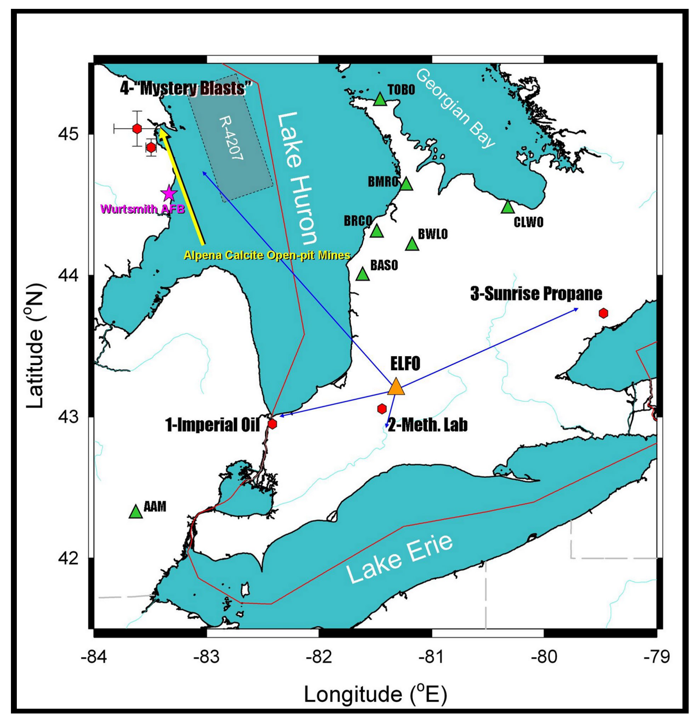
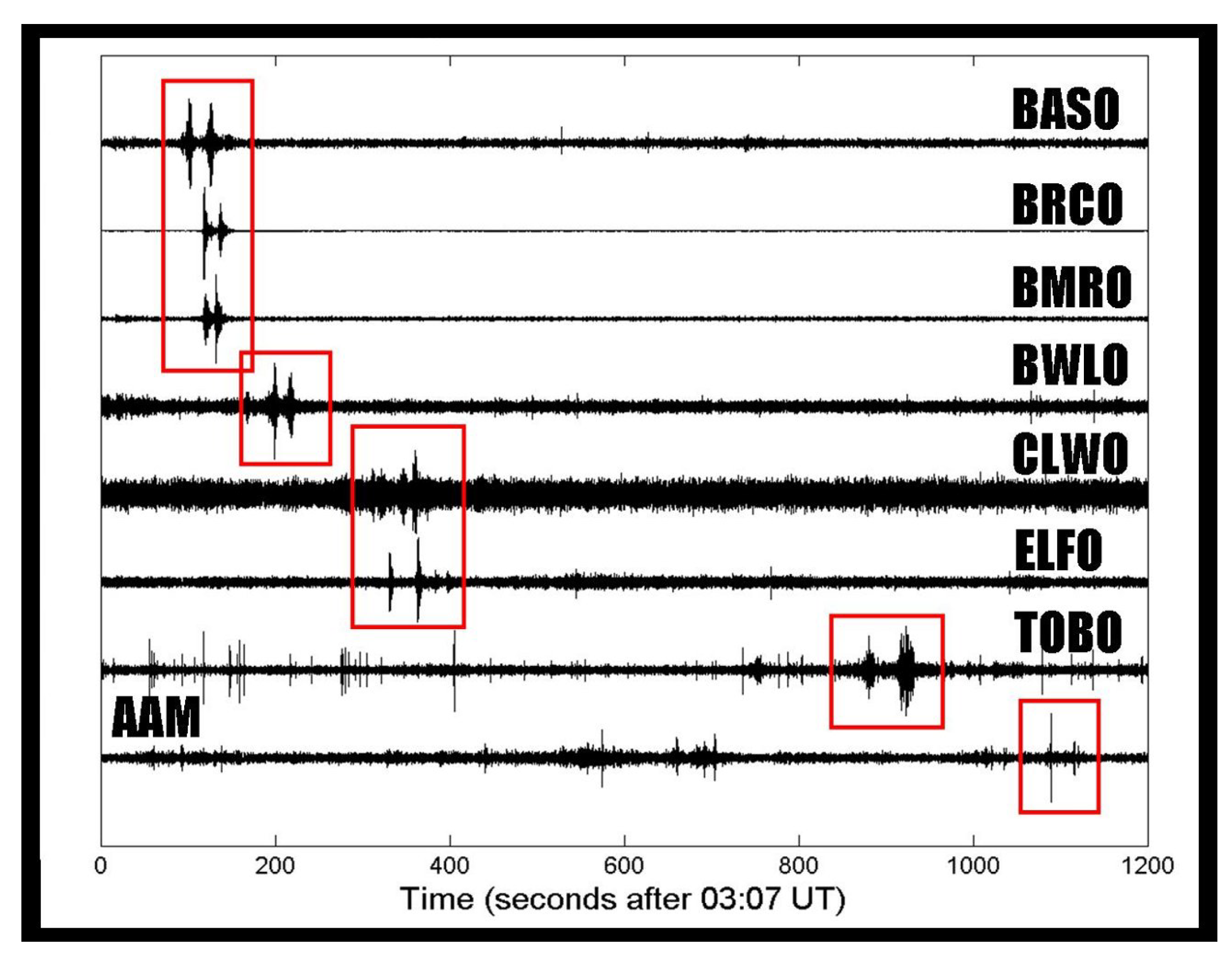
We summarize this section with some important comments. Our prediction for the overpressure (15) for a typical AQN event with $B\simeq {10}^{25}$ at the infrasound frequency (19) suggests that the existing instruments such as ELFO are not sufficiently sensitive to detect such small signals on the level of $\delta p\simeq 0.03$ Pa. Nevertheless, some strong and rare events still can be recorded with existing technology. In particular, it is tempting to identify a single mysterious event recorded by ELFO [7] as the AQN event with very large baryon charge $B\simeq {10}^{27}$, see Appendix A with detailed arguments. Here we just highlight this reasoning.

The radius of the nugget scales as $R\sim B^{1/3}$, which effectively leads to an increase in the number of annihilation events for larger nuggets, which eventually releases higher energy output per unit length as Equation (9) states. Therefore, the intensity of the event scales correspondingly. The powerful explosion recorded by ELFO with overpressure on the level $\delta p\simeq 0.3$ Pa is consistent with the AQN annihilation event with large $B\simeq {10}^{27}$. Such intense events are relatively rare ones according to (4) and (5) as the frequency of appearance is proportional to $f(B)\sim B^{-\alpha }$ with $\alpha$ ≃ (2–2.5). It might be a part of an explanation of why this area has observed a single event in 10 years rather than observing similar events much more often.

It is obvious that we need much more statistics for systematic studies of relatively small but frequent typical events with $B\simeq {10}^{25}$. In the next section we present a possible design of an instrument which could be sufficiently sensitive to infrasound and seismic signals to fulfill this goal. If our proposal turns out to be successful, it will be possible to routinely record a large number of such events which manifest themselves in the form of the infrasonic and seismic signals, while the optical synchronized cameras may not see any light from these events. Infrasonic signals must be always accompanied by sound and seismic waves as discussed above, which can be routinely recorded by conventional seismic stations. These events should demonstrate the daily and annual modulations as the source for these events is the dark matter galactic wind.

4. Detection Strategy and Possible Instruments

As mentioned in the previous section, the sensitivity of instruments similar to ELFO is insufficient to record relatively small events in the atmosphere which occur approximately once a day in an area of ${(100\mathrm{km})}^2$ with $\delta p\simeq 0.01$ Pa and frequency $\nu \simeq 5$ Hz. In this section, we suggest several possible designs of instruments which maybe sufficiently sensitive to detect signals from common small AQNs with $B\sim {10}^{25}$. One should emphasize that the present section should be considered a proposal for future studies where different approaches are being advocated. At this point, we do not know if any of these ideas can be realized in practise. However, we think these new ideas should be explicitly stated, so that researchers from various communities could consider searching for AQN dark matter.

We start the overview with a promising recent development, Distributed Acoustic Sensing (DAS), which is becoming a conventional tool for seismic and other applications, see, for example, [26,27,28,29] and references therein. The basic idea of these activities can be explained as follows. It has been known for quite sometime that distributed optical fiber sensors are capable of measuring the signals at thousands of points simultaneously using an unmodified optical fiber as the sensing element. The recent development is that the DAS is capable of measuring strain changes at all points along the optical fiber at acoustic frequencies, which is crucial for our studies of the acoustic waves emitted due to the AQN passage.

The main element of the DAS technology is that a pulse of light is sent into optical fiber and, through scattering in the glass, a small amount of the incident light is scattered back towards the sensing unit. The key point is that the DAS is capable of determining from this scattered light, a component which indicates changes in the local axial strain along the fibre. It has been shown that this technology is capable of detecting signals at frequencies as low as 8 mHz and as high as 49.5 kHz with sensitivity at the level of $\delta p\sim 0.1\mathrm{mBar}\approx 10\mathrm{Pa}$ [26] which is more than sufficient for our purposes for $\delta p$ as estimated in (24) and typical frequencies in kHz band as estimated in (26). Furthermore, it has been shown that using an amplifier chain one can extend the range of DAS units to 82 km, while maintaining high signal quality [26]. Such a long range on the scale of 100 km matches well with what is needed for AQN-passage detection. Indeed, we anticipate approximately one event per day per an area of ${(100\mathrm{km})}^2$ according to (5) reviewed in Section 2. An important point is that such studies can in principle detect not only the intensity and the frequency of the sound wave, but also the direction of the source. We note that networks of optical-fiber telecommunication cables cover a significant part of the Earth’s surface.

We anticipate that the main problem with DAS will be separation of the AQN signal from the seismic noise and numerous spurious events. We discuss one of the possibilities to separate the signal from a much larger noise below. The main point is that the AQN signal must show the annual (29) and daily (30) modulations characteristic of the dark matter galactic wind, in contrast with much more numerous and much more intense random events.

The phase of an optical wave propagating over a distance in a fiber accumulates effects of external perturbation and is highly sensitive to these perturbations. The changes of the phases are detected by a network of synchronised atomic clocks and optical cavities. The original idea was to detect transient effects produced by clumps of low-mass dark matter and by passing topological defects. Here, we suggest that such networks may also be sensitive to the blast waves produced by AQN.

The blast wave pressure $\delta p$ produces a minor change of the optical fiber index of refraction and changes the optical length, $\delta L_{\mathrm{opt}}$. This leads to a change in the phase of order $\varphi =\delta L_{\mathrm{opt}}/\lambda$, where the wavelength $\lambda \sim 500$ nm = $0.5\times {10}^{-6}$ m. The relative accuracy of the best atomic clocks has surpassed ${10}^{-18}$, but this requires a long observation time. As an estimate of the best current sensitivity we may take $\delta L\sim {10}^{-19}$ m as in LIGO and VIRGO gravitational wave detectors. This very high sensitivity indicates that the main problem here is the separation of the AQN signal from the seismic noise. One of possibilities to separate the signal from a much larger noise was suggested in [30].

The basic idea of [30] can be explained as follows. The AQN flux is given by (5) if averaged over very long period of time, longer than a year. However, due to the relative motion and orienation of the Sun, Earth and the galaxy, the AQN flux, as that of any other dark mater particle, receives the time-dependent factor $A_{(\mathrm{a})}(t)$ representing the annual modulation which is defined as follows:

$$A_{(\mathrm{a})}(t)\equiv [1+{\kappa }_{(\mathrm{a})}cos{\Omega }_a(t-t_0)],$$

(29)

where ${\Omega }_a=2\pi {\mathrm{yr}}^{-1}\approx$$2\pi ·32$ nHz is the angular frequency of the annual modulation and label “a” in ${\Omega }_a$ stands for annual. The ${\Omega }_a{t}_0$ is the phase shift corresponding to the maximum on 1 June and minimum on 1 December for the standard galactic DM distribution, see [31,32]. Similar daily modulations are also known to occur [33] and can be represented as follows:

$$A_{(\mathrm{d})}(t)\equiv [1+{\kappa }_{(\mathrm{d})}cos({\Omega }_{d}t-{\varphi }_0)],$$

(30)

where ${\Omega }_d=2\pi {\mathrm{day}}^{-1}$$\approx 2\pi ·11.6$ μHz is the angular frequency of the daily modulation, while ${\varphi }_0$ is the phase shift similar to ${\Omega }_a{t}_0$ in (29). It can be assumed to be constant on the scale of days. However, it actually slowly changes with time due to the variation of the direction of DM wind with respect to the Earth. The modulation coefficients ${\kappa }_{(\mathrm{a})}$ and ${\kappa }_{(\mathrm{d})}$ have been computed in the AQN model in [33].

The idea advocated in [30] is to fit the data to the modulation Formulae (29) and (30), even if the noise is large and exceeds the expected signal. The key point here is the statistics factor and accumulation of the signal for a long period of time assuming that the noise can be treated as being random in contrast with signal being characterized by well defined frequencies ${\Omega }_a$ and ${\Omega }_d$. A hope is to discover the annual (29) and daily (30) modulations by recording a large number of AQN events which represent the dark matter galactic wind in this specific model.

This idea of separation of the signal from the spurious effects should work even if the noise also has the same periodicity of 24 h such as the temperature variation. The point is that the phase shift ${\varphi }_0$ of the signal and the temperature variation do not coincide. Furthermore, one could study the variation of the phase shift ${\varphi }_0$ within one season to discriminate the genuine signals from the noise as the DM signal slowly drifts with the season while the noise (such as temperature) does not.

Another way to discriminate the signal from the noise is to study the synchronized signals and time delays by different detectors from a single AQN propagating in atmosphere. This approach may also reconstruct the AQN’s trajectory as argued in [34].

A specific signal from AQN tracks is very different from the ordinary seismic noise and earthquakes. Therefore, AQN signals may, in principle, be detected by an existing network of seismic stations. In addition to optical-fiber based methods, it may be possible to search for the AQN-passage signatures also in the large volumes of existing historical data from networks of seismometers [35].

We would like to briefly mention other possibilities for the AQN detection, see also relevant references in Section 2 leading to the constraints (3). The AQN produce only a small amount of visible light as we already mentioned. However, the emitted X-rays will be absorbed and heat the atmosphere along the track on scales of order L as Equation (12) suggests. It may produce vapor tracks along the AQN path.Therefore, one may try to observe infrared radiation from AQN tracks using infrared telescopes being synchronized with infrasonic detectors and all-sky cameras. Similarly, the AQN tracks also produce microwave and radio wave radiation which may be detected by radio telescopes which can be also synchronized with infrasonic and all sky cameras.

Furthermore, while an AQN itself is only $R\simeq {10}^{-5}$ cm in size, nevertheless, it may leave larger and noticeable cracks along its path in solids as instantaneous defect creation and temperature increase occur on a cm scale according to (22). The cracks could be sufficiently large to be observed. A search for AQN annihilation tracks could also be performed in old rocks and Antarctic ice.

Finally, one more possibility to study the long ranged signals which could be produced by the AQN traversing the Earth atmosphere is to search for signals similar to the ones which are normally attributed to the ultra high energy cosmic rays. In fact, the recent unusual mysterious bursts recorded by the Telescope Array Experiment might be precisely those types of events as argued in [36]. The very puzzling multi-modal clustering events recorded by the HORIZON 10T collaboration may be also related to the AQN traversing the atmosphere as argued in [37].

5. Conclusions

The main results of the present work can be summarized as follows:

1. We argue that an AQN propagating in the Earth’s atmosphere generates infrasonic waves. We estimated the intensity (15) and spectral features (19) of these waves for a typical AQN event with $B\simeq {10}^{25}$;

2. We also performed similar estimates for an AQN propagating inside the Earth;

3. We propose a detection strategy to search for a signal generated by a typical relatively small AQN event with $B\simeq {10}^{25}$ by using distributed acoustic sensing as existing instruments are not sufficiently sensitive to detect such signals;

4. Specific signals from AQN passage may also be detected with a variety of alternative techniques, for instance, with an existing network of seismic stations (or even by analyzing the already existing data) or by analyzing specific synchronized events which may mimic the Ultrahigh Energy Cosmic Rays, as mentioned at the end of Section 4;

5. We further speculate that the mysterious explosion which occurred on 31 July 2008 and which was properly recorded by the dedicated Elginfield Infrasound Array [7] might be a good candidate for an AQN-annihilation event with a large $B\simeq {10}^{27}$ as our basic estimates for the overpressure (A1) and the frequency (A2) are tantalizingly close to the signal recorded by ELFO.

One should emphasize that our estimates are based on the parameters of the AQN model which were fixed long ago for completely different reasons, namely, to explain various different phenomena occurring in drastically different environments, as reviewed in Section 2.

Why should one take this (AQN) model seriously? A simple answer is as follows. Originally, this model was invented to explain the observed relation ${\Omega }_{\mathrm{DM}}\sim {\Omega }_{\mathrm{visible}}$ where the “baryogenesis” framework is replaced with a “charge-separation” paradigm, as reviewed in the Introduction and in Section 2. This model is shown to be consistent with all available cosmological, astrophysical, satellite, and ground-based constraints, where AQNs could leave a detectable electromagnetic signature with one and the same set of parameters. Furthermore, it was shown that AQNs could have been formed and could have survived the harsh environment of the early universe. Therefore, AQNs deserve to be considered a viable DM candidate. Finally, the same AQN framework may also explain a number of other (naively unrelated) observed phenomena as discussed in a recent review [6].

References

1. Zhitnitsky, A.R. ‘Nonbaryonic’ dark matter as baryonic colour superconductor. J. Cosmol. Astropart. Phys. 2003, 10, 10. [Google Scholar] [CrossRef] [Green Version]
2. Witten, E. Cosmic separation of phases. Phys. Rev. D 1984, 30, 272–285. [Google Scholar] [CrossRef]
3. Farhi, E.; Jaffe, R.L. Strange matter. Phys. Rev. D 1984, 30, 2379–2390. [Google Scholar] [CrossRef]
4. De Rujula, A.; Glashow, S.L. Nuclearites—A novel form of cosmic radiation. Nature 1984, 312, 734–737. [Google Scholar] [CrossRef] [Green Version]
5. Madsen, J. Physics and Astrophysics of Strange Quark Matter. In Hadrons in Dense Matter and Hadrosynthesis; Cleymans, J., Geyer, H.B., Scholtz, F.G., Eds.; Lecture Notes in Physics; Springer: Berlin, Germany, 1999; Volume 516, p. 162. [Google Scholar] [CrossRef] [Green Version]
6. Zhitnitsky, A. Axion quark nuggets. Dark matter and matter–antimatter asymmetry: Theory, observations and future experiments. Mod. Phys. Lett. A 2021, 36, 2130017. [Google Scholar] [CrossRef]
7. The Elginfield Infrasound Array (ELFO). Meteor Infrasound. Available online: https://aquarid.physics.uwo.ca/research/infrasound/is_mysteriousexplosions.html (accessed on 11 January 2022).
8. Lawson, K.; Liang, X.; Mead, A.; Siddiqui, M.S.R.; Van Waerbeke, L.; Zhitnitsky, A. Gravitationally trapped axions on the Earth. Phys. Rev. D 2019, 100, 043531. [Google Scholar] [CrossRef] [Green Version]
9. Herrin, E.T.; Rosenbaum, D.C.; Teplitz, V.L. Seismic search for strange quark nuggets. Phys. Rev. D 2006, 73, 043511. [Google Scholar] [CrossRef] [Green Version]
10. Zhitnitsky, A. Solar Extreme UV radiation and quark nugget dark matter model. J. Cosmol. Astropart. Phys. 2017, 10, 050. [Google Scholar] [CrossRef] [Green Version]
11. Raza, N.; van Waerbeke, L.; Zhitnitsky, A. Solar corona heating by axion quark nugget dark matter. Phys. Rev. D 2018, 98, 103527. [Google Scholar] [CrossRef] [Green Version]
12. Ge, S.; Lawson, K.; Zhitnitsky, A. Axion quark nugget dark matter model: Size distribution and survival pattern. Phys. Rev. D 2019, 99, 116017. [Google Scholar] [CrossRef] [Green Version]
13. Silber, E.A.; Boslough, M.; Hocking, W.K.; Gritsevich, M.; Whitaker, R.W. Physics of meteor generated shock waves in the Earth’s atmosphere—A review. Adv. Space Res. 2018, 62, 489–532. [Google Scholar] [CrossRef] [Green Version]
14. Zhitnitsky, A. Cold dark matter as compact composite objects. Phys. Rev. D 2006, 74, 043515. [Google Scholar] [CrossRef] [Green Version]
15. Flambaum, V.V.; Zhitnitsky, A.R. Primordial Lithium Puzzle and the Axion Quark Nugget Dark Matter Model. Phys. Rev. D 2019, 99, 023517. [Google Scholar] [CrossRef] [Green Version]
16. Lawson, K.; Zhitnitsky, A.R. The 21 cm absorption line and the axion quark nugget dark matter model. Phys. Dark Univ. 2019, 24, 100295. [Google Scholar] [CrossRef] [Green Version]
17. ReVelle, D. on meteor-generated infrasound. J. Geophys. Res. Planets 1976, 81, 1217. [Google Scholar] [CrossRef]
18. Silber, E.A.; Brown, P.G. Optical observations of meteors generating infrasound—I: Acoustic signal identification and phenomenology. J. Atmos. Sol. Terr. Phys. 2014, 119, 116–128. [Google Scholar] [CrossRef] [Green Version]
19. Silber, E.A.; Brown, P.G.; Krzeminski, Z. Optical observations of meteors generating infrasound: Weak shock theory and validation. J. Geophys. Res. Planets 2015, 120, 413–428. [Google Scholar] [CrossRef] [Green Version]
20. Tanabashi, M. Review of Particle Physics. Phys. Rev. D 2018, 98, 030001. [Google Scholar] [CrossRef] [Green Version]
21. Forbes, M.M.; Zhitnitsky, A.R. WMAP Haze: Directly Observing Dark Matter? Phys. Rev. D 2008, 78, 083505. [Google Scholar] [CrossRef] [Green Version]
22. Forbes, M.M.; Lawson, K.; Zhitnitsky, A.R. The Electrosphere of Macroscopic ‘Quark Nuclei’: A Source for Diffuse MeV Emissions from Dark Matter. Phys. Rev. D 2010, 82, 083510. [Google Scholar] [CrossRef] [Green Version]
23. FjASr, E.; Holt, R.; Horsrud, P.; Raaen, A.; Risnes, R. Chapter 5 Elastic wave propagation in rocks. In Petroleum Related Rock Mechanics, 2nd ed.; FjASr, E., Holt, R., Horsrud, P., Raaen, A., Risnes, R., Eds.; Elsevier: Amsterdam, The Netherlands, 2008; Volume 53, pp. 175–218. [Google Scholar] [CrossRef]
24. Landau, L.D.; Lifshitz, E.M. Fluid Mechanics, 2nd ed.; Butterworth-Heinemann: Oxford, UK, 1987; Volume 6. [Google Scholar] [CrossRef]
25. Absorption Length Calculator. Available online: http://resource.npl.co.uk/acoustics/techguides/seaabsorption/ (accessed on 11 January 2022).
26. Parker, T.; Shatalin, S.; Farhadiroushan, M. Distributed Acoustic Sensing—A new tool for seismic applications. First Break 2014, 32, 61. [Google Scholar] [CrossRef]
27. Daley, T.; Miller, D.E.; Dodds, K.; Cook, P.; Freifeld, B.M. Field testing of modular borehole monitoring with simultaneous distributed acoustic sensing and geophone vertical seismic profiles at Citronelle, Alabama. Geophys. Prospect. 2016, 64, 1318. [Google Scholar] [CrossRef] [Green Version]
28. Jousset, P.; Reinsch, T.; Ryberg, T.; Blanck, H.; Clarke, A.; Aghayev, R.; Hersir, G.P.; Henninges, J.; Weber, M.; Krawczyk, C.M. Dynamic strain determination using fibre-optic cables allows imaging of seismological and structural features. Nat. Commun. 2018, 9, 2509. [Google Scholar] [CrossRef] [PubMed]
29. Ajo-Franklin, J.B.; Dou, S.; Lindsey, N.J.; Monga, I.; Tracy, C.; Robertson, M.; Rodriguez Tribaldos, V.; Ulrich, C.; Freifeld, B.; Daley, T.; et al. Distributed Acoustic Sensing Using Dark Fiber for Near-Surface Characterization and Broadband Seismic Event Detection. Sci. Rep. 2019, 9, 1328. [Google Scholar] [CrossRef] [PubMed] [Green Version]
30. Budker, D.; Flambaum, V.V.; Liang, X.; Zhitnitsky, A. Axion Quark Nuggets and how a Global Network can discover them. Phys. Rev. D 2020, 101, 043012. [Google Scholar] [CrossRef] [Green Version]
31. Freese, K.; Frieman, J.; Gould, A. Signal modulation in cold-dark-matter detection. Phys. Rev. D 1988, 37, 3388–3405. [Google Scholar] [CrossRef] [PubMed] [Green Version]
32. Freese, K.; Lisanti, M.; Savage, C. Colloquium: Annual modulation of dark matter. Rev. Mod. Phys. 2013, 85, 1561–1581. [Google Scholar] [CrossRef] [Green Version]
33. Liang, X.; Mead, A.; Siddiqui, M.S.R.; Van Waerbeke, L.; Zhitnitsky, A. Axion Quark Nugget Dark Matter: Time Modulations and Amplifications. Phys. Rev. D 2020, 101, 043512. [Google Scholar] [CrossRef] [Green Version]
34. Liang, X.; Peshkov, E.; Van Waerbeke, L.; Zhitnitsky, A. Proposed network to detect axion quark nugget dark matter. Phys. Rev. D 2021, 103, 096001. [Google Scholar] [CrossRef]
35. Incorporated Research Institutions for Seismology (IRIS) Network. Available online: https://www.iris.edu/hq/programs/gsn (accessed on 11 January 2022).
36. Zhitnitsky, A. The Mysterious Bursts observed by Telescope Array and Axion Quark Nuggets. J. Phys. G Nucl. Part Phys. 2020. [Google Scholar] [CrossRef]
37. Zhitnitsky, A. Multi-Modal Clustering Events Observed by Horizon-10T and Axion Quark Nuggets. Universe 2021, 7, 384. [Google Scholar] [CrossRef]