Symmetry in the Multidimensional Dynamical Analysis of Iterative Methods with Memory

Abstract

In this paper, new tools for the dynamical analysis of iterative schemes with memory for solving nonlinear systems of equations are proposed. These tools are in concordance with those of the scalar case and provide interesting results about the symmetry and wideness of the basins of attraction on different iterative procedures with memory existing in the literature.

1. Introduction

Iterative methods for solving nonlinear systems of equations are a fundamental tool for solving problems in applied mathematics since in most of the problems it is sometimes complicated or impossible to solve these systems. For this reason, iterative methods are used since, by giving an initial estimate close enough to the solution, they obtain an approximation of the solution.

As mentioned above, it is necessary for the initial estimate to be close to the solution to ensure convergence, but this does not always happen, which is why the dynamical study is becoming increasingly important, since this is how we can see the behaviour of the initial estimations.

The study of the stability of iterative fixed-point methods can be carried out by means of real or complex dynamics tools applied to a rational operator that result from applying the iterative scheme to low-degree polynomials. These dynamical techniques can be used to compare or to deepen known iterative methods, as can be seen in [1,2,3], to analyze the qualitative properties of new iterative methods without memory (see, for example, [4,5,6,7]) or with memory (see, for instant, [8,9]). They also change if the method is multidimensional, as we can see in [8,10,11,12,13,14,15].

In this paper, we are going to lay the foundations for our future work in the study of the dynamics of iterative methods with memory for approximating the solutions of nonlinear systems.

In the first section, we present the theoretical concepts and the obtained results. Then, in the second section, we apply these results to some multidimensional iterative schemes with memory. We choose two different systems to see the behaviour of these iterative schemes.

2. Theoretical Concepts

Let $F\left(x\right)=0$ be a system of nonlinear equations where $F:{\mathbb{R}}^n\to {\mathbb{R}}^n$.

The standard form of an iterative method with memory that uses only two previous iterations to calculate the next one is:

$$x^{(k+1)}=\varphi \left(x^{(k-1)},x^{\left(k\right)}\right),k\ge 1,$$

where $x^{\left(0\right)}$ and $x^{\left(1\right)}$ are the initial estimations.

From here on, we assumed that when introducing memory to the iterative method, the operator $\varphi$ depends not only on $x^{\left(k\right)}$ but also depends on the variable of the previous step, $x^{(k-1)}$, since otherwise a study of the dynamics of a iterative method without memory for systems would be carried out.

A function defined from ${\mathbb{R}}^n$ to ${\mathbb{R}}^n$ cannot have fixed points since to be a fixed point of a function, the point and its image by the function must coincide. Therefore, an auxiliary function O is defined as follows:

$$O\left(x^{(k-1)},x^{\left(k\right)}\right)=\left(x^{\left(k\right)},x^{(k+1)}\right)=\left(x^{\left(k\right)},\varphi \left(x^{(k-1)},x^{\left(k\right)}\right)\right),k=1,2,\dots$$

If $\left(x^{(k-1)},x^{\left(k\right)}\right)$ is a fixed point of O, then

$$O\left(x^{(k-1)},x^{\left(k\right)}\right)=\left(x^{(k-1)},x^{\left(k\right)}\right),$$

and by the definition of O, one has

$$\left(x^{(k-1)},x^{\left(k\right)}\right)=\left(x^{\left(k\right)},x^{(k+1)}\right).$$

Thus, the discrete dynamical system $O:{\mathbb{R}}^n\times {\mathbb{R}}^n\to {\mathbb{R}}^n\times {\mathbb{R}}^n$ is defined as

$$O(z,x)=\left(x,\varphi (z,x)\right),$$

where $\varphi$ is the operator associated with the vectorial iterative method with memory.

Then, a point $(z,x)$ is a fixed point of O if $z=x$ and $x=\varphi (z,x).$ If $(z,x)$ is a fixed point of operator O that does not satisfy $F\left(x\right)=0$, it is called a strange fixed point.

The basin of attraction of a fixed point $(z^{*},x^{*})$ is defined as the set of pre-images of any order such that

$$\mathcal{A}(z^{*},x^{*})=\{(w,y)\in {\mathbb{R}}^{n\times n}:O^m(w,y)\to (z^{*},x^{*}),m\to \infty \}.$$

To study the caracter of the fixed points, we use the following result from [16].

Theorem 1.

Let $G:{\mathbb{R}}^m\to {\mathbb{R}}^m$ be of class ${\mathcal{C}}^2$ and x a fixed point. Let ${\lambda }_1$, ${\lambda }_2$, …, ${\lambda }_m$ be the eigenvalues of $G^{\prime }\left(x\right)$, where $G^{\prime }$ is the Jacobian matrix of G.

• If $|{\lambda }_j|<1$, for $j=1,2,\dots ,m$, then x is attracing.
• If $|{\lambda }_j|=0$, for $j=1,2,\dots ,m$, then x is super attracing.
• If one eigenvalue ${\lambda }_{j_0}$ has $|{\lambda }_{j_0}|>1$, then x is repelling or saddle.
• If $|{\lambda }_j|>1$, for $j=1,2,\dots ,m$, then x is repelling.

If one eigenvalue $\lambda$ of $G^{\prime }\left(x\right)$ satisfies $\left|\lambda \right|=1$, then x is not hyperbolic and we cannot conclude anything about the character of this fixed point.

We want to obtain a more specific result for determining the character of the fixed points $(z,x)$ of operator O. To do this, we calculate the Jacobian matrix of O, denoted by $O^{\prime }$ which has size $2n\times 2n$. The result is matrix

$$O^{\prime }(z,x)=\left(\begin{array}{cccccc}& 0_{n\times n}& & & I_{n\times n}& \\ {\displaystyle \frac{\partial {\varphi }_1}{\partial z_1}}& \dots & {\displaystyle \frac{\partial {\varphi }_1}{\partial z_n}}& {\displaystyle \frac{\partial {\varphi }_1}{\partial x_1}}& \dots & {\displaystyle \frac{\partial {\varphi }_1}{\partial x_n}}\\ ⋮& & ⋮& ⋮& & ⋮\\ {\displaystyle \frac{\partial {\varphi }_n}{\partial z_1}}& \dots & {\displaystyle \frac{\partial {\varphi }_n}{\partial z_n}}& {\displaystyle \frac{\partial {\varphi }_n}{\partial x_1}}& \dots & {\displaystyle \frac{\partial {\varphi }_n}{\partial x_n}}\end{array}\right).$$

We denote the matrices

$${\displaystyle \frac{\partial \varphi }{\partial z}}=\left(\begin{array}{ccc}{\displaystyle \frac{\partial {\varphi }_1}{\partial z_1}}& \dots & {\displaystyle \frac{\partial {\varphi }_1}{\partial z_n}}\\ ⋮& & ⋮\\ {\displaystyle \frac{\partial {\varphi }_n}{\partial z_1}}& \dots & {\displaystyle \frac{\partial {\varphi }_n}{\partial z_n}}\end{array}\right)$$

and

$${\displaystyle \frac{\partial \varphi }{\partial x}}=\left(\begin{array}{ccc}{\displaystyle \frac{\partial {\varphi }_1}{\partial x_1}}& \dots & {\displaystyle \frac{\partial {\varphi }_1}{\partial x_n}}\\ ⋮& & ⋮\\ {\displaystyle \frac{\partial {\varphi }_n}{\partial x_1}}& \dots & {\displaystyle \frac{\partial {\varphi }_n}{\partial x_n}}\end{array}\right).$$

So, matrix $O^{\prime }(z,x)$ is defined as a block matrix

$$O^{\prime }(z,x)=\left(\begin{array}{cc}{0}_{n\times n}& I_{n\times n}\\ {\displaystyle \frac{\partial \varphi }{\partial z}}& {\displaystyle \frac{\partial \varphi }{\partial x}}\end{array}\right).$$

We need to obtain the eigenvalues of the Jacobian matrix $O^{\prime }(z,x)$ evaluated at the fixed points, for determining the character of them (Theorem 1). It is easy to see that

$$\lambda I_{2n\times 2n}-O^{\prime }(z,x)=\left(\begin{array}{cc}\lambda I_{n\times n}& -I_{n\times n}\\ -{\displaystyle \frac{\partial \varphi }{\partial z}}& \lambda I_{n\times n}-{\displaystyle \frac{\partial \varphi }{\partial x}}\end{array}\right).$$

By applying a result of [17] for calculating the determinant of a block matrix, we obtain

$$det\left(\lambda I_{2n\times 2n}-O^{\prime }(z,x)\right)=det\left(\lambda \left(\lambda I_{n\times n}-{\displaystyle \frac{\partial \varphi }{\partial x}}\right)-{\displaystyle \frac{\partial \varphi }{\partial z}}\right).$$

Then, $\lambda$ is an eigenvalue of $O^{\prime }(z,x)$ if

$$det\left(\lambda \left(\lambda I_{n\times n}-{\displaystyle \frac{\partial \varphi }{\partial x}}\right)-{\displaystyle \frac{\partial \varphi }{\partial z}}\right)=0,$$

which is the same as

$$det\left({\lambda }^2{I}_{n\times n}-\lambda {\displaystyle \frac{\partial \varphi }{\partial x}}-{\displaystyle \frac{\partial \varphi }{\partial z}}\right)=0.$$

These calculations are summarized in the following result.

Theorem 2.

The eigenvalues of $O^{\prime }(z,x)$ are those satisfying:

$$det\left({\lambda }^2{I}_{n\times n}-\lambda {\displaystyle \frac{\partial \varphi }{\partial x}}-{\displaystyle \frac{\partial \varphi }{\partial z}}\right)=0.$$

In particular, $\lambda =0$ is an eigenvalue of $O^{\prime }(z,x)$ if 0 is an eigenvalue of ${\displaystyle \frac{\partial \varphi }{\partial z}}$ since

$$0=det\left(-O^{\prime }(z,x)\right)=det\left(-{\displaystyle \frac{\partial \varphi }{\partial z}}\right).$$

Another concept relevant in a dynamical study is the critical points. In this case, we use the following definition of these type of points.

Definition 1.

Vector $(z,x)$ is a critical point of $O(z,x)$ if all the eigenvalues of $O^{\prime }(z,x)$ are 0.

This is a restrictive definition of a critical point since it is usually sufficient that the determinant of the Jacobian matrix cancels out, but in this case, if we do not use the above definition, we obtain critical point surfaces because of the form of the operator.

To study the eigenvalues of $O^{\prime }(z,x)$, we use Theorem 2. In particular, for at least one of the eigenvalues to be 0, it must be satisfied that $\det \left(O^{\prime }(z,x)\right)=0$; this is equivalent to

$$det\left(O^{\prime }(z,x)\right)=det\left(\begin{array}{cc}{0}_{n\times n}& I_{n\times n}\\ {\displaystyle \frac{\partial \varphi }{\partial z}}& {\displaystyle \frac{\partial \varphi }{\partial x}}\end{array}\right)=det\left(-{\displaystyle \frac{\partial \varphi }{\partial z}}\right)={(-1)}^{n}det\left({\displaystyle \frac{\partial \varphi }{\partial z}}\right).$$

From this, we obtain that:

Theorem 3.

The determinant of $O^{\prime }(z,x)$ is zero if and only if it satisfies

$$det\left({\displaystyle \frac{\partial \varphi }{\partial z}}(z,x)\right)=0.$$

3. Experimental Results

In this section, we present the dynamical study of two simple vectorial methods with memory: Kurchatov’s scheme, ref. [18], whose expression is as follows

$$\begin{array}{c}\hfill x^{(k+1)}=x^{\left(k\right)}-{[2x^{\left(k\right)}-x^{(k-1)},x^{(k-1)};F]}^{-1}F\left(x^{\left(k\right)}\right),k=1,2,\dots \end{array}$$

(1)

and Steffensen’s method with memory, ref. [19], whose expression is

$$\begin{array}{cc}\hfill x^{(k+1)}& \hfill =x^{\left(k\right)}-{[x^{\left(k\right)}+{\gamma }^{\left(k\right)}F\left(x^{\left(k\right)}\right),x^{\left(k\right)};F]}^{-1}F\left(x^{\left(k\right)}\right),\hfill \\ \hfill & \hfill \mathrm{where}{\gamma }^{\left(k\right)}=-{[x^{\left(k\right)},x^{(k-1)};F]}^{-1},k=1,2,\dots \hfill \end{array}$$

(2)

This study is performed on two polynomial systems of different degrees.

3.1. Uncoupled Third Order System

We perform this dynamical study on a system of cubical polynomials in order to use graphical tools. However, these results can be easily extended to higher-dimension systems. The system, denoted by $p\left(x\right)=0$, is as follows:

$$\{\begin{array}{}\hfill \mathrm{(3)}& x_1^3-1=0,\hfill \hfill \mathrm{(4)}& x_2^3-1=0,\hfill \end{array}$$

where $(x_1,x_2)\in {\mathbb{R}}^2$. The only root with real components of this systems is $(1,1)$.

We choose a polynomial of degree 3 instead of one of degree 2 as it is usually done in dynamical studies because the polynomial system of second degree gives us an operator that does not depend on the previous iteration $x^{(k-1)}$, so the study is the same as that of a iterative method without memory for solving nonlinear systems.

To make the study simpler, we denote $x^{(k-1)}$ by z and $x^{\left(k\right)}$ by x as was done in the theoretical study.

3.1.1. Kurchatov’s Method

Operator ${\varphi }_K$ of Kurchatov’s method on the cubical system is

$${\varphi }_K(z,x)=\left(\begin{array}{c}{x}_1+\frac{1-x_1^3}{4x_1^2-2x_1{z}_1+z_1^2}\\ x_2+\frac{1-x_2^3}{4x_2^2-2x_2{z}_2+z_2^2}\end{array}\right).$$

(5)

Theorem 4.

The only fixed point of operator $O_K(z,x)=(x,{\varphi }_K(z,x))$ has equal components $z=x=(1,1)$ and has superattractor character.

Proof. 

We calculate matrices ${\displaystyle \frac{\partial {\varphi }_K}{\partial z}}$ and ${\displaystyle \frac{\partial {\varphi }_K}{\partial x}}$ appearing in the dynamical study,

$${\displaystyle \frac{\partial {\varphi }_K}{\partial z}}(z,x)=\left(\begin{array}{cc}-\frac{2\left(x_1^3-1\right)(x_1-z_1)}{{\left(4x_1^2-2x_1{z}_1+z_1^2\right)}^2}& 0\\ 0& -\frac{2\left(x_2^3-1\right)(x_2-z_2)}{{\left(4x_2^2-2x_2{z}_2+z_2^2\right)}^2}\end{array}\right)$$

and

$${\displaystyle \frac{\partial {\varphi }_K}{\partial x}}(z,x)=\left(\begin{array}{cc}\frac{9x_1^2{z}_1^2-12x_1^3{z}_1+12x_1^4-4x_1\left(z_1^3+2\right)+z_1\left(z_1^3+2\right)}{{\left(4x_1^2-2x_1{z}_1+z_1^2\right)}^2}& 0\\ 0& \frac{9x_2^2{z}_2^2-12x_2^3{z}_2+12x_2^4-4x_2\left(z_2^3+2\right)+z_2\left(z_2^3+2\right)}{{\left(4x_2^2-2x_2{z}_2+z_2^2\right)}^2}\end{array}\right).$$

If we evaluate these matrices at the fixed point, we get

$${\displaystyle \frac{\partial {\varphi }_K}{\partial z}}((1,1),(1,1))=\left(\begin{array}{cc}0& 0\\ 0& 0\end{array}\right)$$

and

$${\displaystyle \frac{\partial {\varphi }_K}{\partial x}}((1,1),(1,1))=\left(\begin{array}{cc}0& 0\\ 0& 0\end{array}\right).$$

By Theorem 2, it follows that $det(\lambda I-O_K^{\prime }((1,1),(1,1)))=det\left({\lambda }^{2}I\right)$. From the above relationship it follows that the only eigenvalue associated with the fixed point is $\lambda =0$. So, fixed point $x=z=(1,1)$ is a superattracting point. □

Regarding the critical points of operator $O_K(z,x)$, we have

Theorem 5.

Operator $O_K(z,x)$ has four types of critical points, denoted by $C_i(z,x)$, which have the following form.

The notation of Table 1 is understood in such a way that, for example, the points C2(z, x) are those that verify that $x_1=1$ and $z_2=x_2$, and the other components are arbitrary.

Table 1. Types of points of Kurchatovs’s scheme that are critical points for $p\left(x\right)=0$.

	${\mathit{x}}_1=1$	${\mathit{z}}_1={\mathit{x}}_1$
$x_2=1$	$C_1(z,x)$	$C_3(z,x)$
$z_2=x_2$	$C_2(z,x)$	$C_4(z,x)$

Proof. 

To do this, we calculate the eigenvalues of $O_K^{\prime }(z,x)$ for any point $(z,x)$ and obtain those satisfying the condition that all their eigenvalues are 0.

It is obtained that the critical points are those $z=(z_1,z_2)$ and $x=(x_1,x_2)$ that satisfy these two expressions

$$\begin{array}{cc}\hfill & \hfill \left(x_1^3-1\right)(x_1-z_1)=0\mathrm{and}\left(x_2^3-1\right)(x_2-z_2)=0.\hfill \end{array}$$

(6)

It follows that the 4 types of points defined in Table 1 are critical points of operator $O_K(z,x)$. □

We have that the points of type $C_1(z,x)$ are a preimage of the only fixed point since ${\varphi }_K(z,(1,1))=(1,1)$. We are only going to study the orbit of the points of type $C_2(z,x)$ and $C_4(z,x)$ since the points $C_1(z,x)$ converge to the fixed point for any value of z, and the fixed points of type $C_3(z,x)$ have a symmetrical study to that of the fixed points of type $C_2(z,x)$.

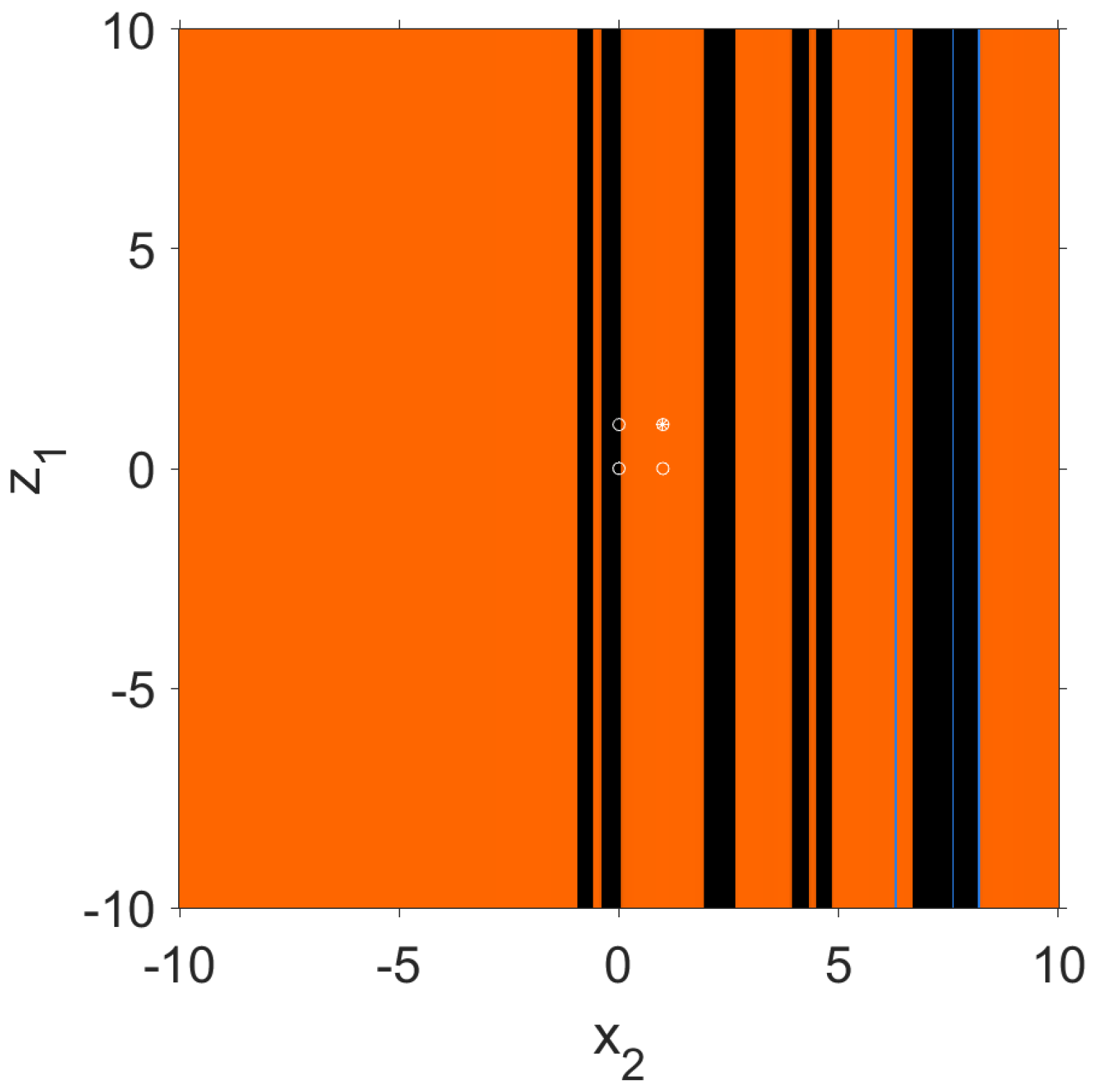
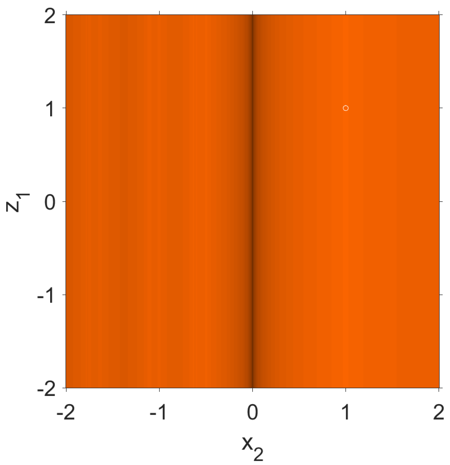
• Operator ${\varphi }_K$ evaluated at the critical points of type $C_2(z,x)$ has the following form

  $${\varphi }_K\left(C_2(z,x)\right)=\left(\begin{array}{c}1\\ x_2+\frac{1-x_2^3}{3x_2^2}\end{array}\right).$$
  The convergence of these points only depends on $x_2$ and $z_1$, as we can see in the expression of ${\varphi }_K$. For this reason, we draw planes of convergence of these points with these two variables.
  Now, we are going to describe how we generate the planes of convergence [4]. To draw these planes of the points of the type $C_2(z,x)$, what we are going to do is to see which of these points belong to the basins of attraction of the attractor fixed points, that is, which of these points converge to the attractor.
  We make a mesh of $400\times 400$ points of the set $[-2,2]\times [-2,2]$. On one of the axes, we have $x_2$, and on the other, $z_1$, and with them we construct our points of type $C_2(z,x)$. We take each of these points $C_2(z,x)$ and apply the operator ${\varphi }_K$ on it. If it converges to the only attractor fixed point, which is $(1,1)$, then we paint it in orange. As convergence criterion, we have used that the distance from the iteration to the fixed point is less than ${10}^{-3}$ in less than 40 iterations. If this is not verified, the mesh point is painted black.
  As can be seen in Figure 1 that we have a slower convergence when $x_2$ approaches the value 0 because of the shape of the operator, but we still have convergence. In the rest of the cases, the convergence to the point $(1,1)$ is clear.

Figure 1. Behaviour of critical points $C_2(z,x)$.

Figure 1. Behaviour of critical points $C_2(z,x)$.

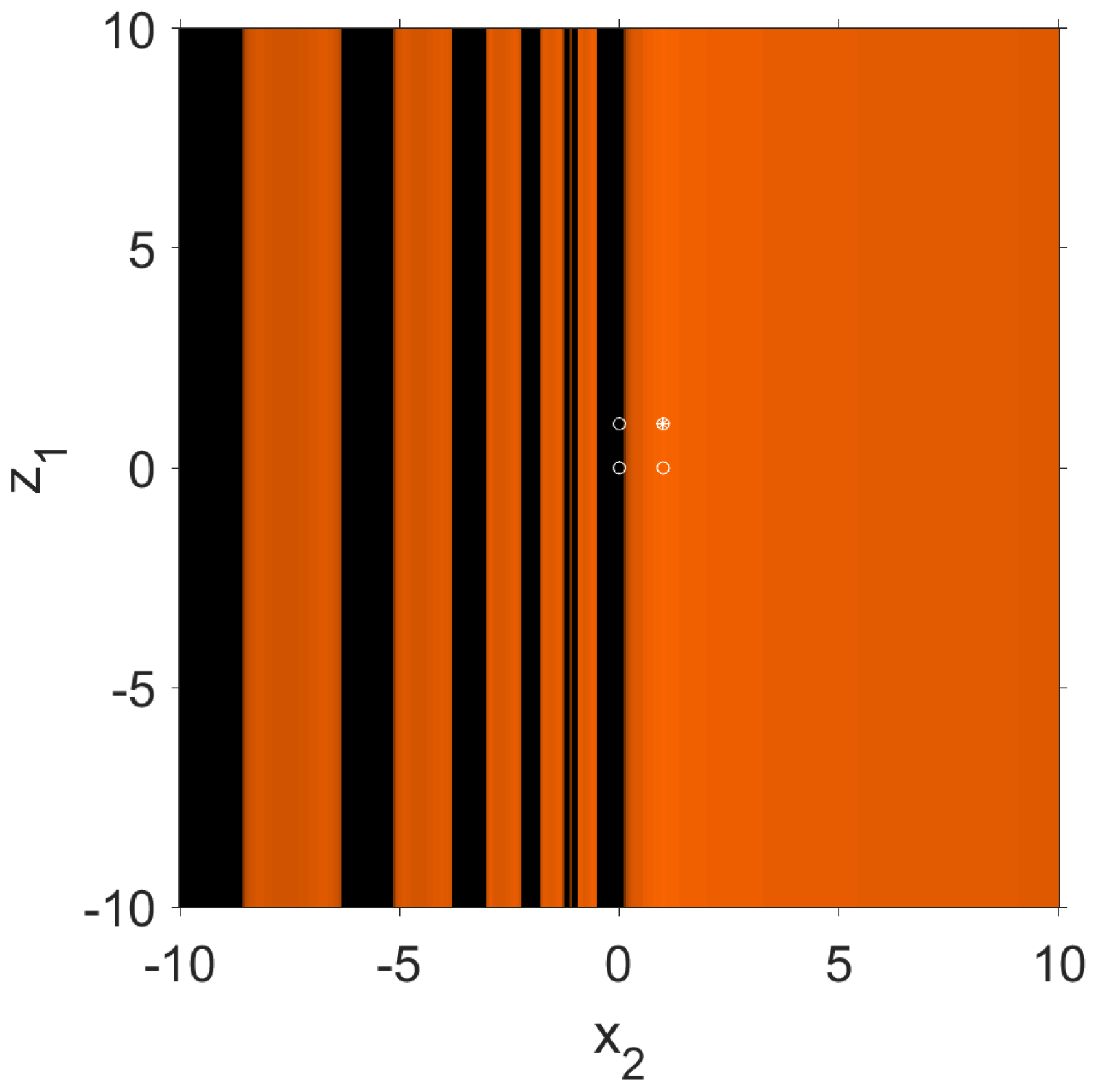
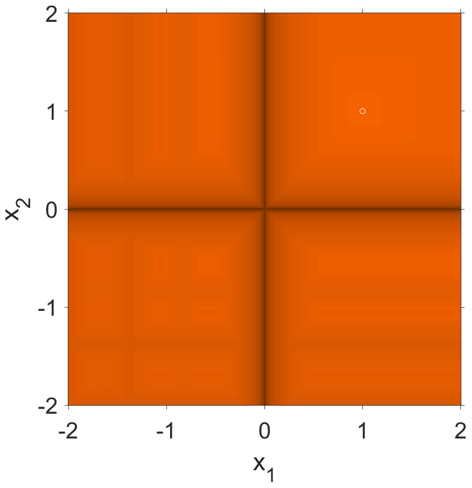
• Next, we evaluate the operator ${\varphi }_K$ at the critical points of type $C_4(z,x)$. In this case, the operator is

  $${\varphi }_K\left(C_4(z,x)\right)=\left(\begin{array}{c}{x}_1+\frac{1-x_1^3}{3x_1^2}\\ x_2+\frac{1-x_2^3}{3x_2^2}\end{array}\right).$$
  In this case, the critical points of type $C_4(z,x)$ depend on variables $x_1$ and $x_2$. For this reason, we draw the convergence plane of the critical points depending on these variables.
  As in the previous case, it is shown in Figure 2 that if any of the variables approach the value 0 we have slow convergence but that in the rest of the points the convergence to the point $(1,1)$ is clear.

Figure 2. Behaviour of critical points $C_4(z,x)$.

Figure 2. Behaviour of critical points $C_4(z,x)$.

To conclude the dynamical study of Kurchatov’s method for this system, let us draw some dynamical planes in order to see the behaviour of the points in general.

To draw these planes, given that we have an operator with 4 variables, what we have done is to select a parameter a, so that $z=x-(a,a)$. We try different values of a to see which one gives the best results. Usually, testing with small values of a gives good results. Thus, our variables would be $x_1$ and $x_2$, and the variables z are a variation of these.

To make the dynamical planes, we have chosen a mesh of $400\times 400$ points, where the chosen point of the mesh is the starting point. We study the orbit of the initial point. If the seed converges to $(1,1)$, it is painted orange, and if it does not converge, it is painted black. We define convergence to the point $(1,1)$ because the distance of the iteration is less than ${10}^{-3}$, and this convergence is realised in, at most, 40 iterations.

We have tested with different values of a over a wide range and obtained that there are the same dynamical plane for different values of a, (Figure 3). As we can see in Figure 3, all initial points converge to the root $(1,1)$ showing the good stability properties of this iterative scheme with memory, even in this multidimensional case.

Figure 3. Dynamical plane of Kurchatov’s scheme for $a=-0.1$.

3.1.2. Steffensen’s Scheme

In this part, we perform the dynamical study of Steffensen’s scheme with memory for system $p\left(x\right)=0$. Operator ${\varphi }_S$ obtained by Steffensen’s method is

$${\varphi }_S(z,x)=\left(\begin{array}{c}{x}_1+\frac{{\left(x_1^3-1\right)}^2}{\left(x_1^2+x_1{z}_1+z_1^2\right)\left({\left(\frac{1-x_1^3}{x_1^2+x_1{z}_1+z_1^2}+x_1\right)}^3-x_1^3\right)}\\ x_2+\frac{{\left(x_2^3-1\right)}^2}{\left(x_2^2+x_2{z}_2+z_2^2\right)\left({\left(\frac{1-x_2^3}{x_2^2+x_2{z}_2+z_2^2}+x_2\right)}^3-x_2^3\right)}\end{array}\right).$$

(7)

Theorem 6.

Operator $O_S(z,x)=(x,{\varphi }_S(z,x))$ has four fixed points, which are

• fixed point $(z,x)=(S_1,S_1)$, with $S_1=(1,1)$,
• strange fixed point $(z,x)=(S_2,S_2)$, being $S_2=(0,0)$,
• strange fixed point $(z,x)=(S_3,S_3)$, being $S_3=(1,0)$,
• strange fixed point $(z,x)=(S_4,S_4)$, with $S_4=(0,1)$.

The strange fixed points are not hyperbolic, and the fixed point $(S_1,S_1)$ is a superattractor point.

Proof. 

In order to study the character of these fixed points, we need to obtain matrices ${\displaystyle \frac{\partial {\varphi }_S}{\partial z}}$ and ${\displaystyle \frac{\partial {\varphi }_S}{\partial x}}$.

We denote by $G{Z}_i(z,x)$ for $i=1,2$ the following expression:

$$G{Z}_i(z,x)=\frac{{\left(x_i^3-1\right)}^2(x_i+2z_i)\left(x_i^2+x_i{z}_i+z_i^2\right)\left(3x_i^2{z}_i+x_i^3+3x_i{z}_i^2+2\right)}{{\left(6x_i^4{z}_i^2+x_i^3\left(6z_i^3+1\right)+3x_i^2\left(z_i^4+z_i\right)+3x_i^5{z}_i+x_i^6+3x_i{z}_i^2+1\right)}^2}.$$

(8)

Thus,

$${\displaystyle \frac{\partial {\varphi }_S}{\partial z}}(z,x)=\left(\begin{array}{cc}G{Z}_1(z,x)& 0\\ 0& G{Z}_2(z,x)\\ \end{array}\right).$$

We denote by $G{X}_i(z,x)$ for $i=1,2$ expression:

$$\begin{array}{cc}G{X}_i(z,x)=& \hfill {\displaystyle \frac{36x_i^4{z}_i^2+x_i^3\left(39z_i^3+7\right)+12x_i^2\left(2z_i^4+z_i\right)+18x_i^5{z}_i}{{\left(6x_i^4{z}_i^2+x_i^3\left(6z_i^3+1\right)+3x_i^2\left(z_i^4+z_i\right)+3x_i^5{z}_i+x_i^6+3x_i{z}_i^2+1\right)}^2}}\hfill \\ & \hfill +{\displaystyle \frac{4x_i^6+6x_i{z}_i^2\left(z_i^3+2\right)+3z_i^3+1}{{\left(6x_i^4{z}_i^2+x_i^3\left(6z_i^3+1\right)+3x_i^2\left(z_i^4+z_i\right)+3x_i^5{z}_i+x_i^6+3x_i{z}_i^2+1\right)}^2}}\hfill \end{array}$$

(9)

Thus,

$${\displaystyle \frac{\partial {\varphi }_S}{\partial x}}(z,x)=\left(\begin{array}{cc}\left(x_1^3-1\right)\left(z_1^3-1\right)G{X}_1(z,x)& 0\\ 0& \left(x_2^3-1\right)\left(z_2^3-1\right)G{X}_2(z,x)\end{array}\right).$$

Let us now obtain the character of the fixed points $(S_i,S_i)$, for $i=1,\dots ,4$.

• For the point associated to $S_1$, the related matrices are

  $${\displaystyle \frac{\partial {\varphi }_S}{\partial z}}(S_1,S_1)=\left(\begin{array}{cc}0& 0\\ 0& 0\end{array}\right)$$

  and

  $${\displaystyle \frac{\partial {\varphi }_S}{\partial x}}(S_1,S_1)=\left(\begin{array}{cc}0& 0\\ 0& 0\end{array}\right).$$
  From Theorem 2, we conclude that the fixed point is super attracting point.
• For the point associated to $S_2$, we obtain

  $${\displaystyle \frac{\partial {\varphi }_S}{\partial z}}(S_2,S_2)=\left(\begin{array}{cc}0& 0\\ 0& 0\end{array}\right)$$

  and

  $${\displaystyle \frac{\partial {\varphi }_S}{\partial x}}(S_2,S_2)=\left(\begin{array}{cc}1& 0\\ 0& 1\end{array}\right).$$
  By applying Theorem 2, the eigenvalues of this point are the values $\lambda$ satisfying

  $$\begin{array}{cc}0=det(\lambda I-O_S^{\prime }(x,z))& \hfill =det\left({\lambda }^{2}I-\lambda {\displaystyle \frac{\partial \rho }{\partial x}}-{\displaystyle \frac{\partial \rho }{\partial z}}\right)\hfill \\ & \hfill ={\lambda }^2{(\lambda -1)}^2.\hfill \end{array}$$

  (10)
  It follows that the eigenvalues are 0 and 1, so we cannot conclude anything about the character of this strange fixed point as it is not hyperbolic.
• For the fixed point associated to $S_3$, the matrices are

  $${\displaystyle \frac{\partial {\varphi }_S}{\partial z}}(S_3,S_3)=\left(\begin{array}{cc}0& 0\\ 0& 0\end{array}\right)$$

  and

  $${\displaystyle \frac{\partial {\varphi }_S}{\partial x}}(S_3,S_3)=\left(\begin{array}{cc}0& 0\\ 0& 1\end{array}\right).$$
  The eigenvalues associated with this fixed point are those $\lambda$ values that satisfy

  $$\begin{array}{cc}0=det(\lambda I-O_S^{\prime }(x,z))& \hfill =det\left({\lambda }^{2}I-\lambda {\displaystyle \frac{\partial \rho }{\partial x}}-{\displaystyle \frac{\partial \rho }{\partial z}}\right)\hfill \\ & \hfill ={\lambda }^3(\lambda -1).\hfill \end{array}$$

  (11)
  It follows that the eigenvalues are 0 and 1, so again the point is not hyperbolic.
• Finally, let us study the character of the fixed point associated with $S_4$. The matrices for this fixed point are

  $${\displaystyle \frac{\partial {\varphi }_S}{\partial z}}(S_4,S_4)=\left(\begin{array}{cc}0& 0\\ 0& 0\end{array}\right)$$

  and

  $${\displaystyle \frac{\partial {\varphi }_S}{\partial x}}(S_4,S_4)=\left(\begin{array}{cc}1& 0\\ 0& 0\end{array}\right).$$
  So the eigenvalues of the fixed point associated with $S_4$ are the values that satisfy

  $$\begin{array}{cc}0=det(\lambda I-O_S^{\prime }(x,z))& \hfill =det\left({\lambda }^{2}I-\lambda {\displaystyle \frac{\partial \rho }{\partial x}}-{\displaystyle \frac{\partial \rho }{\partial z}}\right)\hfill \\ & \hfill ={\lambda }^3(\lambda -1).\hfill \end{array}$$

  (12)
  It follows that the eigenvalues are 0 and 1, so again the point is not hyperbolic. □

Now, let us calculate the critical points.

Theorem 7.

The critical points of operator $O_S(z,x)$ are vectors $z=(z_1,z_2)$ and $x=(x_1,x_2)$, which satisfy that they are of one of the following 16 types, which we denote by $C{S}_i(z,x)$ for $i=1,\dots ,16$. Table 2 is a summary of the different types of critical points we obtain.

Table 2. Types of points of Steffensen’s scheme that are critical points for $p\left(x\right)=0$.

	${\mathit{x}}_1=1$	${\mathit{z}}_1=-\frac{1}{2}{\mathit{x}}_1$	${\mathit{z}}_1=\frac{-3{\mathit{x}}_1^2+\sqrt{-3{\mathit{x}}_1^4-24{\mathit{x}}_1}}{6{\mathit{x}}_1}$	${\mathit{z}}_1=\frac{-3{\mathit{x}}_1^2-\sqrt{-3{\mathit{x}}_1^4-24{\mathit{x}}_1}}{6{\mathit{x}}_1}$
$x_2=1$	$C{S}_1(z,x)$	$C{S}_5(z,x)$	$C{S}_9(z,x)$	$C{S}_{13}(z,x)$
$z_2=-\frac{1}{2}{x}_2$	$C{S}_2(z,x)$	$C{S}_6(z,x)$	$C{S}_{10}(z,x)$	$C{S}_{14}(z,x)$
$z_2=\frac{-3x_2^2+\sqrt{-3x_2^4-24x_2}}{6x_2}$	$C{S}_3(z,x)$	$C{S}_7(z,x)$	$C{S}_{11}(z,x)$	$C{S}_{15}(z,x)$
$z_2=\frac{-3x_2^2-\sqrt{-3x_2^4-24x_2}}{6x_2}$	$C{S}_4(z,x)$	$C{S}_8(z,x)$	$C{S}_{12}(z,x)$	$C{S}_{16}(z,x)$

We are working with systems of equations with real variables, so it is assumed that the critical points have real numbers as their components.

Proof. 

If we define $DG{X}_i(z,x)$, $i=1,2$, as

$$DG{X}_i(z,x)={\lambda }^2-\lambda (x_1^3-1)(z_1^3-1)G{X}_i(z,x)-G{X}_i(z,x),$$

then, we can check that

$$\begin{array}{cc}det(\lambda I-O_S^{\prime }(x,z))& \hfill =det\left({\lambda }^{2}I-\lambda {\displaystyle \frac{\partial {\varphi }_S}{\partial x}}-{\displaystyle \frac{\partial {\varphi }_S}{\partial z}}\right)\hfill \\ & \hfill =det\left(\begin{array}{cc}DG{X}_1(z,x)& 0\\ 0& DG{X}_2(z,x)\end{array}\right).\hfill \end{array}$$

(13)

Additionally, it follows that all eigenvalues are zero if the point $(z,x)$ has one of the forms given in Table 3. □

Table 3. Symmetry relation between $C{S}_i(z,x)$.

$C{S}_2(z,x)$	$C{S}_5(z,x)$
$C{S}_3(z,x)$	$C{S}_9(z,x)$
$C{S}_4(z,x)$	$C{S}_{13}(z,x)$
$C{S}_7(z,x)$	$C{S}_{10}(z,x)$
$C{S}_8(z,x)$	$C{S}_{14}(z,x)$
$C{S}_{12}(z,x)$	$C{S}_{15}(z,x)$

As we can see on Table 3, there is a certain symmetry relation between the following $C{S}_i(z,x)$.

For that reason, and because the operator also satisfies certain symmetry with the components, we only study the behaviour of certain types of points that are critical points.

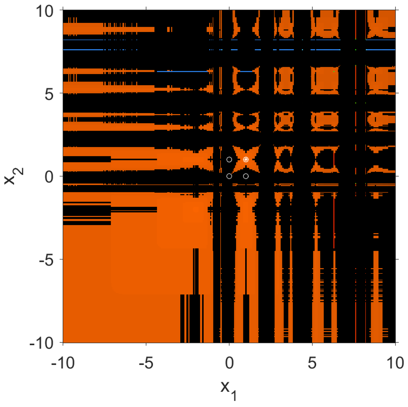
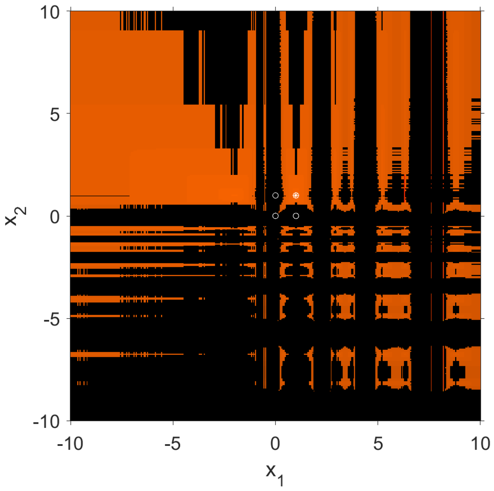
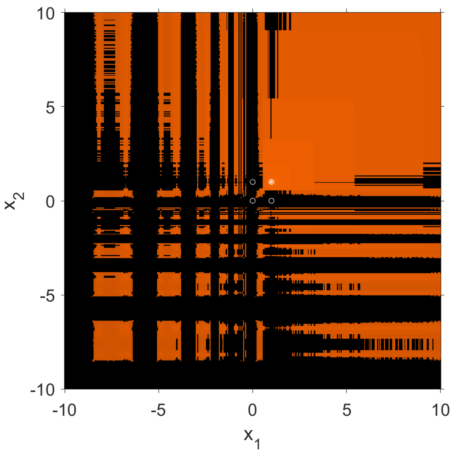
• The asymptotic behaviour of the critical points $C{S}_2(z,x)$ is analysed with the following plane where the convergence to the fixed points is shown in different colours. In this case, if the distance from the iteration to the fixed point is less than ${10}^{-3}$, we say that the iteration is in the basin of attraction of the fixed point. In this case, it is painted orange if the critical point converges to $(S_1,S_1)$, blue if it converges to the strange fixed point $(S_3,S_3)$, red if it converges to the strange fixed point $(S_4,S_4)$ and green if it converges to the point $(S_2,S_2)$. If the points are painted black, they have not converged to any of the fixed points in less than 40 iterations. In this case, we have a fixed value $x_1$, and the value $z_2$ depends on $x_2$, so the variables of the axes are $x_2$ and $z_1$ as shown in Figure 4.

Figure 4. Convergence of the critical points of type $C{S}_2(z,x)$.

Figure 4. Convergence of the critical points of type $C{S}_2(z,x)$.

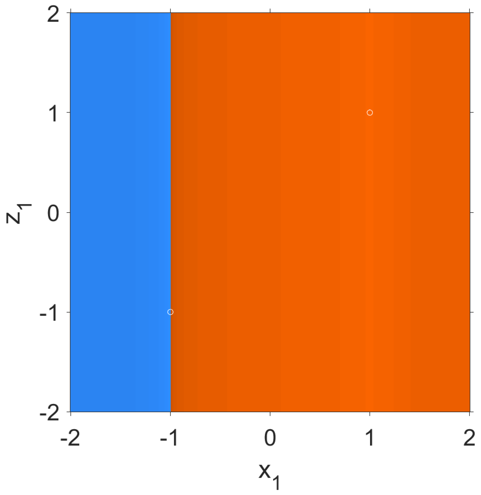
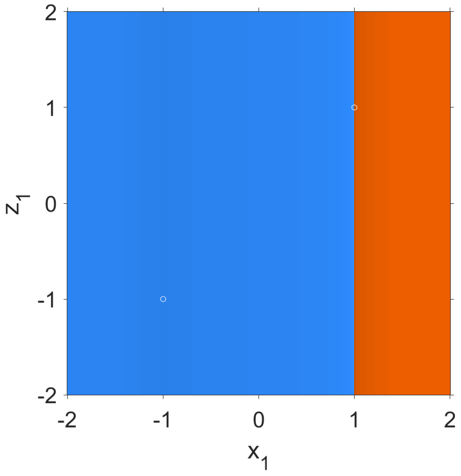
• In a similar way to the previous case, we study the convergence of the critical points of type $C{S}_3(z,x)$ and of type $C{S}_4(z,x)$. In these cases, the value $x_1$ is also fixed and the value $z_2$ depends on $x_2$; for this reason, the variables of the axes are $x_2$ and $z_1$ as in the previous cases and as can be seen in Figure 5. In this case, we have that the behaviour of both types of critical points is the same; for that reason, we only show one dynamical plane.

Figure 5. Convergence of the critical points of type $C{S}_3(z,x)$ and $C{S}_4(z,x)$.

Figure 5. Convergence of the critical points of type $C{S}_3(z,x)$ and $C{S}_4(z,x)$.

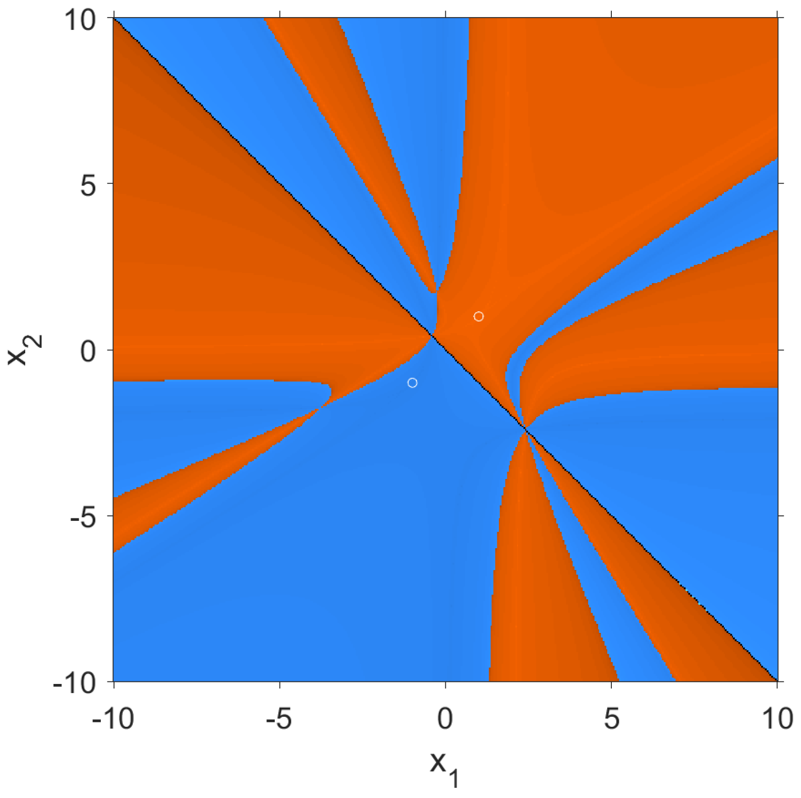
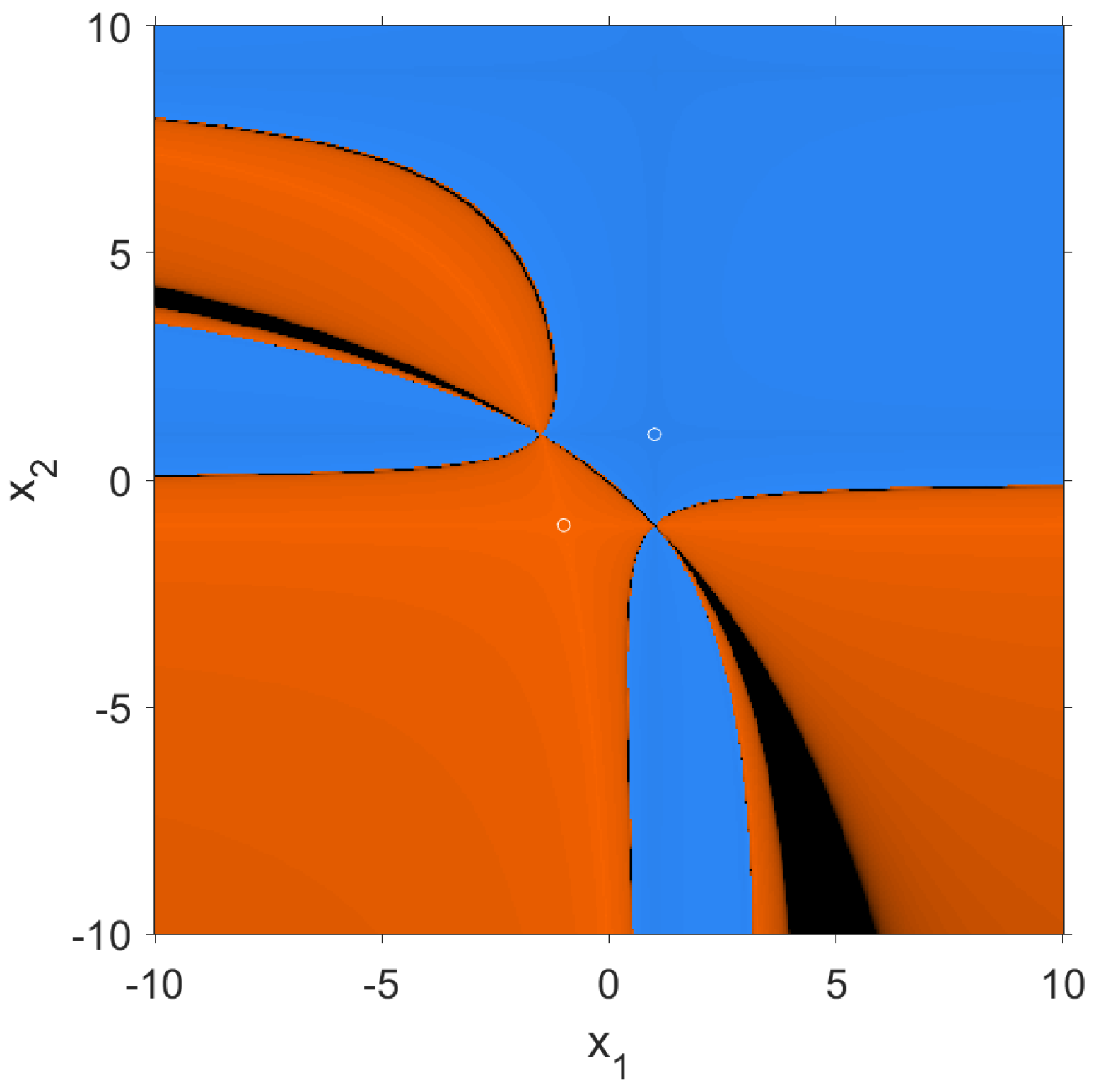
• For the critical points of type $C{S}_6(z,x)$, the convergence study is similar to the previous ones, but in this case none of the variables are fixed, and it is $z_1$ and $z_2$ that depend on $x_1$ and $x_2$, respectively; for this reason, the dynamical plane has as axis variables the values of $x_1$ and $x_2$, as shown in Figure 6.

Figure 6. Convergence of the critical points of type $C{S}_6(z,x)$.

Figure 6. Convergence of the critical points of type $C{S}_6(z,x)$.

• For the critical points of type $C{S}_7(z,x)$ and $C{S}_8(z,x)$, we also have as variables on the axes the values of $x_1$ and $x_2$, as shown in Figure 7. In this case, we have decided to show only one dynamical plane because the behaviour of both types of critical points is the same.

Figure 7. Convergence of the critical points of type $C{S}_7(z,x)$ and $C{S}_8(z,x)$.

Figure 7. Convergence of the critical points of type $C{S}_7(z,x)$ and $C{S}_8(z,x)$.

• For the critical points of type $C{S}_{11}(z,x)$, $C{S}_{12}(z,x)$ and $C{S}_{16}(z,x)$, we also have as variables on the axes the values of $x_1$ and $x_2$. In this case, we have that the behaviour of these 3 types of critical points is the same; for that reason, we only show one dynamical plane (Figure 8).
  

  Figure 8. Convergence of the critical points of type $C{S}_{11}(z,x)$, $C{S}_{12}(z,x)$ and $C{S}_{16}(z,x)$.

3.2. A Coupled Second-Order System

Now, we are going to solve other system that has a more complicated aspect since the variables cannot be separated, that is to say, we do not have that the first component of the operator only depends on the first components of the variables of x and z and the same with the second component; instead, in this case, we have that both components of the operator depend on both components of the vectors. The next system we solve, denoted by $q\left(x\right)=0$, is

$$\{\begin{array}{}\mathrm{(14)}& x_1{x}_2+x_1-x_2-1=0,\mathrm{(15)}& x_1{x}_2-x_1+x_2-1=0,\end{array}$$

where $(x_1,x_2)\in {\mathbb{R}}^2$. The real roots of this system are $(-1,-1)$ and $(1,1)$.

3.2.1. Kurchatov’s Scheme

If we apply the Kurchatov’s scheme to the proposed system, we obtain the following operator:

$${\phi }_K(z,x)=\left(\begin{array}{c}\frac{1-x_2{z}_1+x_1(x_2+z_2)}{2x_1-z_1+z_2}\\ \frac{1-x_2{z}_1+x_1(x_2+z_2}{2x_1-z_1+z_2}\end{array}\right).$$

(16)

Theorem 8.

The only fixed points of the operator $O_K(z,x)=(z,{\phi }_K(z,x))$ are $z=x=(-1,-1)$ and $z=x=(1,1)$, and both have superattractor character.

Proof. 

Now, we calculate the matrices ${\displaystyle \frac{\partial {\phi }_K}{\partial z}}$ and ${\displaystyle \frac{\partial {\phi }_K}{\partial x}}$ to obtain the character of these fixed points.

$${\displaystyle \frac{\partial {\phi }_K}{\partial z}}(z,x)=\left(\begin{array}{cc}\frac{x_1(z_2-x_2)-x_2{z}_2+1}{{(2x_1-z_1+z_2)}^2}& \frac{2x_1^2-x_1(x_2+z_1)+x_2{z}_1-1}{{(2x_1-z_1+z_2)}^2}\\ \frac{x_1(z_2-x_2)-x_2{z}_2+1}{{(2x_1-z_1+z_2)}^2}& \frac{2x_1^2-x_1(x_2+z_1)+x_2{z}_1-1}{{(2x_1-z_1+z_2)}^2}\end{array}\right)$$

and

$${\displaystyle \frac{\partial {\phi }_K}{\partial x}}(z,x)=\left(\begin{array}{cc}\frac{x_2(z_1+z_2)-z_1{z}_2+z_2^2-2}{{(2x_1-z_1+z_2)}^2}& \frac{x_1-z_1}{2x_1-z_1+z_2}\\ \frac{x_2(z_1+z_2)-z_1{z}_2+z_2^2-2}{{(2x_1-z_1+z_2)}^2}& \frac{x_1-z_1}{2x_1-z_1+z_2}\end{array}\right).$$

If we evaluate the previous matrices in the fixed points, we obtain in both cases that both are the matrix that all the components are 0. So, by Theorem 2, both eigenvalues are 0 for all the fixed points. For that reason, both fixed points are super attracting points. □

Theorem 9.

Operator $O_K(z,x)=(z,{\phi }_K(z,x))$ has two types of points that are critical points. These points have one of the following two structures:

• $C_{+}(z,x)=(z_1,z_2,x_1,x_2)$ where $z_2=-x_1+\sqrt{2-x_1^2}+z_1$.
• $C_{-}(z,x)=(z_1,z_2,x_1,x_2)$ where $z_2=-x_1-\sqrt{2-x_1^2}+z_1$.

Proof. 

As we can see,

$$\begin{array}{cc}\hfill det(\lambda I-O_K^{\prime }(z,x))& \hfill =det\left({\lambda }^{2}I-\lambda \frac{\partial {\phi }_K}{\partial x}-\frac{\partial {\phi }_K}{\partial x}\right).\hfill \end{array}$$

(17)

By the form of $\frac{\partial {\phi }_K}{\partial x}$ and $\frac{\partial {\phi }_K}{\partial x}$, we can see that all the eigenvalues are zero if

$$x_1-x_2=0\mathrm{and}{(z_2-z_1+x_1)}^2=2-x_1^2.$$

□

Let us draw the orbit of these critical points. In this case, we draw on the abscissa axis the values of $x_1$, which is the same value as $x_2$, and we draw on the other axis the value of $z_1$ since $z_2$ is obtained from $x_1$ and $z_2$.

To generate these convergence planes of the points of type $C_{+}(z,x)$, we are going to see which of these points belong to the basins of attraction of the attractor fixed points, that is, which of these points converge to the attractor fixed points.

To do this, we make a mesh of $400\times 400$ points of the set $[-2,2]\times [-2,2]$. We made sure that increasing the set did not alter the behaviour. On one of the axes, we have the variable $x_1$, and on the other, the variable $z_1$, and with these variables we construct our points of type $C_{+}(z,x)$. We take each of these points of type $C_{+}(z,x)$, and we apply our operator $\phi$ on them.

If this initial point converges to $(1,1)$, we paint it in orange, and if converges to $(-1,-1)$, we paint it in blue. As convergence criteria, we have that the distance from the iteration to the fixed point is less than ${10}^{-3}$ in less than 40 iterations. If this is not verified, we paint it in black.

Figure 9 shows the plane of convergence for the points of type $C_{+}(z,x)$.

Figure 9. Convergence of the critical points of type $C_{+}(z,x)$.

In the same way that the plane of convergence of the points of type $C_{+}(z,x)$ is generated, we generate the plane of convergence of the points of type $C_{-}(z,x)$, which is shown in Figure 10.

Figure 10. Convergence of the critical points of type $C_{-}(z,x)$.

We observe in this planes of convergence, Figure 9 and Figure 10, that global convergence to the roots of the system exists.

To conclude the dynamical study of the Kurchatov method for this system, we draw some dynamical planes in order to see the behaviour of the points in general. To draw these planes, given that we have an operator with 4 variables, what we have done is to select a parameter a, so that $z=x-(a,a)$. Thus, our variables would be $x_1$ and $x_2$, and the variables z are a variation of these.

To make the dynamical planes, we have chosen a mesh of $400\times 400$ points. If the initial point converges to the point $(1,1)$, it is painted orange; if it converges to point $(-1,-1)$, it is painted blue; and if it does not converge to any point, is painted black.

We have tested with different values of a over a wide range and obtained that there are similar dynamical planes for different values of a; for that reason, we only show Figure 11. As we can see on this figure, we have that all initial estimation converge to the roots of the polynomial.

Figure 11. Dynamical plane of Kurchatov’s scheme with $a=0.1$.

3.2.2. Steffensen’s Scheme

If we apply Steffensen’s scheme with memory to system $q\left(x\right)=0$, we obtain the following operator

$${\theta }_S(z,x)=\left(\begin{array}{c}\frac{2x_1^2{x}_2+x_1{x}_2{z}_2+x_1-x_2+z_2}{2x_1^2+x_1(x_2+z_2)+x_2{z}_2-1}\\ \frac{2x_1^2{x}_2+x_1{x}_2{z}_2+x_1-x_2+z_2}{2x_1^2+x_1(x_2+z_2)+x_2{z}_2-1}\end{array}\right).$$

(18)

Theorem 10.

The operator $O(z,x)=(x,{\theta }_S(z,x))$ has three fixed points, that is,

• $z=x=(-1,-1)$, which is a superattractor point.
• $z=x=(1,1)$, which is a superattractor point.
• $z=x=(0,0)$, which is a strange fixed point and not hyperbolic.

Proof. 

Let us calculate the matrices ${\displaystyle \frac{\partial {\theta }_S}{\partial z}}$ and ${\displaystyle \frac{\partial {\theta }_S}{\partial x}}$ to obtain the character of the fixed points.

$${\displaystyle \frac{\partial {\theta }_S}{\partial z}}(z,x)=\left(\begin{array}{cc}0& -\frac{\left(x_1^2-1\right)\left(x_2^2-1\right)}{{\left(2x_1^2+x_1(x_2+z_2)+x_2{z}_2-1\right)}^2}\\ 0& -\frac{\left(x_1^2-1\right)\left(x_2^2-1\right)}{{\left(2x_1^2+x_1(x_2+z_2)+x_2{z}_2-1\right)}^2}\end{array}\right),$$

(19)

$${\displaystyle \frac{\partial {\theta }_S}{\partial x}}(z,x)=\left(\begin{array}{cc}\frac{\left(x_2^2-1\right)\left(2x_1^2+4x_1{z}_2+z_2^2+1\right)}{{\left(2x_1^2+x_1(x_2+z_2)+x_2{z}_2-1\right)}^2}& \frac{\left(x_1^2-1\right)\left(4x_1^2+4x_1{z}_2+z_2^2-1\right)}{{\left(2x_1^2+x_1(x_2+z_2)+x_2{z}_2-1\right)}^2}\\ \frac{\left(x_2^2-1\right)\left(2x_1^2+4x_1{z}_2+z_2^2+1\right)}{{\left(2x_1^2+x_1(x_2+z_2)+x_2{z}_2-1\right)}^2}& \frac{\left(x_1^2-1\right)\left(4x_1^2+4x_1{z}_2+z_2^2-1\right)}{{\left(2x_1^2+x_1(x_2+z_2)+x_2{z}_2-1\right)}^2}\end{array}\right).$$

(20)

For the fixed points associated with the roots, both matrices are the zero matrix. So, by Theorem 2, both eigenvalues are 0. Then, the fixed points associated with the roots are super attracting points. Let see what happens to the strange fixed point. The matrices are

$${\displaystyle \frac{\partial {\theta }_S}{\partial z}}((0,0),(0,0))=\left(\begin{array}{cc}0& -1\\ 0& -1\end{array}\right),$$

(21)

$${\displaystyle \frac{\partial {\theta }_S}{\partial x}}((0,0),(0,0))=\left(\begin{array}{cc}-1& 1\\ -1& 1\end{array}\right).$$

(22)

By Theorem 2, the eigenvalues for that strange fixed point are the values $\lambda$ that satisfy the following equation:

$$\begin{array}{cc}\hfill det(\lambda I-O_S^{\prime }(z,x))& \hfill =det\left({\lambda }^{2}I-\lambda {\displaystyle \frac{\partial {\theta }_S}{\partial x}}-{\displaystyle \frac{\partial {\theta }_S}{\partial z}}\right)={\lambda }^2({\lambda }^2+1)=0.\hfill \end{array}$$

(23)

So, the eigenvalues are $\pm i$ and 0. We cannot determine the character of that strange fixed-point non-hyperbolic. □

Theorem 11.

Operator $O_S(z,x)=(x,{\theta }_S(z,x))$ has six types of critical points. These types of points are:

All these points are preimages of one of the fixed points.

Proof. 

Since

$$\begin{array}{cc}det(\lambda I-O_S^{\prime }(z,x))& ={\lambda }^4+{\lambda }^2{\displaystyle \frac{(-1+x_1^2)(-1+x_2^2)-\lambda x_2^2}{{(-1+2x_1^2+x_2{z}_2+x_1(x_2+z_2))}^2}}\hfill \\ & +{\lambda }^3{\displaystyle \frac{x_1^2(7-4x_1^2-2x_2^2)-4x_1(-2+x_1^2+x_2^2)z_2-(-2+x_1^2+x_2^2)z_2^2}{{(-1+2x_1^2+x_2{z}_2+x_1(x_2+z_2))}^2}}\hfill \end{array}$$

(24)

Then, all the eigenvalues are zero, if $(z,x)$ has one of the types shown in Table 4.

Table 4. Types of points of Steffensen’s scheme that are critical points for $q\left(x\right)=0$.

	${\mathit{x}}_1=1$	${\mathit{x}}_1=-1$	${\mathit{z}}_2=-{\mathit{x}}_2-2{\mathit{x}}_1$
$x_2=1$	$C{P}_1(z,x)$ if $z_2\ne -3$		$C{P}_5(z,x)$ if $|x_1|\ne 1$
$x_2=-1$		$C{P}_2(z,x)$ if $z_2\ne 3$	$C{P}_6(z,x)$ if $|x_1|\ne 1$
$z_2=-1-2x_1$	$C{P}_3(z,x)$ if $x_2\ne -1$
$z_2=1-2x_1$		$C{P}_4(z,x)$ if $x_2\ne 1$

• Since $\theta$ evaluated at the $C{P}_2(z,x)$, $C{P}_4(z,x)$ and $C{P}_6(z,x)$ points is $(-1,-1)$, then those types of critical points belongs to the basin of attraction of $(-1,-1)$.
• Since $\theta$ evaluated at the $C{P}_1(z,x)$, $C{P}_3(z,x)$ and $C{P}_5(z,x)$ points is $(1,1)$, then those types of critical points belongs to the basin of attraction of $(1,1)$.

□

Below, we draw a dynamical plane for the Steffensen’s scheme with memory in the same way as was done for the Kurchatov’s scheme. In Figure 12, we can see a black region; that is because we have slow convergence to the roots in that region since there are no critical points outside the basins of attraction of the roots, so there cannot be convergence to any point other than the roots. Here, we also tried different values for the parameter a, and similar results were obtained, although the larger the parameter was, the more slowly convergence zone increased.

Figure 12. Dynamical plane of Steffensen’s method with $a=-0.1$.

4. Conclusions

The design of new vectorial iterative schemes with memory for solving nonlinear problems is a developing area of numerical analysis that has expanded in recent years. These methods can be numerically checked, but, until now, there were no possibility of analyzing their qualitative performance as all the existing techniques, including both complex and real discrete dynamics, were not defined to overcome the high dimensionality of the rational functions involved. This proposed procedure has been tested with the analysis of the performance of Kurchatov’ and Steffensen’s multidimensional methods on coupled and non-coupled nonlinear polynomial systems. The results obtained show the applicability of this technique and present many possibilites for future research.

References

- Ardelean, G. A comparison between iterative methods by using the basins of attraction. Appl. Math. Comput. 2011, 218, 88–95. [Google Scholar] [CrossRef]
- Susanto, H.; Karjanto, N. Newton’s method’s basins of attraction revisited. Appl. Math. Comput. 2009, 215, 1084–1090. [Google Scholar] [CrossRef] [Green Version]
- Epureanu, B.; Greenside, H. Fractal Basins of Attraction Associated with a Damped Newton’s Method. SIAM Rev. 1998, 40, 102–109. [Google Scholar] [CrossRef]
- Magreñán, A. A new tool to study real dynamics: The Convergence Plane. Appl. Math. Comput. 2014, 248, 215–224. [Google Scholar] [CrossRef] [Green Version]
- Neta, B.; Chun, C.; Scott, M. Basins of attraction for optimal eighth order methods to find simple roots of nonlinear equations. Appl. Math. Comput. 2014, 227, 567–592. [Google Scholar] [CrossRef]
- Salimi, M.; Lotfi, T.; Sharifi, S.; Siegmund, S. Optimal Newton Secant like methods without memory for solving nonlinear equations with its dynamics. Int. J. Comput. Math. 2017, 94, 1759–1777. [Google Scholar] [CrossRef] [Green Version]
- Soleimani, F.; Soleymani, F.; Shateyi, S. Some Iterative Methods Free from Derivatives and Their Basins of Attraction for Nonlinear Equations. Discret. Dyn. Nat. Soc. 2013, 2013, 301718. [Google Scholar] [CrossRef] [Green Version]
- Campos, B.; Cordero, A.; Torregrosa, J.R.; Vindel, P. Stability of King’s family of iterative methods with memory. Appl. Math. Comput. 2015, 271, 701–715. [Google Scholar] [CrossRef] [Green Version]
- Wang, X.; Zhang, T.; Qin, Y. Efficient two-step derivative-free iterative methods with memory and their dynamics. Int. J. Comput. Math. 2016, 93, 1423–1446. [Google Scholar] [CrossRef]
- Campos, B.; Cordero, A.; Torregrosa, J.; Vindel, P. A multidimensional dynamical approach to iterative methods with memory. Comput. Appl. Math. 2017, 318, 504–514. [Google Scholar] [CrossRef] [Green Version]
- Chicharro, F.; Cordero, A.; Garrido, N.; Torregrosa, J.R. On the effect of the multidimensional weight functions on the stability of iterative processes. Comput. Appl. Math. 2022, 405, 113052. [Google Scholar] [CrossRef]
- Cordero, A.; Jordán, C.; Sanabria-Codesal, E.; Torregrosa, J.R. Design, convergence and stability of a fourth-order class of iterative methods for solving nonlinear vectorial problems. Fractal Fract. 2021, 5, 125. [Google Scholar] [CrossRef]
- Cordero, A.; Soleymani, F.; Torregrosa, J.R. Dynamical analysis of iterative methods for nonlinear systems or how to deal with the dimension? Appl. Math. Comput. 2014, 244, 398–412. [Google Scholar] [CrossRef]
- Wang, X.; Chen, X. Derivative-Free Kurchatov-Type Accelerating Iterative Method for Solving Nonlinear Systems: Dynamics and Applications. Fractal Fract. 2022, 6, 59. [Google Scholar] [CrossRef]
- Liu, Y.; Pang, G. The basin of attraction of the Liu system. Commun. Nonlinear Sci. Numer. Simul. 2011, 16, 2065–2071. [Google Scholar] [CrossRef]
- Robinson, R.C. An Introduction to Dynamical Systems: Continuous and Discrete; Pearson Education: Cranbury, NJ, USA, 2004. [Google Scholar]
- Silvester, J. Determinants of Block Matrices. Math. Assoc. 2000, 84, 460–467. [Google Scholar] [CrossRef] [Green Version]
- Kurchatov, V.A. On a method of linear interpolation for the solution of funcional equations (Russian). Dolk. Akad. Nauk. SSSR 1971, 198, 524–526, Translation in Soviet Math. Dolk. 1971, 12, 835–838. [Google Scholar]
- Traub, J.F. Iterative Method for the Solution of Equations; Prentice Hall: New York, NJ, USA, 1964. [Google Scholar]