Article

Robust Adaptive Estimation of Graph Signals Based on Welsch Loss

1
School of IoT Engineering, Jiangnan University, Wuxi 214122, China
2
HRG International Institute (Hefei) of Research and Innovation, Hefei 230071, China
*
Author to whom correspondence should be addressed.
Symmetry 2022, 14(2), 426; https://doi.org/10.3390/sym14020426
Submission received: 4 January 2022 / Revised: 7 February 2022 / Accepted: 16 February 2022 / Published: 21 February 2022

Abstract

:
This paper considers the problem of adaptive estimation of graph signals under the impulsive noise environment. The existing least mean squares (LMS) approach suffers from severe performance degradation under an impulsive environment that widely occurs in various practical applications. We present a novel adaptive estimation over graphs based on Welsch loss (WL-G) to handle the problems related to impulsive interference. The proposed WL-G algorithm can efficiently reconstruct graph signals from the observations with impulsive noises by formulating the reconstruction problem as an optimization based on Welsch loss. An analysis on the performance of the WL-G is presented to develop effective sampling strategies for graph signals. A novel graph sampling approach is also proposed and used in conjunction with the WL-G to tackle the time-varying case. The performance advantages of the proposed WL-G over the existing LMS regarding graph signal reconstruction under impulsive noise environment are demonstrated.

1. Introduction

1.1. Background and Motivation

The area of graph signal processing (GSP) has received extensive attention [1,2,3,4,5,6,7,8,9,10,11,12,13,14,15,16,17,18]. Graph signal processing has been found in social and economic networks, climate analysis, traffic patterns, marketing preferences, and so on [19,20,21,22,23,24,25,26]. The objective of GSP is to use the tools in DSP to the irregular domain in which the relationship between the elements are characterized via the graph. Under this framework, a signal occurring at graph nodes is handled over the graph topology. As an important GSP tool, the graph Fourier transform (GFT) has been introduced to decompose an observed graph signal into orthonormal components over the graph topology [10,12].
The graph sampling theory, one of the most important topics in GSP, aims to reconstruct the graph signals which are band-limited from the partial samples on the graph [27,28,29]. If the samples are not appropriately selected, the problem of recovering graph signals may be ill-conditioned. Therefore, optimizing the sampling set is critically important to the success of the graph signal recovery problem. The first method for sampling theory is proposed by Pesenson in [29]. On the other hand, since the adaptive algorithms are flexible [30,31,32,33,34,35], online graph signal reconstruction methods based on adaptive strategies have been proposed [36].
The major drawback of the aforementioned methods is that they undergo severe performance depression when encountering heavy-tailed impulsive noises, which are usually confronted in plenty of practical applications [37,38,39,40,41,42,43,44,45,46,47,48,49,50,51,52,53,54]. The aforementioned algorithms were proposed by employing the mean square error (MSE) method. The MSE-based algorithms may diverge when impulsive interference occurs [45]. Therefore, this urges for the development of a new algorithm to reconstruct graph signals under the impulsive noise environment. In summary, reconstructing the graph signal from the partial observations with impulsive noise is a significant problem. It is because that graph signal recovery and estimate have been widely studied with many promising applications. Applications contain power systems estimation [55,56,57,58], network time synchronization, and data registration [59,60].

1.2. Our Contributions

Our objective is to handle the problem of adaptive graph signal estimation under impulsive noise. The main aim of the paper is to meliorate a novel adaptive algorithm over graphs based on Welsch loss (WL-G). In contrast with the existing methods, which are predicated upon the MSE, the proposed WL-G converts the problem of the reconstruction for the graph signal to an optimization problem for a Welsch-loss-based cost function [61]. Unlike the MSE criterion, which undergoes severe performance depression in impulsive interference because of the property of the optimization based on l 2 -norm [62], the Welsch loss is insensitive to the impulsive noise since the Welsch loss is a bounded nonlinear function that can eliminate large outliers. Therefore, the WL-G could effectively recover graph signals from imperfect observations under band-limited condition when impulsive noise occurring. The mean square performance is analyzed to highlight the importance of the selection of the sampling set. The results from this analysis are then exploited in the derivation of effective sampling strategies for the WL-G. We also take into account the case where the bandwidth and spectral contents are unknown and time-varying. To address this problem, we present an adaptive graph sampling (AGS) technique, which is used in conjunction with the WL-G to determine the signal support. The performance effectiveness of the proposed WL-G algorithm in impulsive noise is numerically demonstrated via various simulation examples.
The contributions of this paper are summarized as:
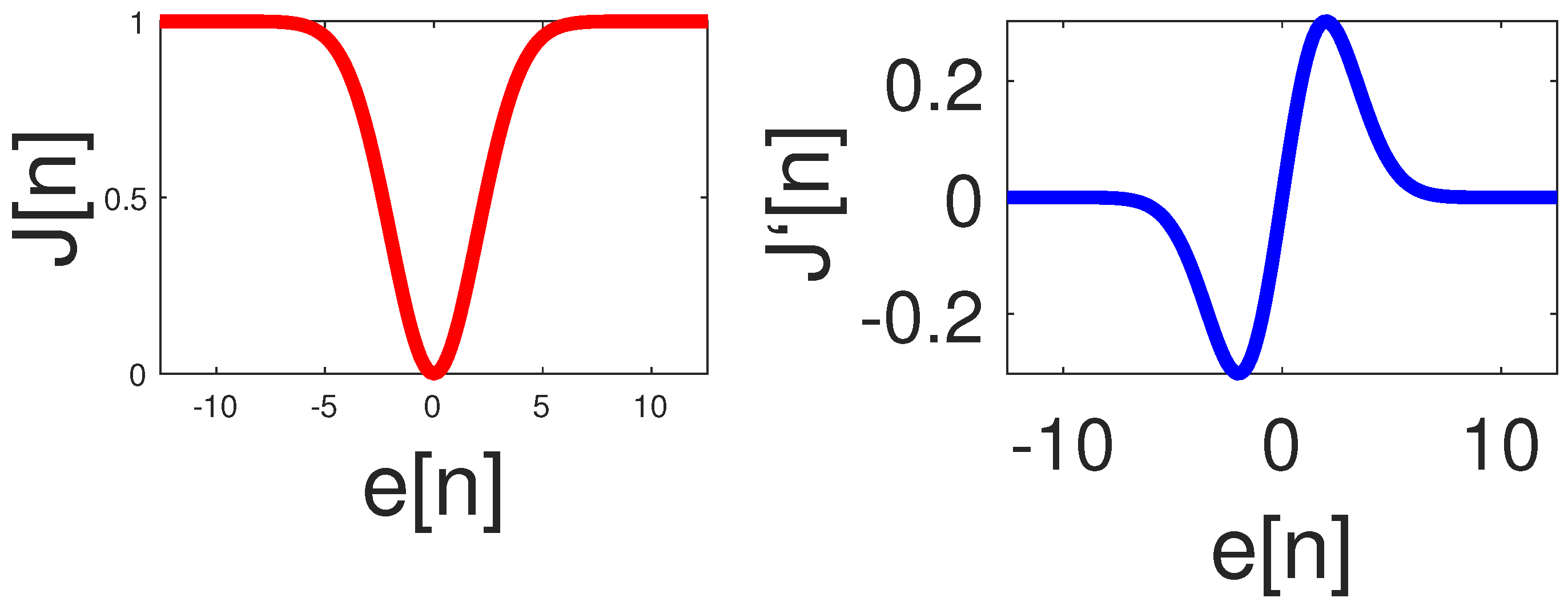
  • We proposed a novel cost function on graph to deal with the impulsive noise environment.
  • The detail analysis of the proposed algorithm is provided.
  • The partial sampling strategy is proposed for WL-G algorithm.
  • WL-G estimation with adaptive graph sampling is also considered to deal with the time-variant graphs.

2. Related Work

First, the papers regarding graph sampling without adaptive strategy are reviewed. Then, we overview graph sampling with adaptive strategy.

2.1. Graph Sampling without Adaptive Strategy

The graph sampling method based on Paley–Wiener was extended and developed in [19,63,64,65,66,67]. For instance, the prerequisite of individual restoration in GSP was provided in [27,66]. The authors also proposed the sampling method based on the Nyquist–Shannon theory. In [27], several greedy sampling methods on graphs were presented and the reconstruction (interpolation) performance of those schemes was also evaluated. Other effective sampling approaches in the graph spectral field were developed in [67].

2.2. Graph Sampling with Adaptive Strategy

Due to the merits of adaptive filter [68,69,70,71], the graph sampling with adaptive strategy has been proposed and developed in [36,72,73,74,75,76]. Specifically, Lorenzo et al. proposed an adaptive method to reconstruct graph signals by exploiting the use of the least mean squares (LMS) strategy [72]. The LMS approach is then extended to the distributed scheme in [74]. To speed up the adaptive estimation, the recursive least square (RLS) method is applied to the reconstruction of signals on graphs [75]. The probabilistic-sampling-based reconstruction approaches are then proposed by using the LMS and RLS strategies in [76]. In [77], to enhance convergence rate of the previous estimation algorithm of graph signals, the authors present two novel adaptive algorithms. First, the extended LMS (ELMS) was proposed, which extends the LMS algorithm via redeveloping the former vectors. To enhance the performance of ELMS, authors present the fast ELMS via using optimization for the gradient MSD. However, these graph sampling methods will suffer from severe performance deterioration when heavy-tailed impulsive noise occurs. The previous references regarding the graph sampling with adaptive strategy have been summarized in Table 1.

3. Background of Graph Signal Processing

Consider an undirected graph G = V , E that is defined by two sets: the set of vertices V = 1 , 2 , , N and the set of weight edges E = a i j i , j V , where a i j > 0 if nodes i and j are connected and a i j = 0 otherwise. Let A be the graph adjacency matrix whose ith entry is a i j representing the edge weight from node i to node j. For undirected graphs, A is symmetric. The degree matrix is a diagonal matrix K , whose i t h diagonal entry is expressed as k i = j = 1 N a i j .
As the most fundamental operator in GSP, the graph Laplacian matrix takes the form L : = K A . Obviously, for undirected graphs, L is also positive semidefinite and symmetric. Therefore, L can be eigendecomposed. Given the eigendecomposition of L as U Λ U T with U = u 1 , u N and Λ = diag λ 1 , λ 2 , , λ N , the ascending-order set of eigenvalues 0 < λ 1 < λ 2 < < λ N denote the graph frequencies.
A signal x : V R N is defined as an N × 1 vector whose ith entry x i represents the vertex value of node i. For graph signal x , the definition of the GFT is given by
s = U T x .
Alternative definitions for the GFT are also available, e.g., via the use of adjacency matrix [10]. We focus on the definition dependent on the Laplacian matrix in this paper.
In many cases, the graph signal is usually band-limited and can be given by
x = U s
where the GFT s is sparse. The support of s is defined as
F = i 1 , , N : s i 0 .
The cardinality of F , i.e., F , leads to the bandwidth of x . We denote D S as the vertex limiting operator:
D S = diag 1 S
where 1 S denotes a vector and S denotes a subset of V , i.e., S V . If i S , the ith element of 1 S becomes 0. For i S , the ith element of 1 S is 1. The band-limiting operator over the set F that satisfies F V is defined as
B F = U Σ F U T
where Σ F denotes a diagonal matrix whose ith diagonal element is zero, if i F , and one otherwise. Note that both matrices D S and B F are idempotent and self-adjoint.

4. Adaptive WL-G Estimation on Graphs

Given a graph signal x o = x o i i = 1 N R N defined over the graph G = V , E , we assume that
Assumption 1. 
(band-limited):  The signal x o is F -bandlimited.
The observed signal is corrupted by the additive noise v n including the background noise η n with covariance matrix C η and the impulsive noise ξ n with covariance matrix C ξ . Therefore, the observed noisy signal has the following form at each time n
y n = D x o + v n = D B x o + D v n
where the D is given by (4). For convenience, we omit the subscript in D S . The covariance matrix of v n can be denoted as C v . The objective of the graph signal reconstruction under consideration is to recover x o . The previous graph signal reconstruction algorithms were developed based on the mean-squared error criterion under the assumption of Gaussian noise. However, the MSE-based approaches are unstable to outliers and thus performs rather poorly under the presence of impulsive noise. To make the recovering process robust against the impulsive noise, we use the cost function based on Welsch loss [61]
f x [ n ] = 1 i = 1 N exp ( e i 2 [ n ] 2 c 2 )
where c denotes a scale parameter that restraints the scale of the quadratic bowl of loss and e i [ n ] is the ith entry of e n with e n = y [ n ] DB x [ n ] . The Welsch loss given by the kernel width verified to be effective in suppressing the impacts of impulsive noise or large outliers. Figure 1 depicts the cost function (7) and its first derivative to demonstrate the robustness of the arctangent function.
An estimate for x o can be obtained by
min x [ n ] E f x [ n ] s.t. B x [ n ] = x [ n ]
This optimization problem is robust against the impulsive noise because the objective function grounded in the Welsch loss has been proven to be insensitive to the impulsive noise [45,78,79]. In contrary to the sign algorithm, which can be derived from the l 1 -norm-based cost function, the Welsch loss is differentiable and mathematically tractable.
A common method to address optimization problem (8) is stochastic steepest-descent method, which is expressed as [62]
x [ n + 1 ] = x [ n ] + μ B D ϕ y n x [ n ]
where μ > 0 denotes the convergence rate, ϕ y n x [ n ] denotes a vector whose ith element is given by ϕ y i n x i [ n ] = exp ( ( y i n x i [ n ] ) 2 2 c 2 ( y i [ n ] x i [ n ] ) and the second equation is relied on the fact that D is an idempotent operator. To satisfy the constraint in (8), the following equation should hold
x [ n + 1 ] = B x [ n + 1 ]
Using (9), we have
B x [ n + 1 ] = B { x [ n ] + μ B D ϕ y n x [ n ] } = B x [ n ] + μ B D ϕ y n x [ n ]
According to (10), to make x [ n + 1 ] = B x [ n + 1 ] hold, x [ n ] should equal to B x [ n ] . Then, we have the following equations
x [ n 1 ] = B x [ n 1 ] , x [ n 2 ] = B x [ n 2 ] , , x [ 1 ] = B x [ 1 ]
To make (12) hold, we have
x [ 0 ] = B x [ 0 ]
In the other words, when the initialization of x [ n ] satisfies x [ 0 ] = B x [ 0 ] , the algorithm (9) satisfies the constraint in (8). The algorithm (9) is referred to as the WL-G algorithm. It is important to note that the properties of the proposed WL-G algorithm is strongly dependent on the sampling matrix D and the band-limiting operator matrix B . Therefore, to optimize the WL-G method, a mean square analysis is presented in the next part to characterize the dependence of the WL-G performance on the choice of sampling matrix D. Using these outcomes, the effective sampling strategies for the WL-G are developed in Section 6. An adaptive graph sampling method is then presented in Section 7.

Computational Complexity

The computational complexity of the LMS, LMP, and WL-G algorithms is provided in Table 2. Compared with LMS, the additional complexity of the WL-G arises from the calculation of function ϕ . Significantly, in spite of growth complexity, the WL-G surpasses the LMS and LMP algorithm.

5. Mean Square Analysis

Rewriting the WL-G algorithm as follows
x i [ n + 1 ] = x i [ n ] + μ j = 1 N b i j d j ϕ y j n x j [ n ] , i = 1 , 2 , , N
We then define the error vector x ˜ [ n ] = x [ n ] x o whose ith entry is x ˜ i [ n ] .
Lemma 1. 
Using (14), the recursion of error vector  x ˜ [ n ]  is given by
x ˜ [ n + 1 ] = I B D D B x ˜ [ n ] + μ B D v n g x [ n ] .
where v n g x [ n ] is defined in Appendix A.
Proof. 
See Appendix A. □
Multiplying both sides of (15) by U T and using (5), we obtain
s ˜ [ n + 1 ] = I Σ U T D D U Σ s ˜ [ n ] + μ Σ U T D v n g x [ n ]
where s ˜ [ n ] = U T x ˜ [ n ] is the GFT of x ˜ [ n ] . We only consider s ^ [ n ] = s ˜ [ n ] , i F R F . The error recursion (16) becomes
s ^ [ n + 1 ] = I Σ U F T D D U F s ^ [ n ] + μ U F T D v n g x [ n ]
where s ^ [ n ] = U F T x ˜ [ n ] .
Using (17), the recursion of E s ^ [ n + 1 ] c 2 can be derived as follows.
Lemma 2. 
E s ^ [ n + 1 ] c 2 can be calculated as
E s ^ [ n + 1 ] c 2 = E s ^ [ n ] Q c 2 + μ 2 vec G T c
where D and Q are given in Appendix B.
Proof. 
See Appendix B. □
According to Lemma 2, we obtain two theorems regarding steady-state mean square deviation (MSD) and convergence stability as follows.
Theorem 1.
Assuming that the data model (6) and Assumption 1 hold, the steady state of the WL-G algorithm is given by
MSD = μ 2 v e c G T I Q 1 v e c ( I ) .
Proof. 
In steady-state, and assuming that the matrix I Q is invertible, from the recursive expression (18), we obtain
lim n E s ^ [ n ] I Q c 2 = μ 2 vec G T c .
Let c = I Q 1 vec ( I ) , we obtain
MSD = μ 2 v e c G T I Q 1 v e c ( I ) .
The theorem is proved. □
Theorem 2.
Assume that Assumption 1 and (6) hold, the WL-G can converge if the step-size μ
0 < μ < 2 λ max U F T D D U F .
Proof. 
Iterating recursion (18) starting from n = 0 , we find that
E s ^ [ n + 1 ] c 2 = E s ^ [ 0 ] Q n + 1 c 2 + μ 2 vec G T i = 0 n Q i c
with initial condition s ^ [ 0 ] . Note Q is stable when I U F T D D U F is stable. Thus, we require 0 < 1 μ λ max U F T D D U F < 1 . After some algebraic manipulations, (22) can be obtained. □

6. Sampling Strategy

According to (18), (19) and (22), the performance of the WL-G algorithm relies on the vertex limiting operator D . Therefore, sampling signals defined on graphs is not only about choosing the number of samples but also about (if possible) having an appropriate strategy to optimally determine where to sample because the sampling locations has a great influence on the performance of the WL-G.
The objective is to determine the optimal sampling set (i.e., the vertex limiting operator D ), which minimizes the value of MSD for sampling strategy. Assuming that the matrix Q can be eigendecomposed by Q = V Π V T , the MSD in (19) can be rewritten as
MSD = μ 2 vec T T I V Π V T 1 vec ( I ) = μ 2 vec T T V I Π 1 V T vec ( I ) = μ 2 i = 1 F 2 p i q i 1 λ i Q .
where q i and p i are the ith terms of the vectors V T vec ( I ) and V T vec ( T ) , respectively. In order to get as a low MSD value as possible, the matrix Q should be selected such that its eigenvalues
λ i Q = 1 μ λ k U F T D D U F 1 μ λ l U F T D D U F
are as far as from 1, where k , l = 1 , 2 , , | F | . In other words, the eigenvalues of the matrix U F T D D U F should differ from 0 as much as possible. As a result, we can use the greedy approximation method to obtain an approximate minimization of (24). The main idea is to iteratively select the samples from the graph that maximize the pseudodeterminant of the matrix U F T D D U F , denoted by Det U F T D D U F . Using the greedy method results in the sampling strategy (called the greedy determinant–maximization method) as given in Table 3. Since the computational steps of the greedy determinant–maximization sampling strategy have high computation complexity, it is desirable to reduce the computational complexity while at the same not significantly compromising the reconstruction performance. Motivated by the partial method in [80,81], we propose the partial greedy approach as summarized in Table 4, where p is the partial probability and randit ( 1 , ( 1 p ) N , [ 1 , N ] ) denotes ( 1 p ) N random integer sets between 1 and N.
In Table 5, we provide the framework of proposed WL-G estimation algorithm. N in Table 5 denotes the iteration number.

7. Wl-G Estimation with AGS
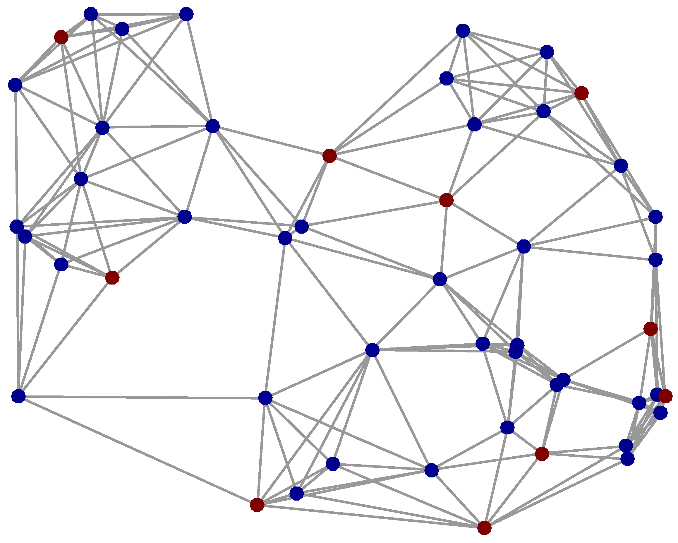
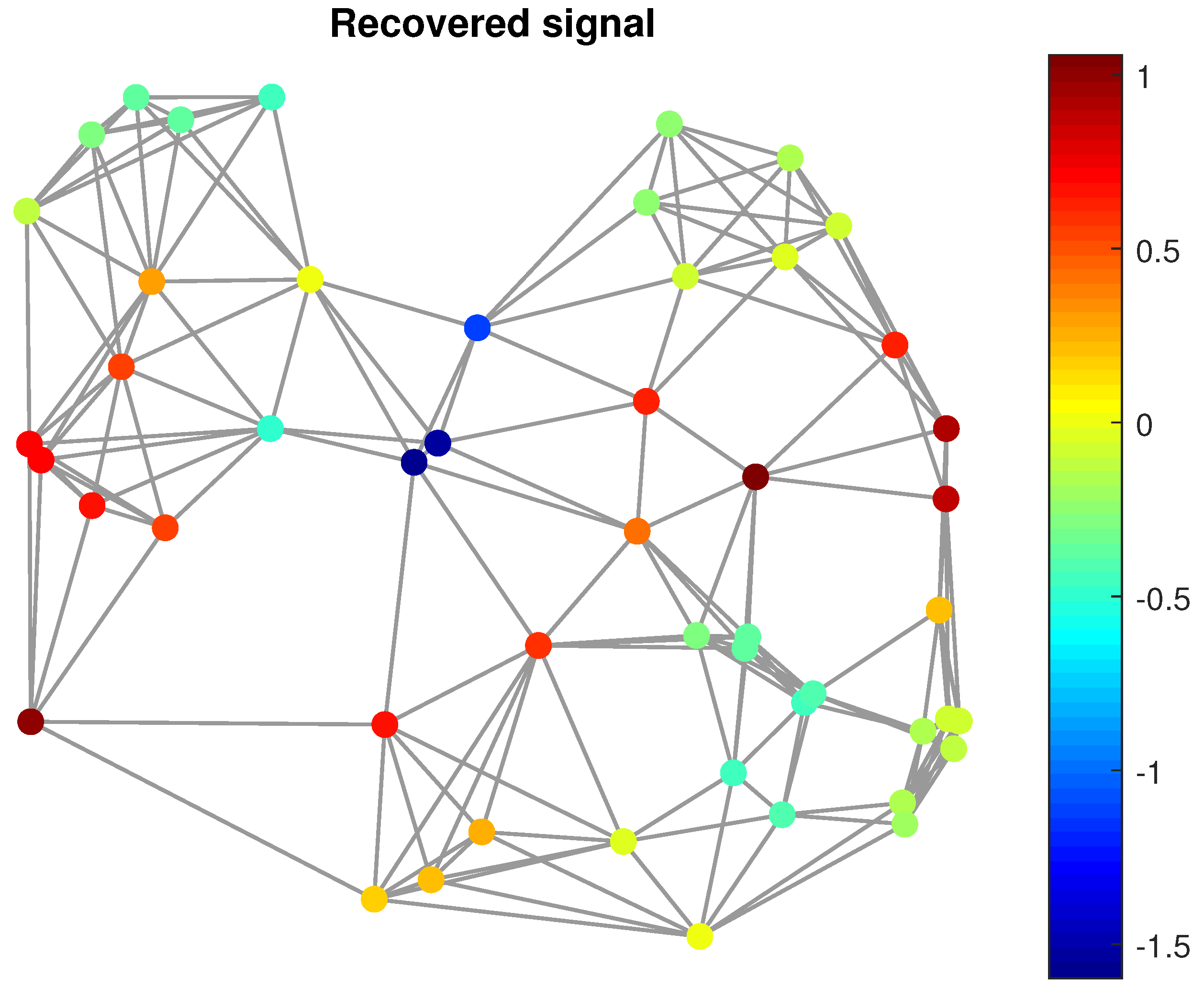
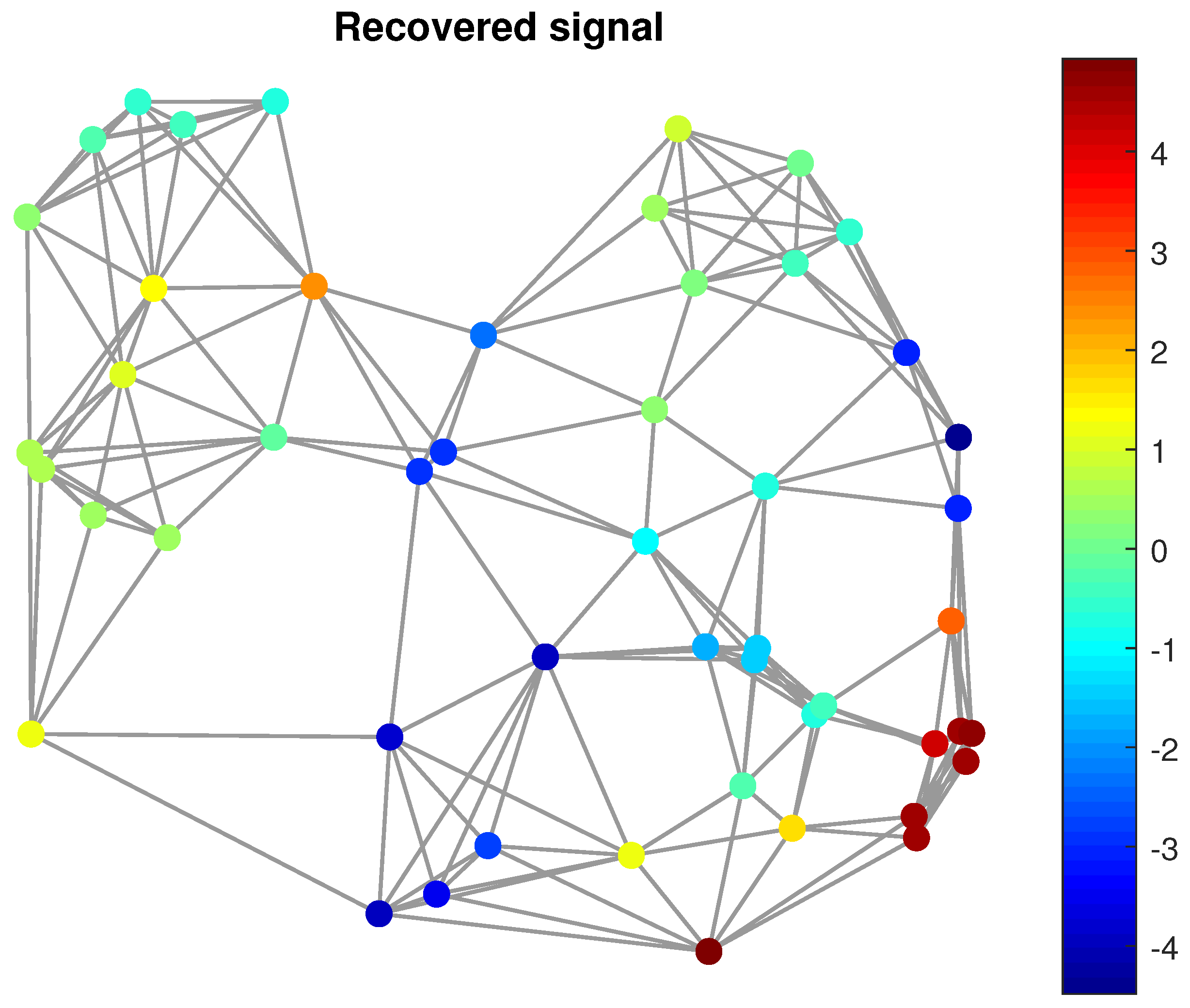
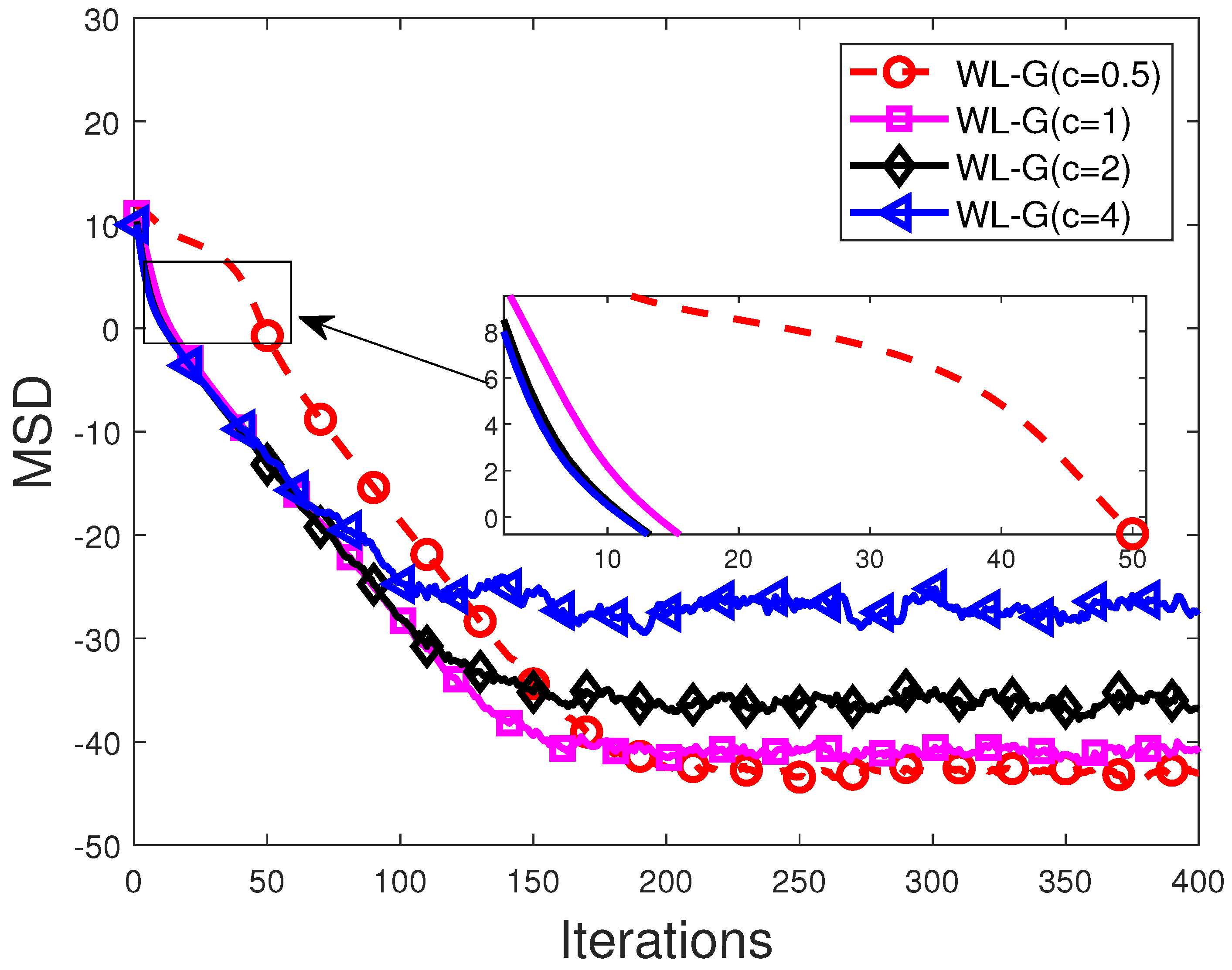
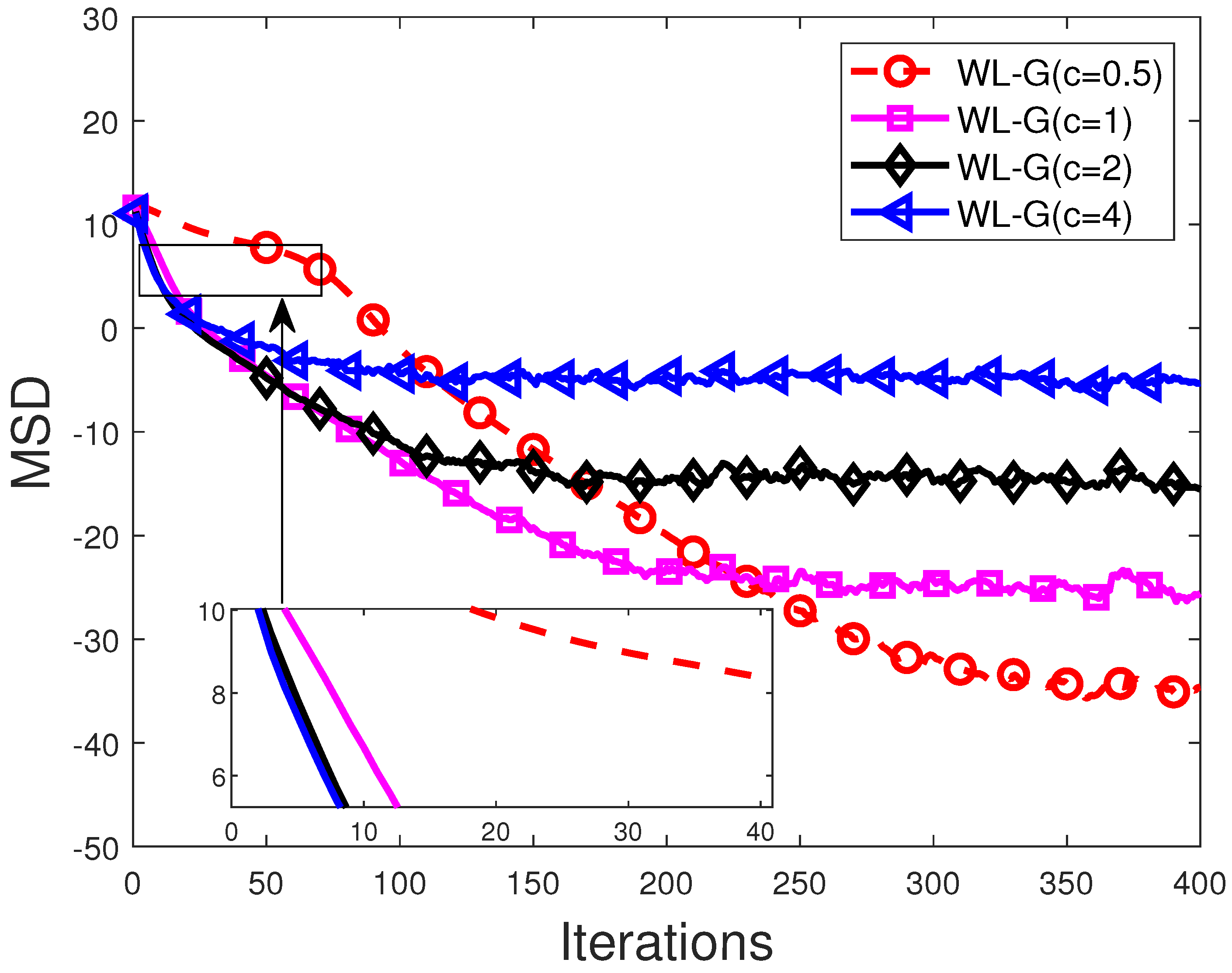
The band-limiting operator B is assumed in (9) to be known in advance. However, since the graph may vary over time, the prior knowledge of B is sometimes unrealistic in certain applications. To overcome the lack of prior knowledge of B , we present an AGS technique for the WL-G algorithm.
Using (1), the graph signal observation model can be rewritten as
y n = D U s o + D v n .
As a result, estimating x o is equivalent to estimating s o . Motivating by the fact that the support identification for s o is acutely associated with the set of sampling, the optimal problem (8) could be recast as
min s , D E f s + λ g ( s )
where g ( · ) is a l 0 norm or l 1 norm, and λ denotes a constant that regulates the sparsity level of s . The minimization problem (26) is a nonconvex program; thus, it is generally challenging to be solved. The ISTA [82] is adopted to solve (26). Provided D [ n ] , s is updated through the improved ISTA algorithm as
s [ n + 1 ] = T γ ( s [ n ] + μ f s s [ n ] ) = T γ ( s [ n ] + μ U T D [ n ] ϕ y n U s [ n ] )
where T γ is a thresholding function, μ denotes a step-size. Here, the thresholding function is selected as a hard threshold given by
T γ ( s m ) = s m s m > γ 0 s m < γ .
where T γ ( s m ) is the mth element of the thresholding function T γ ( s ) .

8. Simulation

This part carries out simulation examples to demonstrate the advantages of the proposed algorithm on graphs and verify the correctness of the performance analysis. A graph signal with 50 nodes is considered. The graph is depicted in Figure 2.

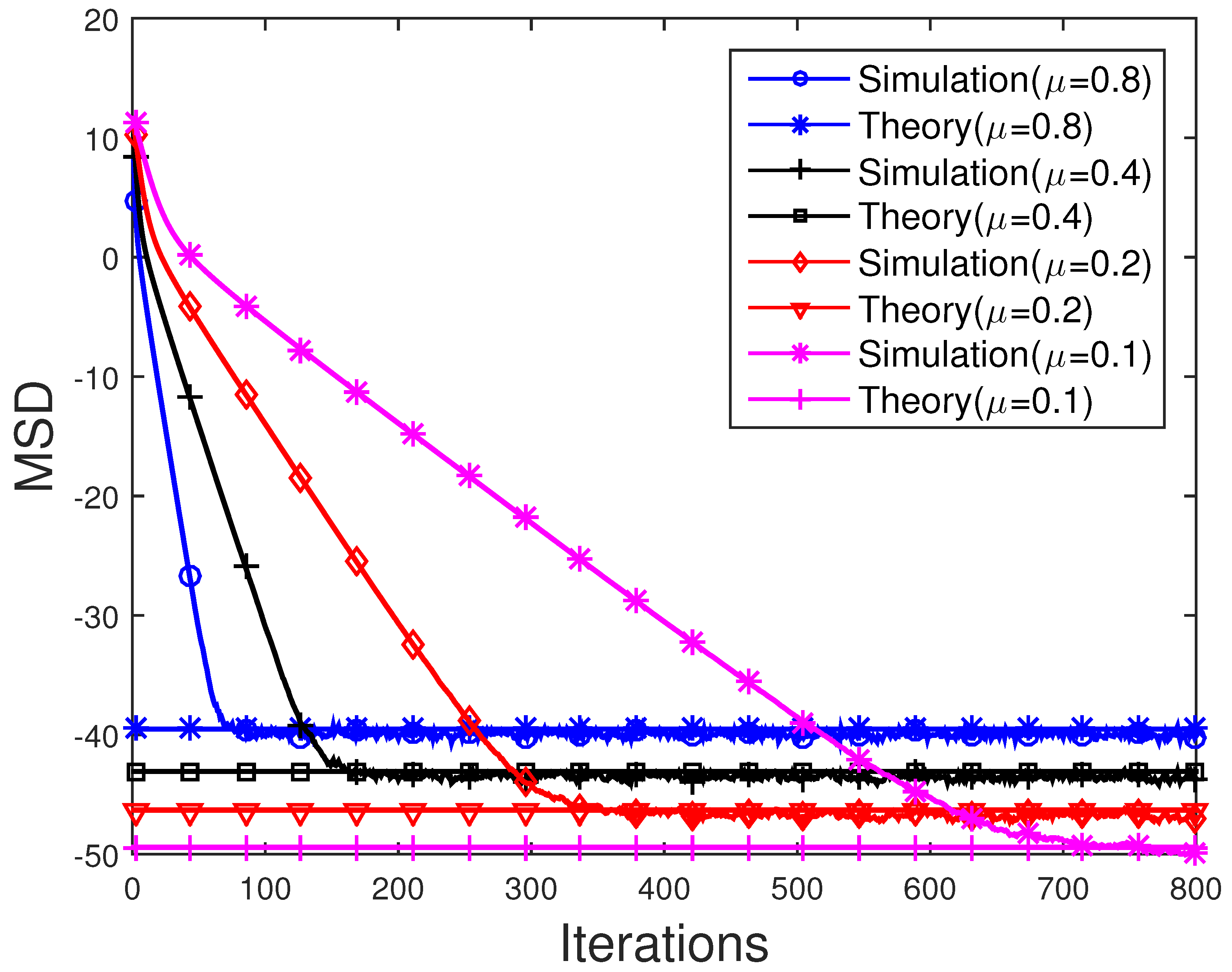
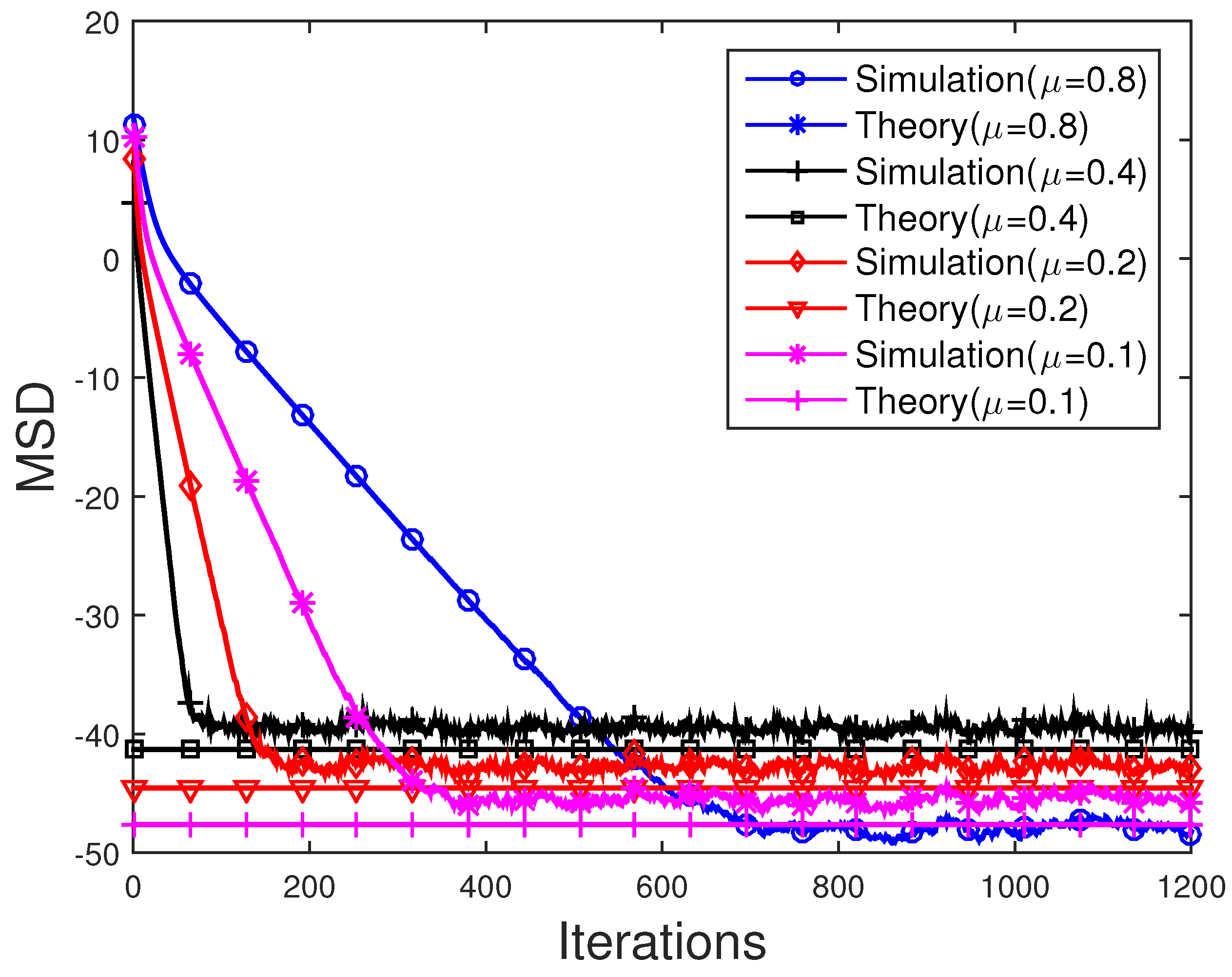
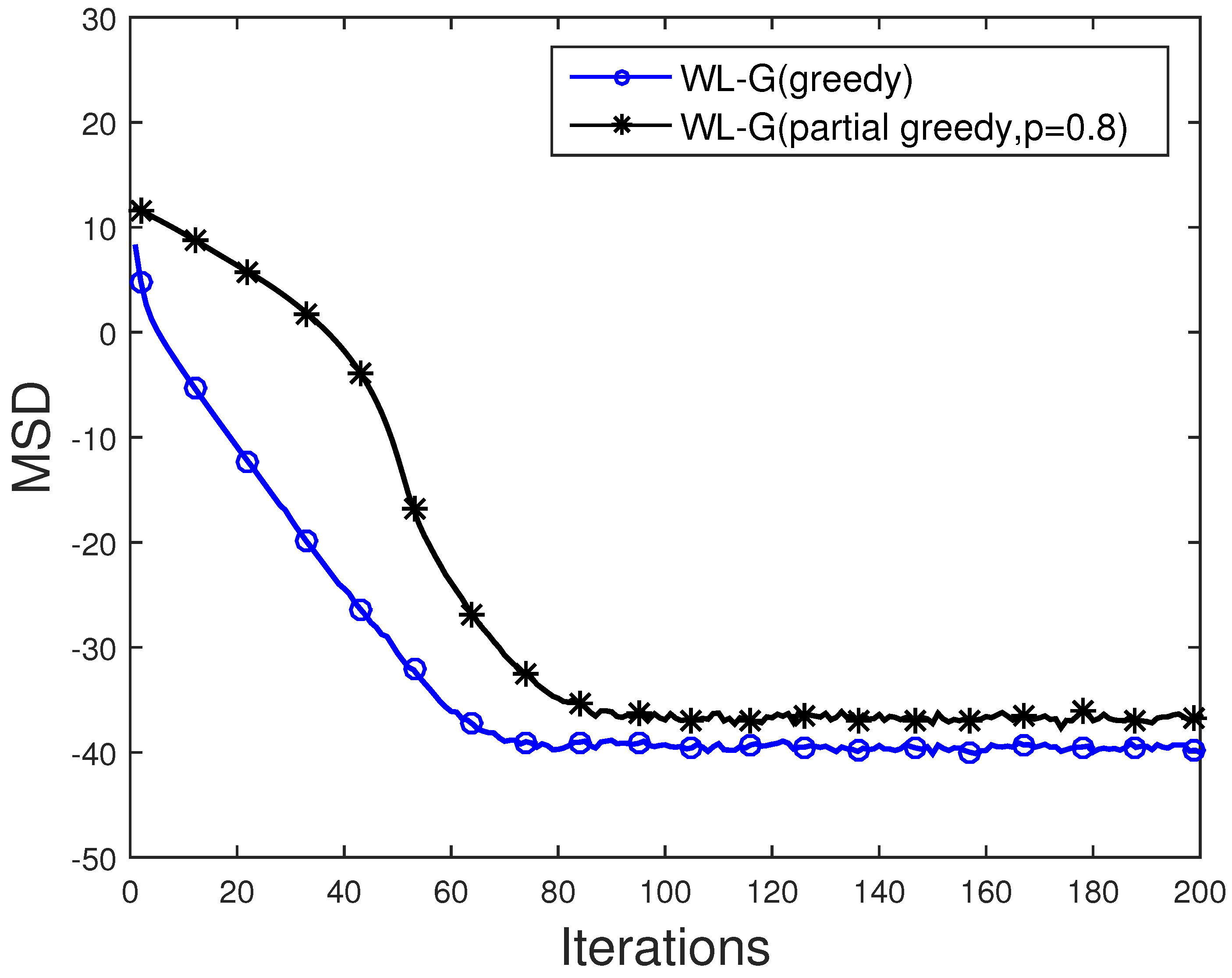
8.1. On the Theoretical Results

We now verify the precision of the mean square analytical theory provided in Theorem 1 by comparing the analytical MSD values with the MSD obtained via simulations for both the cases of nonimpulsive noise and impulsive noise. | F | is set to 10.
Example 1. 
(No impulsive Noise):In this scenario, the observation noise only contains the background noise. The background noise η [ n ] is the zero-mean Gaussian process with diagonal covariance matrix,
C η = c η , 1 2 c η , 2 2 c η , N 2
where c η , i 2 is generated uniformly randomly between 0 and 0.01. Figure 3 shows the simulated MSD of the WL-G compared with the theoretical MSD value given by Theorem 1 for various values of the step sizes μ = 0.001 , 0.003 , 0.006 , 0.008 . Here, S is set to 10. The steady-state MSD of WL-G gained from the experiments closely match the analytical MSD value given by Theorem 1. This thus confirms the correctness of the mean square analysis given by Theorem 1. In addition, it is observed that, although providing a higher learning rate (convergence rate) of the WL-G algorithm, a larger μ results in an inferior property. In contrast, a smaller value of step size results in a better MSD performance of the WL-G algorithm but with a slower learning rate.
Example 2. 
(Impulsive Noise):This example considers the case of impulsive noise where the impulsive noise ξ [ n ] is generated from the Bernoulli–Gaussian (BG) process, which is often used in the performance analysis. By denoting ξ i n as the ith element of ξ n , we have ξ i n = b i n g i n , where b i n is a Bernoulli process whose probabilities are expressed by P b i n = 1 = P i , and g i n is a zero-mean white Gaussian process with variance κ c η , i 2 . Note that p r , i stands for the probability of occurrence of impulsive noise sample. In the simulation, the probability p r , i is set to 0.05, and the constant κ is set to 10,000. In addition to the impulsive noise ξ [ n ] , the background noise η [ n ] is generated in the same manner as in Example 1. Figure 4 compares the transient behavior of the MSD of the WL-G algorithm with the theoretical steady-state MSD value given in Theorem 1 for the step sizes of μ = 0.0008 , 0.001 , 0.003 , 0.006 . A similar observation as in Example 1 is made here, where the theoretical steady-state MSD value derived in Theorem 1 closely agrees with the simulated steady-state MSD. This once again verifies the correctness of Theorem 1.

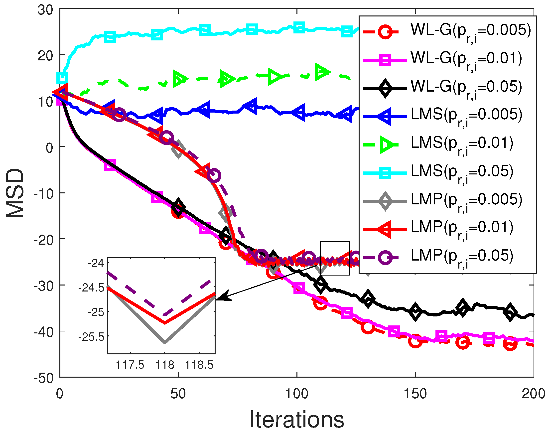
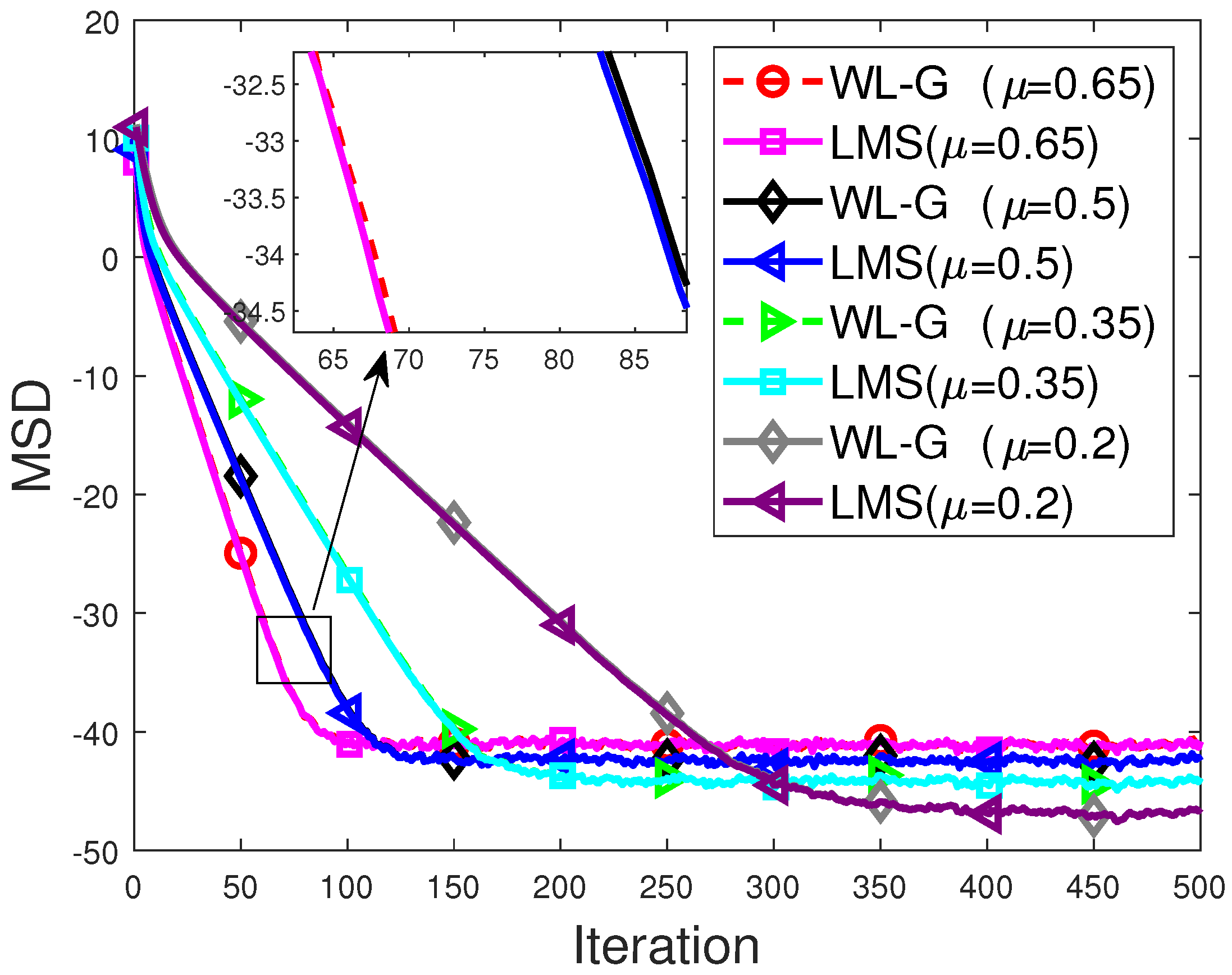
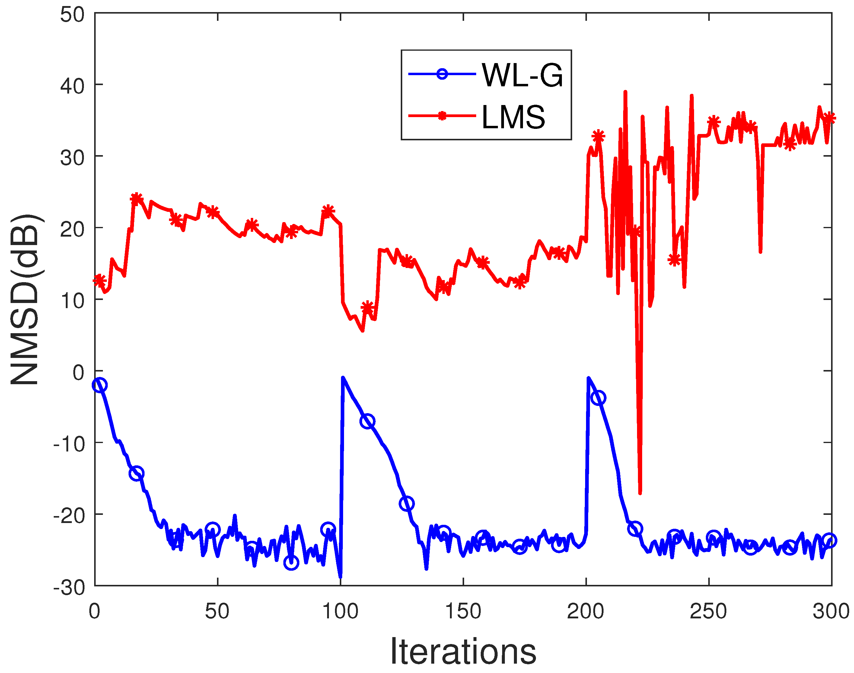
8.2. On the Performance of The WL-G Algorithm

Example 3. 
(Effect of Cardinality S ):This example examines how the behavior of the WL-G algorithm is affected by the number of samples in the observation set S . Figure 5 plots the transient MSD of the WL-G algorithm for | S | = 10 , 20 , 30 , and 40. Here, the simulation setup is the same as in Example 2 except that the step size is set to 0.06 . We can see from Figure 5 that, as expected, growing the samples improve the convergence speed.
Example 4. 
(WL-G Versus LMS):In this example, the behavior of WL-G algorithm is compared with those of the LMS algorithm [72] and the LMP algorithm on graph. Here, the cardinality S is set to 10. The probabilities P i are set to 0.05, 0.01, and 0.005. Other parameters remain the same as those in Example 3.
Figure 6 compares the WL-G, LMP, and LMS on graph in the impulsive noise background. It is observed that the LMS algorithms yields a poor MSD performance due to the impulsive noise. It is as expected as the LMS algorithm is in virtue of MSE criterion which is unstable to outliers. In contrast, the WL-G and the LMP algorithm on graph can effectively cope with the impulsive noise by producing a much more reliable MSD performance.
The MSD curves of the WL-G and LMS algorithm in the Guassian noise are depicted in Figure 7. As can be seen from Figure 7, we obtain that the WL-G algorithm exhibits nearly same performance as the LMS algorithm.
Figure 8, Figure 9 and Figure 10 shows the measured graph signal and the reconstructed graph signals obtained by the LMS and WL-G algorithms. The WL-G algorithm is observed to produce a reconstructed signal that is almost identical to the ground-truth signal in Figure 2. On the other hand, the LMS algorithm results in an unsatisfactory reconstructed signal where the signal values at most of the nodes are far different from the corresponding true values. These observations demonstrate one more time the performance advantages of the proposed WL-G algorithm over the LMS.
Example 5. 
(Effect of scale parameter c ):This example examines how the performance of the WL-G algorithm is affected by the scale parameter c. Figure 8 and Figure 9 depict the MSD curves of the WL-G algorithm with different scale parameters c under impulsive noise, where p r , i are set to 0.05 and 0.5 in Figure 11 and Figure 12, respectively. Smaller c leads to smaller steady-state error but lower convergence rate. Therefore, we can select a suitable value for c according to the specific requirement.
Example 6. 
(WL-G (greedy) Versus WL-G (partial greedy)):We conduct the simulation to test the partial greedy approach, where p is set to 0.8 . The simulated result is depicted in Figure 13. From the results of the simulation, we can determine that the algorithm in Table 4 has the similar performance to the algorithm in Table 3.

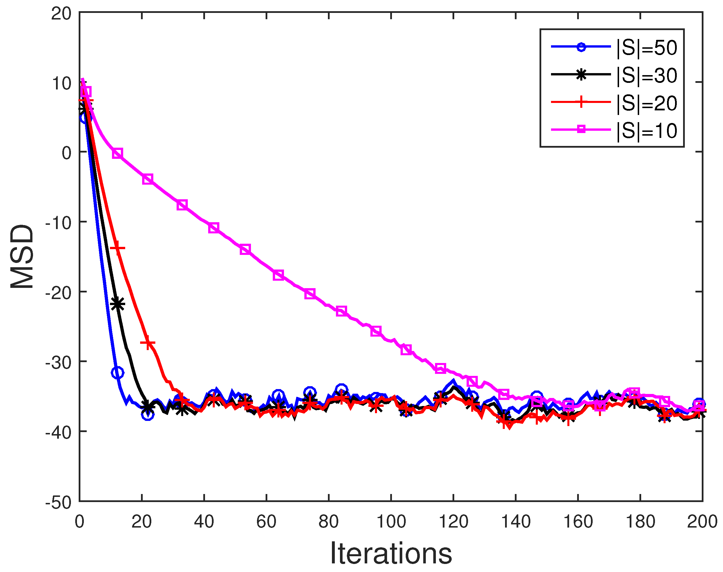
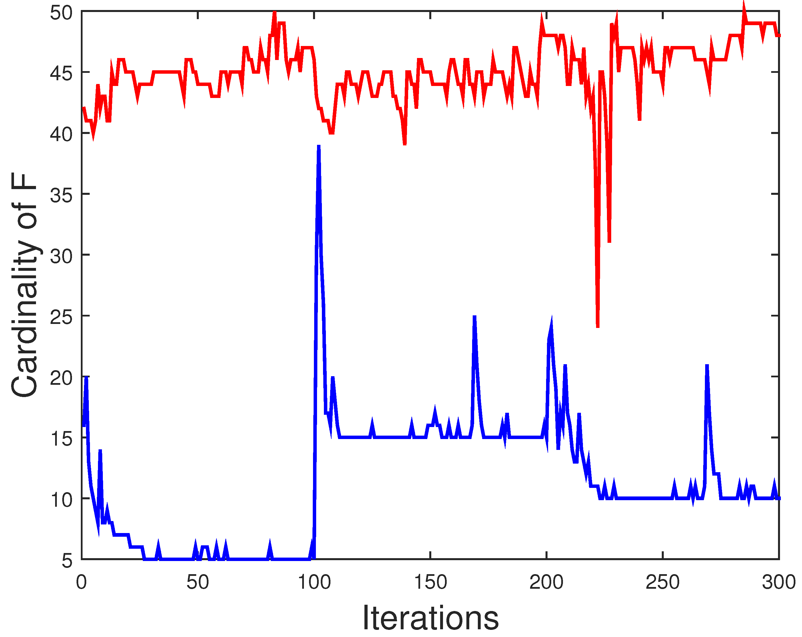
8.3. On the Performance of WL-G Algorithm with Adaptive Graph Sampling

In this section, we present a performance evaluation for the proposed WL-G algorithm with adaptive graph sampling. A time-varying graph signal with N = 50 nodes is considered, where the spectral content of the signal switches between the first 5, 15, and 10 eigenvectors. The graph topology is the same as in Figure 3. The elements of the GFT s o inside the support are set to 1. The observation noise consists of both background noise and impulsive noise. The background noise has covariance matrix C η = c η 2 I where c η 2 = 2 × 10 4 . The impulsive noise follows the Bernoulli–Gaussian (BG) process as described in Section 8.1, where the probability p r , i is set to 0.05 and the constant κ associated with the noise level is set to κ = 1000 . The step size μ , the sparsity parameter λ , and the hard threshold value γ are set to 0.9, 0.056, and 0.05, respectively. The normalized mean-square deviation (NMSD), i.e., NMSD [ n ] = | | s [ n ] s 0 | | 2 / | | s 0 | | 2 , is adopted as the measurement to evaluate the performance of the proposed algorithm.
Figure 14 shows the performance of the WL-G in comparison with that of the LMS algorithm with adaptive sampling. Similar to other simulation examples, the proposed WL-G algorithm significantly outperforms the LMS algorithm. The LMS algorithms produces an unreliable NMSD performance. In contrast, the WL-G algorithm is capable of effectively tracking the time-varying scenarios. Specifically, the sudden increases in the NMSD performance of the WL-G algorithm correspond to the changes in the spectral content of the signal. However, by adapting the sampling set, the WL-G algorithm is able to quickly converge to the steady state conditions. Figure 15 depicts the F curves of WL-G with adaptive sampling in comparison to LMS with adaptive sampling.
Figure 16, Figure 17 and Figure 18 report the samples chosen by the proposed WL-G algorithm at iterations n = 86 , n = 150 , and n = 279 .

9. Discussion

9.1. Discussion about Adaptive WL-G Estimation on Graphs

Comparing the Equation (9) with the LMS algorithm in [72], we obtain that the update equation of the WL-G algorithm contains just an extra scaling factor exp ( ( y i n x i [ n ] ) 2 2 c 2 ) The outlier rejection property of theWelsch loss can be reflected from this factor [45]. Therefore, if the desired graph signal has impulsive characteristics or strong outliers, the WL-G is more stable than LMS algorithm in [72]. It is worth noting that the computational complexity of the WL-G algorithm is slightly more than that of the LMS algorithm. To implement the WL-G algorithm compared with LMS, we need only a few extra multiplications and additions.

9.1.1. Discussion about WL-G Estimation with AGS

The WL-G estimation on graphs in Table 5 supposes complement awareness of the support. Nevertheless, this assumption is fantastic in the practice, because the signal, the signal model, and the graph topology might be time-variant. The WL-G estimation with AGS is proposed. The signal support is tracked and estimated via the WL-G estimation, which is also fit to the AGS strategy.

9.1.2. Discussion about Simulation Results

Figure 3 and Figure 4 verify the precision of the mean square analytical theory provided in Theorem 1. From Figure 3 and Figure 4, we can determine that notional outcomes computed by (19) can fit fully with the simulated outcomes. Figure 6 verifies advantages belongs to WL-G algorithm on graph under the impulsive noise environment. From Figure 6, we get the WL-G can effectively cope with the impulsive noise by producing a much more reliable MSD performance. Figure 14 verifies the merits of WL-G algorithm with adaptive graph sampling. The proposed algorithm can get lower MSD and faster convergence rate. In summary, Figure 3 and Figure 4 in simulation section validate the precision of theory analysis in Theorem 1 while Figure 6 and Figure 14 verifies the advantages of proposed algorithms.

10. Conclusions

We propose the WL-G algorithm for adaptive graph signal reconstruction with impulsive noise in this work. Different to existing LMS methods, which are based on the least-squares criterion, the proposed WL-G leverages the use of Welsch loss to formulate its cost function. The framework of the WL-G algorithm is given in Table 5. The proposed algorithm can leverage the graph signal’s basal framework to recover signals from partial observations with impulsive noises under a band-limited supposition. The relationship between the sampling strategy and the performance of the WL-G algorithm was revealed via the theoretical analysis on the performance of the WL-G algorithm. Effective sampling strategies were then developed relied on analysis. An adaptive graph sampling technique was developed and used in conjunction with the WL-G algorithm to determine the support in the GFD while allowing the graph sampling strategy to be adapted in an online manner. Extensive simulation is carried out to verify the analysis and merits of the proposed algorithms. Specifically, Figure 3 and Figure 4 show that our theoretical analysis is correct, since theoretical results match well with the simulated results. Figure 6 show that the WL-G is sturdy against the impulsive interference. Figure 14 shows the proposed WL-G algorithm with the adaptive sampling strategy.

Author Contributions

Conceptualization, W.W. and Q.S.; methodology, Q.S.; software, W.W.; validation, Q.S.; investigation, Q.S.; resources, Q.S.; data curation, W.W.; writing—original draft preparation, W.W.; writing—review and editing, W.W.; visualization, Q.S.; supervision, Q.S.; project administration, Q.S.; funding acquisition, W.W. All authors have read and agreed to the published version of the manuscript.

Funding

This research was funded by National Natural Science Foundation of China: 62101215.

Data Availability Statement

Not applicable.

Conflicts of Interest

The authors declare no conflict of interest.

Appendix A. Proof of the Lemma 1

Using (6) and the definition of error vector, the term ϕ y j n x j [ n ] in (14) can be expressed as
ϕ y j n x j [ n ] = ϕ x o j + v j n x j [ n ] = ϕ x ˜ j [ n ] + v j n .
where v j [ n ] is the the ith entry of v [ n ] . We approximate ϕ x ˜ j [ n ] + v j n using a first-order Taylor series approximation of the function ϕ x around x ˜ j [ n ] = 0 ,
ϕ x ˜ j [ n ] + v j n ϕ v j n x ˜ j [ n ] ϕ v j n
The expectation of the term ϕ x ˜ j [ n ] + v j n is expressed as
E ϕ x ˜ j [ n ] + v j n = E x ˜ j [ n ] E ϕ v j n = E x ˜ j [ n ] ϕ ¯ v j
where ϕ ¯ v j = E ϕ v j n . Let g ^ j , n x ˜ j [ n ] = ϕ x ˜ j [ n ] + v j n ϕ v j n x ˜ j [ n ] ϕ v j n , Equation (14) can be rewritten as
x i [ n + 1 ] = x i [ n ] + μ j = 1 N b i j d j g ^ j , n x j [ n ] .
Using (A2), the update term g ^ j , n in term of x F [ n 1 ] can be approximated by
g ^ j , n x ϕ v j n + x o j x ϕ v j n .
where F [ n 1 ] denotes filtration generated by the past history of iterations x ˜ j [ m ] for m n 1 and all j. For adequately big n, we have
E g ^ j , n x F [ n 1 ] = ϕ ¯ v j x o j x g j x .
In other words, there exists a deterministic function such that, for all x in the filtration F [ n 1 ] , it holds that
E g ^ j , n x F [ n 1 ] = g j x .
Taking the gradient of the function g j x , we obtain
D j = x g j x = ϕ ¯ v j .
The noise incurred by stochastic approximation for each node j and any x F [ n 1 ] , i.e., the update noise is defined as
v j , n g x g ^ j , n x g j x .
Using (A9) and (A4) implies
x i [ n + 1 ] = x i [ n ] + μ j = 1 N b i j d j g j x j [ n ] + v j , n g x j [ n ] .
Subtracting x o i from (A10) yields
x ˜ i [ n + 1 ] = x ˜ i [ n ] + μ j = 1 N b i j d j g j x j [ n ] + v j , n g x j [ n ] .
Using some basic algebra manipulations, we have
g j x j [ n ] = g j x o j 0 1 x g j x o j t x j [ n ] d t x ˜ j [ n ] = D j x ˜ j [ n ] .
where the second equation holds due to (A8) and the fact that g j x o j = 0 . Using (A12), the error recursion (A11) becomes
x ˜ i [ n + 1 ] = x ˜ i [ n ] + μ j = 1 N b i j d j D j x ˜ j [ n ] + v j , n g x j [ n ] .
Using the following definitions,
v n g x [ n ] col v 1 , n g x 1 [ n ] , v 2 , n g x 2 [ n ] , , v N , n g x N [ n ] ,
D = diag D 1 , D 2 , , D N ,
Equation (A13) implies
x ˜ [ n + 1 ] = I B D D B x ˜ [ n ] + μ B D v n g x [ n ] .

Appendix B. Proof of the Lemma 2

At the steady state, the update noise vector v n g x [ n ] can be approximated by
v n g x [ n ] v n g x o g ^ n x o g x o g ^ n x o ϕ v n
where g ^ n x o is the vector whose jth term is g ^ j , n x o j and h v n is the vector whose jth term is h v j n . Thus, the covanriance of ϕ v n is denoted by
C v g = E { ϕ v n ϕ v T n }
Evaluating the weighted norm of s ^ [ n ] in (17), we obtain:
E s ^ [ n + 1 ] Ψ 2 = E s ^ [ n ] Ψ 2 + μ 2 Tr Ψ U F T D C v g D U F
where Ψ is any Hermitian positive-definite matrix, which can be chosen freely. Tr · represents the trace operator, and
Ψ = I Σ U F T D D U F Ψ I Σ U F T D D U F .
Vectorizing matrices Ψ and Ψ by c = vec ( Ψ ) and c = vec ( Ψ ) , it can be verified that:
c = Q c
where the matrix Q is given by:
Q = I U F T D D U F Ψ I U F T D D U F .
Equation (A19) can then be expressed as:
E s ^ [ n + 1 ] c 2 = E s ^ [ n ] Q c 2 + μ 2 vec G T c
where
G = U F T D C v g D U F .

References

  1. Yang, G.; Yang, L.; Yang, Z.; Huang, C. Efficient Node Selection Strategy for Sampling Bandlimited Signals on Graphs. IEEE Trans. Signal Process. 2021, 69, 5815–5829. [Google Scholar] [CrossRef]
  2. Tanaka, Y.; Eldar, Y.C. Generalized Sampling on Graphs With Subspace and Smoothness Priors. IEEE Trans. Signal Process. 2020, 68, 2272–2286. [Google Scholar] [CrossRef] [Green Version]
  3. Ruiz, L.; Chamon, L.; Ribeiro, A.R. Graphon Signal Processing. IEEE Trans. Signal Process. 2021, 69, 4961–4976. [Google Scholar] [CrossRef]
  4. Romero, D.; Mollaebrahim, S.; Beferull-Lozano, B.; Asensio-Marco, C. Fast Graph Filters for Decentralized Subspace Projection. IEEE Trans. Signal Process. 2021, 69, 150–164. [Google Scholar] [CrossRef]
  5. Ramakrishna, R.; Scaglione, A. Grid-Graph Signal Processing (Grid-GSP): A Graph Signal Processing Framework for the Power Grid. IEEE Trans. Signal Process. 2021, 69, 2725–2739. [Google Scholar] [CrossRef]
  6. Polyzos, K.D.; Lu, Q.; Giannakis, G.B. Ensemble Gaussian processes for online learning over graphs with adaptivity and scalability. IEEE Trans. Signal Process. 2021, 26, 1. [Google Scholar] [CrossRef]
  7. Morency, M.W.; Leus, G. Graphon Filters: Graph Signal Processing in the Limit. IEEE Trans. Signal Process. 2021, 69, 1740–1754. [Google Scholar] [CrossRef]
  8. Meyer, F.; Williams, J.L. Scalable Detection and Tracking of Geometric Extended Objects. IEEE Trans. Signal Process. 2021, 69, 6283–6298. [Google Scholar] [CrossRef]
  9. Ibrahim, S.; Fu, X. Mixed Membership Graph Clustering via Systematic Edge Query. IEEE Trans. Signal Process. 2021, 69, 5189–5205. [Google Scholar] [CrossRef]
  10. Sandryhaila, A.; Moura, J.M.F. Discrete signal processing on graphs. IEEE Trans. Signal Process. 2013, 61, 1644–1656. [Google Scholar] [CrossRef] [Green Version]
  11. Ortega, A.; Frossard, P.; Kovačević, J.; Moura, J.M.F.; Vandergheynst, P. Graph signal processing: Overview, challenges, and applications. Proc. IEEE 2018, 106, 808–828. [Google Scholar] [CrossRef] [Green Version]
  12. Shuman, D.I.; Narang, S.K.; Frossard, P.; Ortega, A.; Vandergheynst, P. The emerging field of signal processing on graphs: Extending high-dimensional data analysis to networks and other irregular domains. arXiv 2012, arXiv:1211.0053. [Google Scholar] [CrossRef] [Green Version]
  13. Wang, Y.; Sun, Y.; Liu, Z.; Sarma, S.E.; Bronstein, M.M.; Solomon, J.M. Dynamic graph cnn for learning on point clouds. arXiv 2018, arXiv:1801.07829. [Google Scholar] [CrossRef] [Green Version]
  14. Rustamov, R.; Guibas, L.J. Wavelets on graphs via deep learning. Adv. Neural Inf. Process. Syst. 2013, 26, 998–1006. [Google Scholar]
  15. Mao, X.; Qiu, K.; Li, T.; Gu, Y. Spatio-temporal signal recovery based on low rank and differential smoothness. IEEE Trans. Signal Process. 2018, 66, 6281–6296. [Google Scholar] [CrossRef]
  16. Mao, X.; Gu, Y.; Yin, W. Walk Proximal Gradient: An Energy-Efficient Algorithm for Consensus Optimization. IEEE Internet Things J. 2018, 6, 2048–2060. [Google Scholar] [CrossRef]
  17. Mao, X.; Yuan, K.; Hu, Y.; Gu, Y.; Sayed, A.H.; Yin, W. Walkman: A communication-efficient random-walk algorithm for decentralized optimization. IEEE Trans. Signal Process. 2020, 68, 2513–2528. [Google Scholar] [CrossRef]
  18. Qiu, K.; Mao, X.; Shen, X.; Wang, X.; Li, T.; Gu, Y. Time-varying graph signal reconstruction. IEEE J. Sel. Top. Signal Process. 2017, 11, 870–883. [Google Scholar] [CrossRef]
  19. Marques, A.G.; Segarra, S.; Leus, G.; Ribeiro, A. Sampling of Graph Signals With Successive Local Aggregations. IEEE Trans. Signal Process. 2016, 64, 1832–1843. [Google Scholar] [CrossRef]
  20. Sandryhaila, A.; Moura, J.M. Discrete signal processing on graphs: Frequency analysis. IEEE Trans. Signal Process. 2014, 62, 3042–3054. [Google Scholar] [CrossRef] [Green Version]
  21. Segarra, S.; Marques, A.G.; Mateos, G.; Ribeiro, A. Network topology inference from spectral templates. IEEE Trans. Signal Inf. Process. Netw. 2017, 3, 467–483. [Google Scholar] [CrossRef]
  22. Shahid, N.; Perraudin, N.; Kalofolias, V.; Puy, G.; Vandergheynst, P. Fast robust PCA on graphs. IEEE J. Sel. Top. Signal Process. 2016, 10, 740–756. [Google Scholar] [CrossRef] [Green Version]
  23. Chen, S.; Cerda, F.; Rizzo, P.; Bielak, J.; Garrett, J.H.; Kovačević, J. Semi-supervised multiresolution classification using adaptive graph filtering with application to indirect bridge structural health monitoring. IEEE Trans. Signal Process. 2014, 62, 2879–2893. [Google Scholar] [CrossRef]
  24. Loukas, A.; Simonetto, A.; Leus, G. Distributed autoregressive moving average graph filters. IEEE Signal Process. Lett. 2015, 22, 1931–1935. [Google Scholar] [CrossRef] [Green Version]
  25. Teke, O.; Vaidyanathan, P.P. Extending Classical Multirate Signal Processing Theory to Graphs-Part II: M-Channel Filter Banks. IEEE Trans. Signal Process. 2017, 65, 423–437. [Google Scholar] [CrossRef]
  26. Sardellitti, S.; Barbarossa, S.; Di Lorenzo, P. On the graph Fourier transform for directed graphs. IEEE J. Sel. Top. Signal Process. 2017, 11, 796–811. [Google Scholar] [CrossRef] [Green Version]
  27. Chamon, L.F.O.; Ribeiro, A. Greedy sampling of graph signals. IEEE Trans. Signal Process. 2018, 66, 34–47. [Google Scholar] [CrossRef]
  28. Chen, S.; Varma, R.; Sandryhaila, A.; Kovačević, J. Discrete Signal Processing on Graphs: Sampling Theory. IEEE Trans. Signal Process. 2015, 63, 6510–6523. [Google Scholar] [CrossRef] [Green Version]
  29. Pesenson, I. Sampling in Paley-Wiener spaces on combinatorial graphs. Trans. Am. Math. Soc. 2008, 360, 5603–5627. [Google Scholar] [CrossRef] [Green Version]
  30. Mengüç, E.C. Design of quaternion-valued second-order Volterra adaptive filters for nonlinear 3-D and 4-D signals. Signal Process. 2020, 174, 107619. [Google Scholar] [CrossRef]
  31. Yang, L.; Liu, J.; Zhang, Q.; Yan, R.; Chen, X. Frequency domain spline adaptive filters. Signal Process. 2020, 177, 107752. [Google Scholar] [CrossRef]
  32. Zhou, S.; Zhao, H. Statistics variable kernel width for maximum correntropy criterion algorithm. Signal Process. 2020, 176, 107589. [Google Scholar] [CrossRef]
  33. Shen, M.; Xiong, K.; Wang, S. Multikernel adaptive filtering based on random features approximation. Signal Process. 2020, 176, 107712. [Google Scholar] [CrossRef]
  34. Wang, W.; Zhao, H. A novel block-sparse proportionate NLMS algorithm based on the l2,0 norm. Signal Process. 2020, 176, 107671. [Google Scholar] [CrossRef]
  35. Nguyen, N.H.; Doğançay, K.; Wang, W. Adaptive estimation and sparse sampling for graph signals in alpha-stable noise. Digit. Signal Process. 2020, 105, 102782. [Google Scholar] [CrossRef]
  36. Di Lorenzo, P.; Banelli, P.; Barbarossa, S.; Sardellitti, S. Distributed adaptive learning of signals defined over graphs. In Proceedings of the 2016 50th Asilomar Conference on Signals, Systems and Computers, Pacific Grove, CA, USA, 6–9 November 2016; pp. 527–531. [Google Scholar]
  37. Sayed, A.H. Adaptive Filters; John Wiley & Sons: Hoboken, NJ, USA, 2011. [Google Scholar]
  38. Al-Sayed, S.; Zoubir, A.M.; Sayed, A.H. Robust adaptation in impulsive noise. IEEE Trans. Signal Process. 2016, 64, 2851–2865. [Google Scholar] [CrossRef]
  39. Al-Sayed, S.; Zoubir, A.M.; Sayed, A.H. Robust distributed estimation by networked agents. IEEE Trans. Signal Process. 2017, 65, 3909–3921. [Google Scholar] [CrossRef]
  40. Nguyen, N.H.; Doğançay, K. Improved Weighted Instrumental Variable Estimator for Doppler-Bearing Source Localization in Heavy Noise. In Proceedings of the 2018 IEEE International Conference on Acoustics, Speech and Signal Processing (ICASSP), Calgary, AB, Canada, 15–20 April 2018; pp. 3529–3533. [Google Scholar]
  41. Georgiou, P.G.; Tsakalides, P.; Kyriakakis, C. Alpha-stable modeling of noise and robust time-delay estimation in the presence of impulsive noise. IEEE Trans. Multimed. 1999, 1, 291–301. [Google Scholar] [CrossRef] [Green Version]
  42. Pascal, F.; Forster, P.; Ovarlez, J.P.; Larzabal, P. Performance analysis of covariance matrix estimates in impulsive noise. IEEE Trans. Signal Process. 2008, 56, 2206–2217. [Google Scholar] [CrossRef] [Green Version]
  43. Wang, W.; Zhao, H.; Doğançay, K.; Yu, Y.; Lu, L.; Zheng, Z. Robust adaptive filtering algorithm based on maximum correntropy criteria for censored regression. Signal Process. 2019, 160, 88–98. [Google Scholar] [CrossRef]
  44. Liu, W.; Pokharel, P.P.; Príncipe, J.C. Correntropy: Properties and applications in non-Gaussian signal processing. IEEE Trans. Signal Process. 2007, 55, 5286–5298. [Google Scholar] [CrossRef]
  45. Chen, B.; Xing, L.; Zhao, H.; Zheng, N.; Prı, J.C. Generalized correntropy for robust adaptive filtering. IEEE Trans. Signal Process. 2016, 64, 3376–3387. [Google Scholar] [CrossRef] [Green Version]
  46. Shin, J.; Yoo, J.; Park, P. Variable step-size sign subband adaptive filter. IEEE Signal Process. Lett. 2013, 20, 173–176. [Google Scholar] [CrossRef]
  47. Zou, Y.; Chan, S.C.; Ng, T.S. Least mean M-estimate algorithms for robust adaptive filtering in impulse noise. IEEE Trans. Circuits Syst. II Analog Digit. Signal Process. 2000, 47, 1564–1569. [Google Scholar]
  48. Chan, S.C.; Zou, Y.X. A recursive least M-estimate algorithm for robust adaptive filtering in impulsive noise: Fast algorithm and convergence performance analysis. IEEE Trans. Signal Process. 2004, 52, 975–991. [Google Scholar] [CrossRef]
  49. Jung, S.M.; Park, P. Normalised least-mean-square algorithm for adaptive filtering of impulsive measurement noises and noisy inputs. Electron. Lett. 2013, 49, 1270–1272. [Google Scholar] [CrossRef]
  50. Chan, S.C.; Wen, Y.; Ho, K.L. A robust past algorithm for subspace tracking in impulsive noise. IEEE Trans. Signal Process. 2006, 54, 105–116. [Google Scholar] [CrossRef] [Green Version]
  51. Nguyen, N.H.; Dogancay, K. An Iteratively Reweighted Instrumental-Variable Estimator for Robust 3D AOA Localization in Impulsive Noise. IEEE Trans. Signal Process. 2019, 67, 4795–4808. [Google Scholar] [CrossRef]
  52. Chen, B.; Xing, L.; Liang, J.; Zheng, N.; Príncipe, J.C. Steady-State Mean-Square Error Analysis for Adaptive Filtering under the Maximum Correntropy Criterion. IEEE Signal Process. Lett. 2014, 21, 880–884. [Google Scholar] [CrossRef]
  53. Singh, A.; Principe, J.C. Using correntropy as a cost function in linear adaptive filters. In Proceedings of the 2009 International Joint Conference on Neural Networks, Atlanta, GA, USA, 14–19 June 2009; pp. 2950–2955. [Google Scholar]
  54. Chen, B.; Liu, X.; Zhao, H.; Principe, J.C. Maximum correntropy Kalman filter. Automatica 2017, 76, 70–77. [Google Scholar] [CrossRef] [Green Version]
  55. Giannakis, G.B.; Kekatos, V.; Gatsis, N.; Kim, S.J.; Zhu, H.; Wollenberg, B.F. Monitoring and optimization for power grids: A signal processing perspective. IEEE Signal Process. Mag. 2013, 30, 107–128. [Google Scholar] [CrossRef] [Green Version]
  56. Drayer, E.; Routtenberg, T. Detection of false data injection attacks in smart grids based on graph signal processing. IEEE Syst. J. 2019, 14, 1886–1896. [Google Scholar] [CrossRef] [Green Version]
  57. Drayer, E.; Routtenberg, T. Detection of false data injection attacks in power systems with graph fourier transform. In Proceedings of the 2018 IEEE Global Conference on Signal and Information Processing (GlobalSIP), Anaheim, CA, USA, 26–28 November 2018; pp. 890–894. [Google Scholar]
  58. Grotas, S.; Yakoby, Y.; Gera, I.; Routtenberg, T. Power Systems Topology and State Estimation by Graph Blind Source Separation. IEEE Trans. Signal Process. 2019, 67, 2036–2051. [Google Scholar] [CrossRef] [Green Version]
  59. Singer, A.; Shkolnisky, Y. Three-dimensional structure determination from common lines in cryo-EM by eigenvectors and semidefinite programming. SIAM J. Imaging Sci. 2011, 4, 543–572. [Google Scholar] [CrossRef] [PubMed]
  60. Giridhar, A.; Kumar, P.R. Distributed clock synchronization over wireless networks: Algorithms and analysis. In Proceedings of the 45th IEEE Conference on Decision and Control, San Diego, CA, USA, 13–15 December 2006; pp. 4915–4920. [Google Scholar]
  61. Dennis, J.E., Jr.; Welsch, R.E. Techniques for nonlinear least squares and robust regression. Commun. Stat.-Simul. Comput. 1978, 7, 345–359. [Google Scholar] [CrossRef]
  62. Haykin, S.S. Adaptive Filter Theory; Pearson Education: Chennai, India, 2005. [Google Scholar]
  63. Wang, X.; Liu, P.; Gu, Y. Local-set-based graph signal reconstruction. IEEE Trans. Signal Process. 2015, 63, 2432–2444. [Google Scholar] [CrossRef]
  64. Chen, S.; Varma, R.; Singh, A.; Kovačević, J. Signal recovery on graphs: Fundamental limits of sampling strategies. IEEE Trans. Signal Inf. Process. Netw. 2016, 2, 539–554. [Google Scholar] [CrossRef] [Green Version]
  65. Tsitsvero, M.; Barbarossa, S.; Di Lorenzo, P. Signals on graphs: Uncertainty principle and sampling. IEEE Trans. Signal Process. 2016, 64, 4845–4860. [Google Scholar] [CrossRef] [Green Version]
  66. Anis, A.; Gadde, A.; Ortega, A. Towards a sampling theorem for signals on arbitrary graphs. In Proceedings of the 2014 IEEE International Conference on Acoustics, Speech and Signal Processing (ICASSP), Florence, Italy, 4–9 May 2014; pp. 3864–3868. [Google Scholar]
  67. Tanaka, Y. Spectral domain sampling of graph signals. IEEE Trans. Signal Process. 2018, 66, 3752–3767. [Google Scholar] [CrossRef] [Green Version]
  68. Shin, J.; Kim, J.; Kim, T.K.; Yoo, J. p-Norm-like Affine Projection Sign Algorithm for Sparse System to Ensure Robustness against Impulsive Noise. Symmetry 2021, 13, 1916. [Google Scholar] [CrossRef]
  69. Dogariu, L.M.; Stanciu, C.L.; Elisei-Iliescu, C.; Paleologu, C.; Benesty, J.; Ciochină, S. Tensor-Based Adaptive Filtering Algorithms. Symmetry 2021, 13, 481. [Google Scholar] [CrossRef]
  70. Li, G.; Zhang, H.; Zhao, J. Modified Combined-Step-Size Affine Projection Sign Algorithms for Robust Adaptive Filtering in Impulsive Interference Environments. Symmetry 2020, 12, 385. [Google Scholar] [CrossRef] [Green Version]
  71. Guo, Y.; Li, J.; Li, Y. Diffusion Correntropy Subband Adaptive Filtering (SAF) Algorithm over Distributed Smart Dust Networks. Symmetry 2019, 11, 1335. [Google Scholar] [CrossRef] [Green Version]
  72. Di Lorenzo, P.; Barbarossa, S.; Banelli, P.; Sardellitti, S. Adaptive least mean squares estimation of graph signals. IEEE Trans. Signal Inf. Process. Netw. 2016, 2, 555–568. [Google Scholar] [CrossRef] [Green Version]
  73. Di Lorenzo, P.; Ceci, E. Online Recovery of Time-varying Signals Defined over Dynamic Graphs. In Proceedings of the 2018 26th European Signal Processing Conference (EUSIPCO), Rome, Italy, 3–7 September 2018; pp. 131–135. [Google Scholar]
  74. Di Lorenzo, P.; Banelli, P.; Barbarossa, S.; Sardellitti, S. Distributed adaptive learning of graph signals. IEEE Trans. Signal Process. 2017, 65, 4193–4208. [Google Scholar] [CrossRef] [Green Version]
  75. Di Lorenzo, P.; Isufi, E.; Banelli, P.; Barbarossa, S.; Leus, G. Distributed recursive least squares strategies for adaptive reconstruction of graph signals. In Proceedings of the 2017 25th European Signal Processing Conference (EUSIPCO), Kos Island, Greece, 28 August–2 September 2017; pp. 2289–2293. [Google Scholar]
  76. Di Lorenzo, P.; Banelli, P.; Isufi, E.; Barbarossa, S.; Leus, G. Adaptive graph signal processing: Algorithms and optimal sampling strategies. IEEE Trans. Signal Process. 2018, 66, 3584–3598. [Google Scholar] [CrossRef] [Green Version]
  77. Ahmadi, M.J.; Arablouei, R.; Abdolee, R. Efficient Estimation of Graph Signals With Adaptive Sampling. IEEE Trans. Signal Process. 2020, 68, 3808–3823. [Google Scholar] [CrossRef]
  78. Shao, T.; Zheng, Y.R.; Benesty, J. An affine projection sign algorithm robust against impulsive interferences. IEEE Signal Process. Lett. 2010, 17, 327–330. [Google Scholar] [CrossRef]
  79. Yoo, J.; Shin, J.; Park, P. A band-dependent variable step-size sign subband adaptive filter. Signal Process. 2014, 104, 407–411. [Google Scholar] [CrossRef]
  80. Dogancay, K. Partial-Update Adaptive Signal Processing: Design Analysis and Implementation; Academic Press: Orlando, FL, USA, 2008. [Google Scholar]
  81. Arablouei, R.; Werner, S.; Huang, Y.F.; Doğançay, K. Distributed least mean-square estimation with partial diffusion. IEEE Trans. Signal Process. 2014, 62, 472–484. [Google Scholar] [CrossRef]
  82. Beck, A.; Teboulle, M. A fast iterative shrinkage-thresholding algorithm for linear inverse problems. SIAM J. Imaging Sci. 2009, 2, 183–202. [Google Scholar] [CrossRef] [Green Version]
Figure 1. Cost function based on Welsch loss and its derivative.
Symmetry 14 00426 g001
Figure 2. Graph topology and graph signal.
Symmetry 14 00426 g002
Figure 3. Transient behavior of the MSD of the WL-G algorithm in comparison with the theoretical steady-state MSD value given in Theorem 1 for the case of nonimpulsive noise.
Symmetry 14 00426 g003
Figure 4. Transient behavior of the MSD of the WL-G algorithm in comparison with the theoretical steady-state MSD value given in Theorem 1 for the case of impulsive noise.
Symmetry 14 00426 g004
Figure 5. Transient MSD for different S .
Symmetry 14 00426 g005
Figure 6. Performance comparison between the WL-G, LMP, and LMS algorithms with impulsive noise.
Symmetry 14 00426 g006
Figure 7. Performance comparison between the WL-G and LMS algorithms without impulsive noise.
Symmetry 14 00426 g007
Figure 8. Measured signals ( n = 126 ).
Symmetry 14 00426 g008
Figure 9. Reconstructed signals obtained by the WL-G algorithm.
Symmetry 14 00426 g009
Figure 10. Reconstructed signals obtained by the LMS algorithms.
Symmetry 14 00426 g010
Figure 11. MSD curves of WL-G for different values of c with p r , i = 0.05 .
Symmetry 14 00426 g011
Figure 12. MSD curves of WL-G for different values of c with p r , i = 0.5 .
Symmetry 14 00426 g012
Figure 13. MSD performance of the WL-G (greedy) and WL-G (partial greedy) algorithms.
Symmetry 14 00426 g013
Figure 14. MSD performance of WL-G with adaptive sampling in comparison to LMS with adaptive sampling.
Symmetry 14 00426 g014
Figure 15. F curves of WL-G with adaptive sampling in comparison to LMS with adaptive sampling (Red: LMS; Blue: WL-G).
Symmetry 14 00426 g015
Figure 16. Optimal sampling at iteration n = 86 (depicted as brown nodes).
Symmetry 14 00426 g016
Figure 17. Optimal sampling at iteration n = 150 (depicted as brown nodes).
Symmetry 14 00426 g017
Figure 18. Optimal sampling at iteration n = 279 (depicted as brown nodes).
Symmetry 14 00426 g018
Table 1. Graph sampling with adaptive strategy.
The LiteratureAlgorithm
[72]LMS on graph
[74]Distributed LMS on graph
[75]RLS on graph
[76]probabilistic LMS and RLS on graph
[77]ELMS and FELMS on graph
Table 2. Graph sampling with adaptive strategy.
AlgorithmMultiplicationsAdditionsp-NormExponent
LMS on graph N ( N + 1 ) 2 N 2 --
LMP on graph N ( N + 1 ) 2 N 2 N-
WL-G 2 N 2 2 N 2 + 2 N -N
Table 3. Maximizing Det U F T D D U F .
Inputdata:M
Outputdata: S
Initialization: S
Function:
while S < M
s = arg max j Det U F T D S j D U F
S = S s
end
Table 4. Partial greedy determinant–maximization sampling strategy.
Inputdata:M
Outputdata: S
Initialization: S
Function:
for i = 1 : M
K i = { 1 , , N }
T i = randit ( 1 , ( 1 p ) N , [ 1 , N ] )
s = arg max j K i \ T i Det U F T D S j D U F +
S = S s
end
Table 5. Framework of proposed WL-G algorithm.
Problem: Recovering the band-limited graph signal x o from partial observations y n = D B x o + D v n with impulsive noise.
Inputdata:M, y n , N
Outputdata: x [ n ]
Initialization: S , x [ 0 ]
Function:
while S < M
s = arg max j Det U F T D S j D U F
S = S s
end
Using S to calculate D
while n < N
x [ n + 1 ] = x [ n ] + μ B D ϕ y n x [ n ]
end
Publisher’s Note: MDPI stays neutral with regard to jurisdictional claims in published maps and institutional affiliations.

