Abstract
The performance of artificial nanomotors is still far behind nature-made biomolecular motors. A mechanistic disparity between the two categories exists: artificial motors often rely on a single mechanism to rectify directional motion, but biomotors integrate multiple mechanisms for better performance. This study proposes a design for a motor-track system and shows that by introducing asymmetric compound foot-track interactions, both selective foot detachment and biased foot-track binding arise from the mechanics of the system. The two mechanisms are naturally integrated to promote the motility of the motor towards being unidirectional, while each mechanism alone only achieves 50% directional fidelity at most. Based on a reported theory, the optimization of the motor is conducted via maximizing the directional fidelity. Along the optimization, the directional fidelity of the motor is raised by parameters that concentrate more energy on driving selective-foot detachment and biased binding, which in turn promotes work production due to the two energies converting to work via a load attached. However, the speed of the motor can drop significantly after the optimization because of energetic competition between speed and directional fidelity, which causes a speed-directional fidelity tradeoff. As a case study, these results test thermodynamic correlation between the performances of a motor and suggest that directional fidelity is an important quantity for motor optimization.
1. Introduction
A frontier of nano science and technology is developing nanomotors that utilize local energy supply but generate long-range directional motion [1,2,3]. A particularly research interest is fabricating bio-mimicking nanomotors [4,5,6,7,8,9,10,11,12,13] that move along linear tracks for transportation, force generation or perform other functions. Applications of the nanomotors have been demonstrated, including cargo sorting and assembly [14,15], landscape navigation [16,17] and chemical synthesis and catalysis [18,19,20]. Despite the progresses, performances of the artificial nanomotors are magnitudes behind bio-molecular motors.
An important reason for the advanced performance of biomotors is the integration of multiple mechanisms for direction rectification. For example, cellular motor kinesin [21] is a bipedal motor that walks along the filamentous track of the cytoskeleton in a hand-over-hand fashion. Although the two feet of kinesin are identical and equally capable of catalyzing fuel reaction (ATP hydrolysis) for driving, kinesin as a whole achieves both preferential detachment of the rear foot (fuel-gating mechanism) and forward binding of the detached foot (zippering mechanism). As a result, the two identical feet avoid random stepping but cooperate with each other for unidirectional walking. A recent theory [22] shows that a bipedal nanomotor rectifying directional motion singly by selective detachment or forward binding are generally subject to a directional-fidelity limit, namely 50% probability for forward steps at most. The limit can be broken by the integration of the two mechanisms together. Moreover, the mechanistic integration also relates to the optimality of a nanomotor. A thermodynamic study [23] suggests that the directional fidelity of a motor is correlated with other performances of the motor, i.e., work production, energy efficiency and speed, while the value of directional fidelity mainly depends on the actual energy used for driving the selective foot detachment and biased binding. The result suggests that the optimization of a nanomotor can be conducted by maximizing the motor’s directional fidelity. Some predictions of the study have been verified by experimental data from kinesin [23] and F1-ATPase [24], which display advanced performances shown by many experiments. Since optimized artificial nanomotors are desirable for real applications, the mechanistic integration as well as the quantity of directional fidelity may provide a potential path for realizing advanced artificial nanomotors.
However, in the aim of studying upper limit of performances, the reported studies [22,23] use simplified kinetic pictures for treating working processes of nanomotors, in which foot detachment and binding are independent of each other, and the overall working of a motor follows a single cycle. In reality, the movement of a nanomotor is governed by mechanics, which correlates the foot detachment with the binding, and the dynamics of a nanomotor usually includes multiple pathways, which are entangled with each other. Under realistic conditions, how to design both a biased foot detachment and binding inside a single motor and avoid negative restrictions between them is not clear, and the possibility of optimizing the working of a motor that may go through different pathways is not known. To demonstrate the possibilities is meaningful for developing advanced artificial nanomotors.
This study proposes a general design of a motor-track system that integrates both selective foot detachment and biased binding. The two mechanisms arise from intrinsic mechanics of the motor via an asymmetric compound foot–track interaction. The two mechanisms are unified in a single working cycle and coherently add each other beyond the directional fidelity limit of 50%. Based on the reported study [23], the optimization of the motor is conducted via scanning parameters of the motor for maximizing the directional fidelity. The optimization shows that the directional fidelity is enlarged by parameters that concentrate more energy for driving selective foot detachment and biased binding. The two energies meanwhile contribute to output work, and thus the optimization promotes work production. However, energetic competition between directional fidelity and speed occurs when the fidelity is extremely close to 100%, which displays a tradeoff between the two performances. A detailed model and results are shown below.
2. Theoretical Model and Methods
2.1. The Motor-Track System
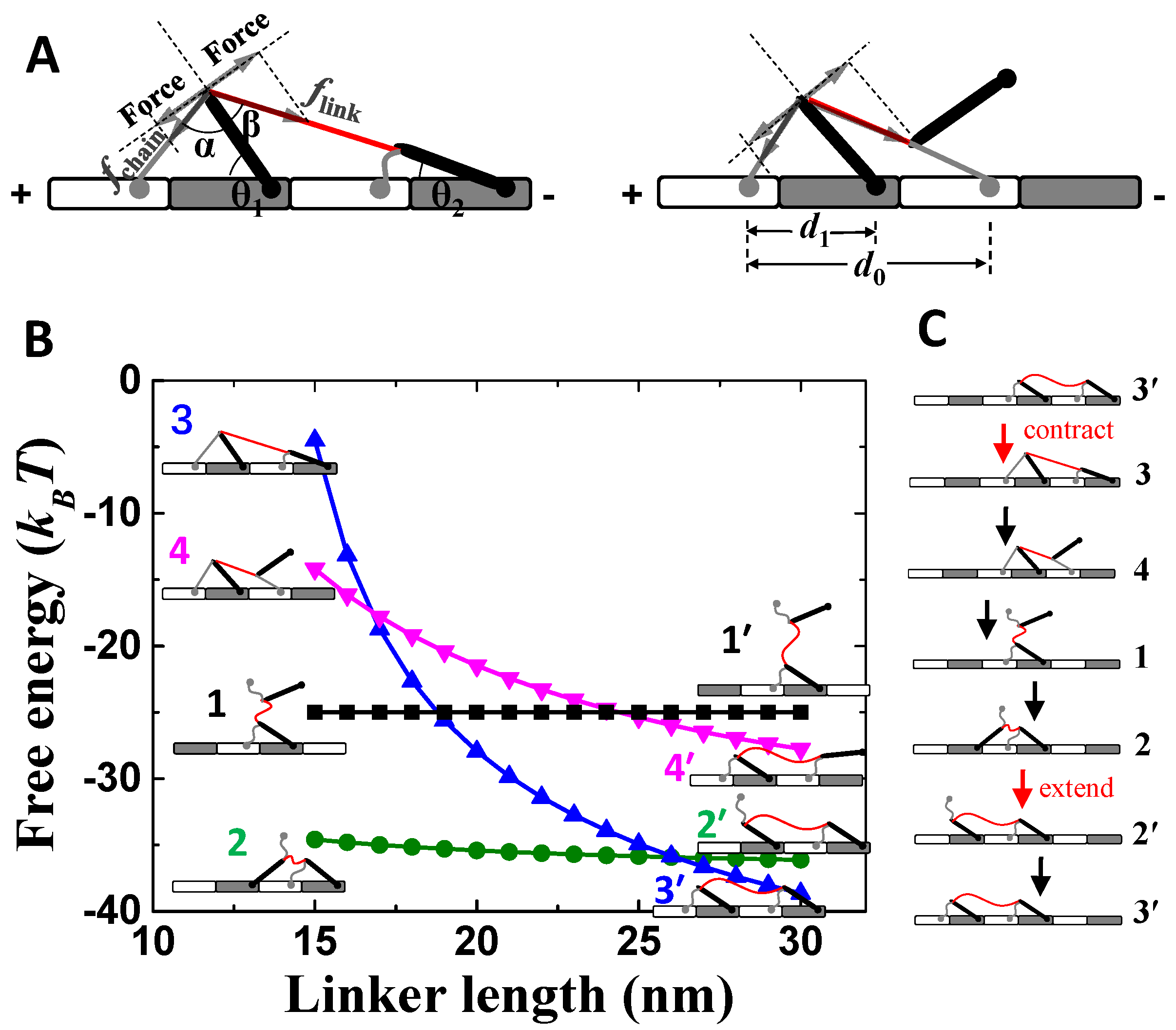
The motor comprises of two identical compound feet and a soft linker for connecting the two feet (Figure 1A). Each compound foot contains a soft and a rigid component, which refer to “foot chain” (gray line in Figure 1A) and “foot bone” (black rod Figure 1A), respectively. The foot chain and foot bone connect with the linker at one end, while the other ends can bind to the track (Figure 1A). The track is assembled by two basic units (the white and gray bricks in Figure 1A), which contain different binding sites for the foot chain and foot bone, respectively. The binding sites are periodically positioned along the track, which is quantified by lattice constants d0 and d1 (Figure 1A). The track is polar because the two basic units are chemically different. Thus, a plus and a minus end are defined as shown in Figure 1A.

Figure 1.
Mechanical analysis of the motor-track binding states. (A) The red line and gray line are the linker and foot chain of the motor, and the thick black line is the foot bone of the motor. The white and gray bricks are the two assembled units of the track. The gray arrows indicate inner forces of the motor. (B) Shown are the total free energies of the major motor-track binding states. Both binding energies of the foot chain and bone are 12.5 kBT. (C) Shown is the designed working cycle of the motor. “contract” and “extend” refer to operation of linker.
Because of the compound foot design, a motor-track binding state is asymmetric in general, referring to the two opposite moving directions along the track (Figure 1A). The asymmetry enables the biased motility of the motor along the track. For example, the two feet react differently when facing contracting forces from the linker (Figure 1A). More mechanical analysis will be shown later. Steps of the motor along the track are driven by the contraction and extension of the linker, which pull one foot off track during contraction and release the detached foot binding back to track during extension.
2.2. Free Energy of Motor-Track Binding State
Free energies of the motor-track binding states (e.g., Figure 1B) are computed for analyzing the working mechanism of the motor as well as for constructing a kinetic model. The total free energy of a state (Ftotal) is the sum of foot-track binding energy (Fbind) and the free energy caused by the inner strain of the motor (Finner), namely Ftotal = Fbind + Finner. For each state, Fbind is the sum of all bindings between the foot chains/bones and the track. Each binding is assumed either completely broken (zero binding energy), if the binding site is not attached, or completely formed (with full binding energy) if the binding site is attached (Figure 1B). The inner strain of the motor can deform the structure of the motor, which generates the inner free energy (Finner) of the motor. The foot bone is assumed rigid, and thus avoids deformation. Its contribution to Finner is neglected. The linker and foot chain are assumed to be flexible, and the free energy to vary significantly under inner strain. Their contribution to Finner is calculated by the worm-like-chain model via the function of kBT(lc/lp)(z/lc)2(3 − 2z/lc)(1 − z/lc)−1/4. The free energy is captured by three parameters of the flexible chains: contour length (lc), persistence length (lp) (describing bending rigidity) and end-to-end distance (z).
With the above modeling, the total free energy (Ftotal) of a motor-track state has not been quantitatively defined yet. The free energy still depends on the geometry of the state; namely, the end-to-end distances (z) of the linker and foot chains depend on the orientations of the two feet bones (θ1 and θ2 in Figure 1A). As an approximation, the geometry with minimal Ftotal is assumed functional for each motor-track state, and the minimal Ftotal is assumed to be the total free energy of the state. For each state, the functional geometry and minimal Ftotal are derived by free-energy minimization via scanning θ1 and θ2.
2.3. Mechanical–Kinetic Model
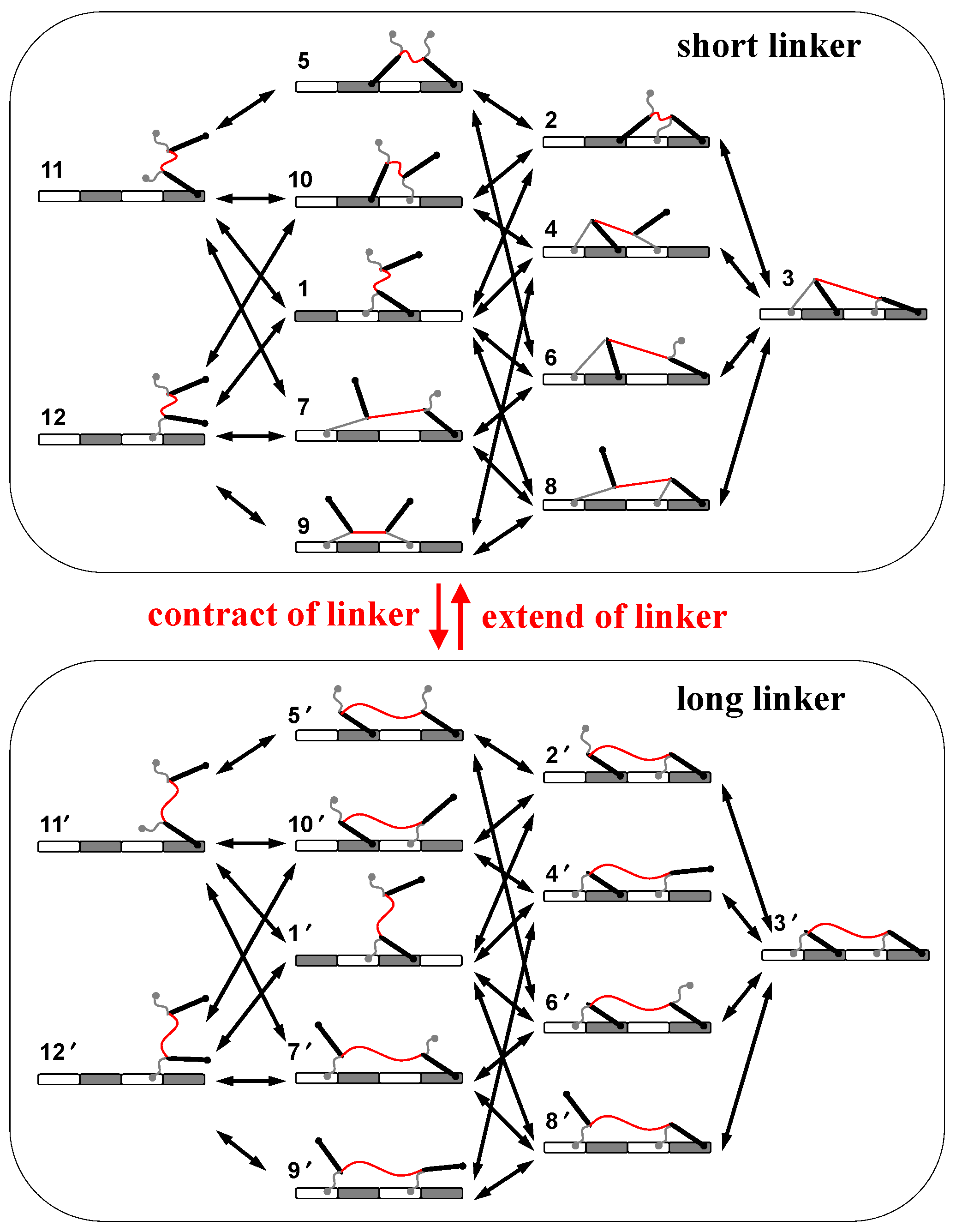
Based on the mechanics of the motor, a mechanical–kinetic model is developed for analyzing performances of the motor. All motor-track binding states are considered in the kinetics, including 12 states in total (Figure 2). The contraction–extension operation switches the linker between two lengths, which generates two sets of such states (2 × 12 states in Figure 2). The binding or dissociation of a foot chain or a foot bone causes a transition within each set of states, while the operation causes a transition between the two sets of states (Figure 2). The overall kinetic network contains (Figure 2) all possible pathways with the two opposite moving directions for the motor’s stepping-along track and thus is used to test the possibility of biased motion.

Figure 2.
Kinetic network of the motor. Shown are possible motor-track binding states for short linker (upper box) and long linker (lower box). The red arrows indicates operation-caused transitions between the two ensembles. The black arrows indicates transitions within either ensemble.
Transitions within each set of states are spontaneous processes that are assumed reversible and obey the detailed-balance condition. Namely kij/kji = eΔFij/kBT, where kij is the transition rate from state i to state j, and ΔFij is the free-energy difference between state i and state j. The condition ensures the equilibrium when no operation is applied. Within each set of states, the dissociation rates for foot-chain and foot-bone are assumed in the form of kd0·e fp·ld/kBT, where fp is the pulling force on the chain or bone; ld is the force-coupling distance, and kd0 is the zero-force rate. The rates for the reverse binding are derived from the detailed-balance condition via ΔFij. fp and ΔFij for all the motor-track states are calculated by the mechanical model. As for the operation, the contraction and extension of the linker is assumed to be enforced externally, and thereby a constant rate is assigned to all the inter-sets transitions that are caused by the operation.
Performance of the motor is evaluated at a steady state. Since all transition rates are clearly defined, the steady-state solution for the probabilities (pi for state i) of each motor-track state is derived via a master equation, namely dpi/dt = ∑j (pjkji − pikij) = 0. The average speed and directional fidelity of the motor are derived from the solution of the probability (pi) (which will be shown later).
3. Results
3.1. Selective Foot Detachment and Biased Binding
The designed asymmetry inside the motor-track system gives rise to the biased detachment and binding behavior of the motor. For a two-foot bound state (Figure 1A), the contraction of the linker causes uneven strains to the two feet. For the front foot (towards the plus end of the track), the foot bone is pressed down towards the track and so is stabilized, but the foot chain is pulled (fchain) up away from the track and so is destabilized. For the rear foot (towards minus end of the track), the foot bone is pulled (flink) up away from the track, while the foot chain is relaxed. As a consequence, the chain of the front foot and the bone of the rear foot are engaged in a tug of war. Mechanical equilibrium requires fchain⋅sinα = flink⋅sinβ (Figure 1A). If the size parameters are chosen to ensure α > β, and thereby flink > fchain, the rear-foot bone tends to be preferentially dissociated. After the dissociation, the tug of war is between the two foot chains (Figure 1A). Similarly, if the size parameters are chosen properly, the rear-foot chain tends to be preferentially dissociated even if both binding components are equally stable on the track. Hence, the combined consequence is the selective detachment of the whole rear foot.
After rear-foot detachment, the one-foot bound state (state 1 in Figure 1B) is not stable yet. The free-energy hierarchy (Figure 1B) suggests that the detached foot bone will bind forward to form the most stable state (state 2 in Figure 1B) under the short linker. In contrast, backward binding forms less-stable states (state 3 or 4) than state 1, which is not likely. If linker extension occurs after state 2 is reached, the detached foot chain will bind to track to form the most stable state (state 3’) under the long linker. Hence, the motor-track system also facilitates a biased binding for the detached foot. If the contraction–extension operations are applied on the linker, the motor can make sustained forward steps along a working cycle of 3′→3→4→1→2→2′→3′ (Figure 1C). Parameters that produce the results are realistic for nanomotor systems (Table 1).

Table 1.
Parameters. The value of lp is derived from refs. [25,26].
3.2. Mechanistic Integration of Selective Foot Detachment and Biased Binding
Integration of the selective foot detachment and biased binding for unidirectional stepping is tested by the mechanical–kinetic model (Figure 2). The model considers all stepping pathways and motor-track binding states. If the both mechanisms function, stepping of the motor can be unidirectional. The directional fidelity (D) of the motor is defined by the net probability of forward steps over all steps [22,23], which is formulated below for this model:
Jij denotes the transition flux from state i to state j (Jij = pikij). Only detachment for an entire foot (e.g., 4→1 or 6→1 in Figure 2) and binding of a completely detached foot (e.g., 1→2 or 1→8 in Figure 2) are counted in Equation (1), as these transitions are real steps along the track. The “+” and “−” signs denote the stepping direction (forward or backward) of the transition. Unidirectional stepping occurs when D approaches one.
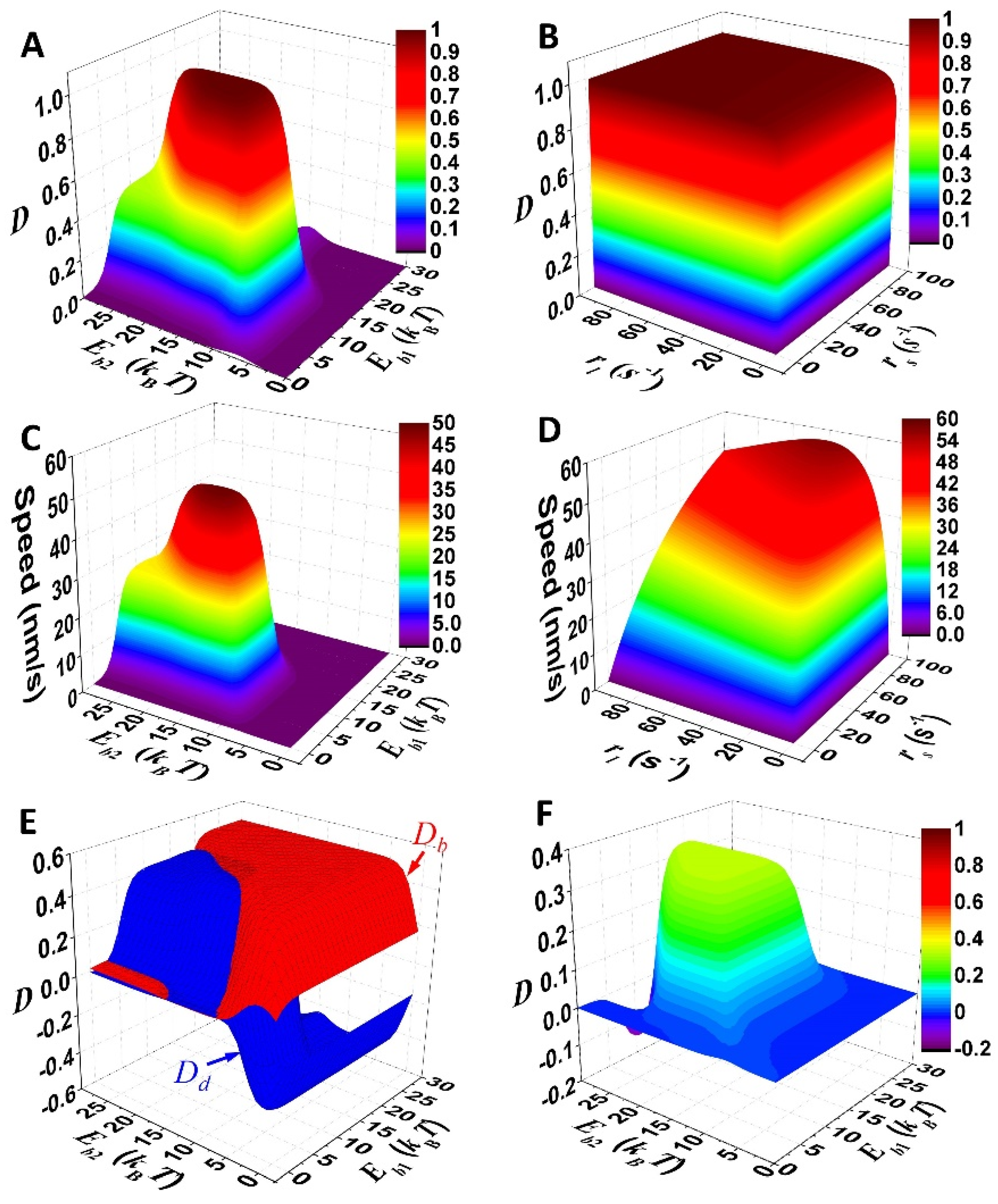
The binding energy of the foot as well as operation rates of the linker are scanned for testing whether unidirectional stepping is possible for the motor (Figure 3A,B). The result shows that the directional fidelity approaches one with binding energies (10–20 kBT) and operation rates (>10 s−1) that are applicable to nanomotors. For comparison, the speed of the motor is derived via v = ∑i pikijΔxij, where Δxij is the average displacement of the motor during the transition i→j. Dependences of the speed on the parameters (Figure 3C,D) qualitatively follow that of the directional fidelity (Figure 3A,B), which is rational as high speed occurs for unidirectional motility.

Figure 3.
Mechanistic integration of the motor. (A–D) Illustration of directional fidelity and speed of the motor. Operation rate of either linker contraction (rs) or extension (rl) is 50 s−1 for (A,C). Binding energy of either foot bone (Eb1) or chain (Eb2) is 12.5 kBT for (B,D). Other parameters are listed in Table 1. (E) Contributions of foot detachment (Dd) and binding (Db) to overall D is shown. (F) Shown is directional fidelity of the motor with zero force-coupling distance (ld = 0) for both foot bone and foot chain. Parameters used for (E) and (F) are the same as for (A) and (C), except ld = 0 for (F).
For direct testing of the integration, the total directional fidelity (D) is decomposed into the contributions from foot detachment (Dd) and binding (Db). The contributions are defined by Dd = (∑ij − ∑ij )/(∑ij + ∑ij ) and Db = (∑ij − ∑ij )/(∑ij + ∑ij ), where “d” and “b” denote transitions for foot detachment and binding, respectively. It is not difficult to derive D = Dd + Db. The decomposition shows that both Dd and Db are limited below 0.5 (Figure 3E), which suggests that D is capped below 0.5 if only one mechanism works. Moreover, the selective-foot detachment is deliberately discarded in modeling by assigning a zero force-coupling distance (ld = 0) to both the foot chain and foot bone. Solely by the biased-binding mechanism, the directional fidelity of the motor cannot exceed 0.5 (Figure 3F). Thus, the total D that approaches one (Figure 3A,B) is attributed to integration of the selective foot detachment and biased binding.
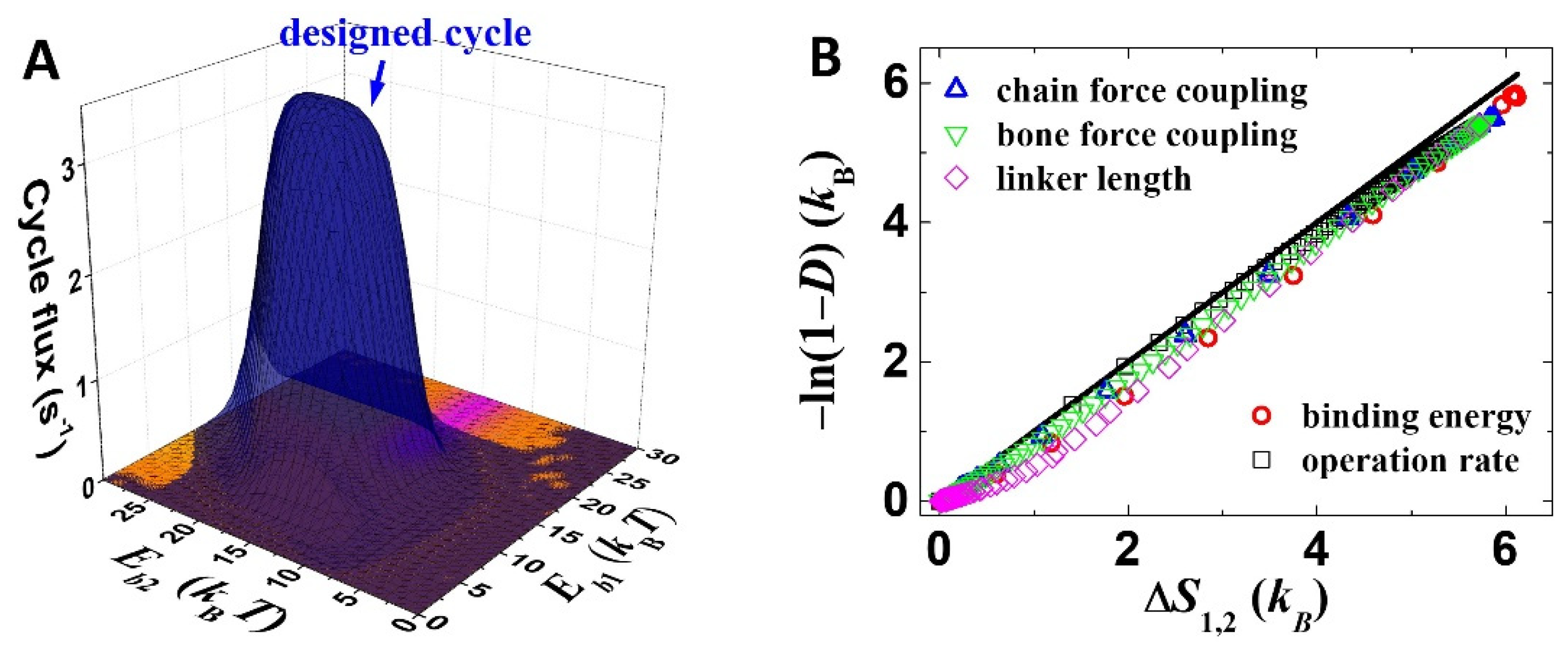
For identifying an exact stepping process out of the many possibilities in the 2 × 12 kinetic network (Figure 2), the overall kinetics is decomposed into contributions from individual cycles (by the method from ref. [27]). The designed cycle (Figure 1C) largely dominates the overall working of the motor (Figure 4A). One can find that the binding-energy dependence of the cycle flux of the designed cycle (Figure 4A) is consistent with that of the directional fidelity (Figure 3A) and the speed (Figure 3C), and the maximum cycle flux (~3.5 s−1 in Figure 4A) matches the maximum speed (~50 nm·s−1 in Figure 3C, 14 nm step size). These results confirm that the selective foot detachment and biased binding are integrated within the designed working cycle.

Figure 4.
Working process analysis. (A) Cycle fluxes of the designed cycle (blue) as well as competing cycles (other colors) are shown. The competing cycles include 3′→3→8→1→2→2′→3′,3′→ 3→6→1→2→2′→3′, 3′→3→2→1→1′→4′→3′ and 3′→3→4→1→8→8′→3′. Parameters are kept the same as Figure 3A. (B) The line indicates y = x, and the symbols are results from the mechanical–kinetic model. The modeling results are varied by adjusting binding energies (Eb1 and Eb2), operation rates (rl and rs), force-coupling distances of the foot chain and bone (ld) and linker length (lc).
3.3. Optimization of the Motor
The shown result suggests that the improvement of directional fidelity can bring the improvement of other performance, e.g., speed (Figure 3). From this section, the optimization of the motor is conducted by maximizing the directional fidelity, and thermodynamic correlation between the directional fidelity and other performances, e.g., work production and speed, is analyzed. Before the optimization, thermodynamics of directional fidelity are analyzed first. The study from ref. [23] proposes that the directional fidelity of a bipedal motor depends on entropy productions accompanying rear foot detachment and forward binding. The relation is expressed below for the motor of this study:
Here, ΔSij = kBln(pikij/pjkji) [28,29], which is the average entropy production of a transition from state i to state j. Equation (2) uses transitions 4→1 and 1→2 to represent all the rear foot detachment processes and forward binding processes. This approximation is apply because the designed cycle dominates the working of the motor (Figure 4A). For most chosen parameters in this study, ΔS4,1 is larger than ΔS1,2. Thus, Equation (2) is well approximated into D ≈ 1 − e−ΔS1,2/kB or, inversely, ΔS1,2 ≈ −kBln(1 − D). The equality is tested by computation results from the mechanical–kinetic model (Figure 4B), which achieves remarkable consistency. The computation result is derived by scanning the binding energies, force-coupling lengths, linker length and operation rates over sufficient ranges (Figure 4B). Small deviations from the D-ΔS1,2 equality appear, which is reasonable since the equality is exact for strictly a single cycle plus an infinitely large ΔS4,1, and both conditions are not perfectly met by the model. The analysis suggests that the quantity of entropy productions can be potentially key for the thermodynamic analysis of the optimization.
For the optimization of the motor, the directional fidelity is maximized via scanning parameters of the system, including binding energies (Eb1 and Eb2), dissociation rates (kd0), force-coupling distances (ld) and operation rates (rl and rs) (Table 2). The work production of the motor after the optimization is analyzed. For output work, a load force is attached to the motor in modeling. The load force is attached in the middle of the linker, as is often the case for force-clamp experiments of biological motors. The load force modifies the inner strain of the motor (fp) as well as the free energy gaps between the 24 motor-track states (ΔFij). The quantities are still obtained by the mechanical model, which in turn govern the kinetics as for the zero-load case. Beside the inner free energy of the motor, the load force build an external potential field for the motor, which contributes an extra amount of free energy, namely f·Δxij, where f is the load, and Δxij is the displacement of the motor in transition i→j. The extra free energy is also considered in modeling.
Table 2.
Parameters after optimization at zero load. The parameters that maximized directional fidelity at zero load are shown in the table. Scanning ranges of the parameters for the maximization are 0 to 30 kBT for binding energies, 0.1 to 1 s−1 for dissociation rates (kd0), 0.1 to 1 nm for force-coupling distance (ld) and 1 to 107 s−1 for operation rates.
As for the first step, the scanning of parameters for the maximization of directional fidelity is performed when no load is attached. Performances of the motor before and after the zero-load optimization are compared (Figure 5). Before the optimization, the directional fidelity of the motor under a zero load was already close to one, and thus the improvement of the directional fidelity after the optimization is rather limited (Figure 5A). However, the directional fidelity of the motor extends, obviously, further against the load after the optimization (Figure 5A). Hence, the motor achieves a larger stall force (the force stops the motor (D = 0)) and maximum output work (stall force multiplied by the step size) after the optimization. The result indicates that the work production of the motor is largely improved after the zero-load optimization.

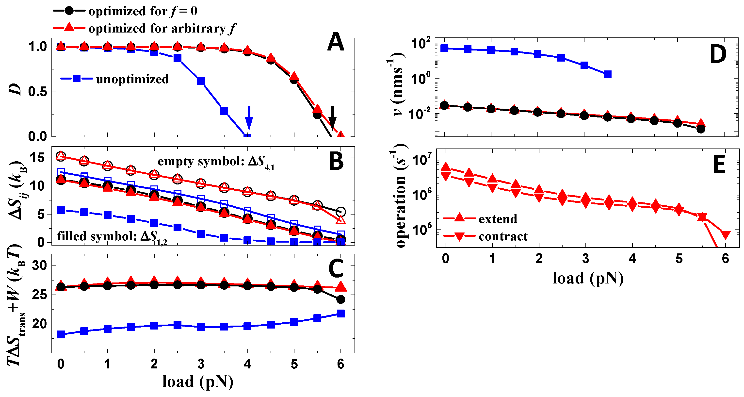
Figure 5.
Optimality of the motor. (A) Load dependences of the directional fidelity for cases before and after the optimization. Parameters of the cases are listed in Table 1 and Table 2, except that before the optimization, the binding energies are 15 kBT for both foot bone and chain. The arrows mark the stall forces. (B) Load dependences of ΔS4,1 and ΔS1,2 for cases shown in (A). (C) Load dependences of summation of TΔS4,1, TΔS1,2 (ΔStrans = ΔS4,1 + ΔS1,2) and output work (W = fd0 with f as the load force and d0 as the motor step size) for the cases shown in (A). (D) Load dependences of the speed for the cases shown in (A). (E) Load dependences of contraction and extension rates (rl and rs) for the case optimized for arbitrary load.
The correlation between work production and zero-load directional fidelity is analyzed. After the zero-load optimization, ΔS4,1 and ΔS1,2 at zero load are increased significantly (Figure 5B). Note that the directional fidelity only relies on the two entropy productions (Equation (2)). However, after the optimization, ΔS4,1 and ΔS1,2 remain linearly reduced against the load with an approximately conserved slope (Figure 5B). The conserved load dependences naturally lead to larger stall forces if the values of ΔS4,1 and ΔS1,2 at zero load are increased. One can find that the stall force is close to the location where ΔS1,2 approaches zero (Figure 5B). This is because either a zero ΔS4,1 or zero ΔS1,2 leads to zero directional fidelity (Equation (2), and ΔS1,2 is just the smaller one out of the two entropy productions. For understanding the improvement of work production from a physics perspective, the total amount of TΔS4,1 (energy dissipation of rear foot detachment), TΔS1,2 (energy dissipation of forward binding) and output work (W = fd0) are derived (Figure 5C). As the result, the total amount of energy remains stable against load (Figure 5C). Since TΔS4,1 and TΔS1,2 reduces linearly against load, and the output work increases linearly with load, the stable total amount of energy suggests it is the energy used for driving rear-foot detachment (TΔS4,1), and forward binding (TΔS1,2) converts to work after the load is attached. The stable total amount of energy also suggests that other processes (transitions) in the working cycle are not likely relevant to work production. Hence, directional fidelity and work production of the motor are correlated via the two entropy productions that contribute to both of the performances. The result indicates the directional fidelity is a meaningful quantity for the optimization of the motor.
Secondly, after the zero-load optimization, a load-dependent optimization is further conducted to the motor, in which the directional fidelity of the motor under a finite load is further optimized by scanning the two operation rates. The scanning generates two load-dependent operation rates (Figure 5E), which further maximizes the directional fidelity. Such load-dependent driving is possible for biological nanomotors [30] because load can influence the catalysis of the fuel molecule that drives the motor. However, the improvements brought by the load-dependent optimization in directional fidelity (Figure 5A), stall force (Figure 5A), TΔS4,1, TΔS1,2 (Figure 5B,C) and speed (Figure 5D) are marginal. Note that the resultant load dependences of the operation rates (Figure 5E) after the optimization are continuous and smooth, which produces locally maximized directional fidelity. Hence, the zero-load optimization approximately achieves the load-dependent optimization. The effect is understandable if considering that only TΔS4,1 and TΔS1,2 contribute to directional fidelity and work production, and their load dependences remain stable against the adjustment of operation rates for all cases (before optimization, zero-load optimization and load-dependent optimization) (Figure 5B).
3.4. Speed-Directional Fidelity Tradeoff
After optimization, despite the improvement of directional fidelity and stall force, the speed of the motor, however, drops more than two magnitudes (Figure 5D). For the analysis of the speed drop, a trace of optimization is recorded (Figure 6A). The trace is produced by scanning the binding energies (Eb1 and Eb2) and operation rates (rl and rs) with a performance point recorded only if the present directional fidelity is higher than the preceding one. The parameters of zero-load dissociation rates (kd0) and force-coupling distances (ld) are not applied in the optimization because these parameters can directly amplify or reduce all transition rates for stepping (detachment and binding), which strongly destabilizes the value of speed. When the directional fidelity of the motor increases along the present trace (Figure 6A), the speed also increases. However, the increasing trend remains up to D~0.99. When the fidelity further approaches one, the speed decreases steeply toward zero (Figure 6A).
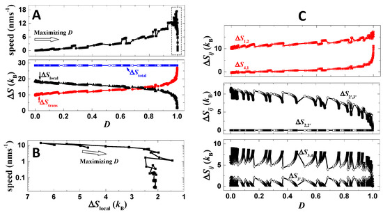
Figure 6.
Speed-directional fidelity tradeoff. (A) Shown are the directional fidelity, speed and entropy productions of the motor following a trace of optimization (no load is applied). During the optimization, the binding energies and operation rates are scanned linearly. The trace starts from a poor case of zero directional fidelity by parameters listed in Table 1, except that zero operation rates are used. The empty arrow shows the evolution direction of the trace. ΔStrans is the total amount of fidelity-relevant entropy productions, namely ΔStrans = ΔS1,2 + ΔS4,1, and ΔSlocal is the total amount of fidelity-irrelevant entropy productions, namely ΔSlocal = ΔS2,2’ + ΔS2’,3’ + ΔS3’,3 + ΔS3,4. ΔStotal is the sum of ΔStrans and ΔSlocal. (B) The panel shows the last part of the trace (marked by dash-line box in (A)) where the speed decreases from 18 nms−1 to 0. The trace is shown with ΔSlocal as x axis. (C) Shown are still the optimization trace, but displayed with entropy productions as y axis.
During the maximization of directional fidelity, the speed of the motor is not controlled by any procedure, and thus both increase and decrease of the speed can be seen in the details of the trace. In fact, the detailed functional form of the D-v trace (Figure 6A) depends on the choice of how the parameters are scanned for the optimization. However, the shown increasing trend of speed vs. directional fidelity for small directional fidelity is understandable, namely higher directional fidelity requires higher probability for forward steps and lower probability for backward steps, which benefits the speed. The trend is consistent with the result shown in Figure 3A–D. The speed drop when the directional fidelity approaches one is also understandable, which is explained by the thermodynamic analysis shown below.
The dependence of directional fidelity on entropy productions is approximated by Equation (2), and the dependence for speed is approximated by the equation below,
Here the summation of ij only include the six transitions along the designed cycle (Figure 1C), as taking dominance of the cycle for approximation. The derivation of Equation (3) can be found in ref. [31]. Unlike the directional fidelity (Equation (2)), which only relies on entropy productions of rear-foot detachment (ΔS4,1) and forward binding (ΔS1,2), the speed depends on all the six entropy productions of the cycle (Equation (3)) and decays to zero if any one of the six entropy productions approaches zero. Thus, finite speed requires a certain balance among all six entropy productions if the total amount is limited, and a crisis for speed breaks out if all energy is exhausted solely by ΔS4,1 and ΔS1,2 for raising the directional fidelity toward the ultimate limit.
Results from the mechanical–kinetic model support the above analysis. Along the entire trace, the total entropy production of the six transitions (ΔStotal) remains a constant (Figure 6A). This is because the operation is unchanged during the optimization and thus provides constant total driving energy to the system. When the directional fidelity increases along the trace, the fidelity-relevant entropy production (ΔStrans = ΔS4,1 + ΔS1,2) increases as expected, while the fidelity-irrelevant entropy production (ΔSlocal = ΔS2,2’ + ΔS2’,3’ + ΔS3’,3 + ΔS3,4) decreases as the total entropy production (ΔStotal) is limited (Figure 6A). When D approaches extremely close to one, ΔStrans indeed exhausts almost all energy, which produces a crisis for ΔSlocal and in turn for speed (Figure 6A). The speed–ΔSlocal plot (Figure 6B) clearly displays that the speed drops more than two magnitudes when ΔSlocal decreases from 3 kB to 2 kB, while the speed decreases with drastically reduced pace when ΔSlocal decreases from 7 kB to 3 kB. Detailed variations of each entropy production are summarized in Figure 6C. The above speed-directional fidelity tradeoff is consistent with the reported study [23] based on single-cycle kinetics, while here the tradeoff is displayed based on a mechanical model with all possible stepping pathways considered and detailed processes showing how the tradeoff occurs.
4. Discussion
4.1. Implementation of the Motor-Track System
The design of the motor-track system is implementable in experiments. One probable option for implementation is assembling from predesigned DNA sequences. Tracking with compound binding sites has been demonstrated in experiments [10,11,12]. The contraction–extension operation can be implemented by alternately forming and breaking a folded structure of DNA [32,33,34,35,36,37] or by directly varying the contour length if the DNA strands are embedded with light-responsive moieties [38,39]. Examples of the operation can be found in reported experimental systems [11]. The unique design in the present system is the compound foot plus the rigid component of the foot bone, which have not been used as a single foot in experiments. The compound foot can be implemented by designing forking at either end of a double-strand DNA, while one overhang strand from the forking must be duplexed with the complementary strand, as a DNA duplex is rigid enough for being the foot bone. The structure of forking was used as two feet in early types of DNA nanomotors [40].
Options [11,41,42] for testing the proposed selective-foot detachment and biased binding are also reachable. One option [11] is attaching different dye molecules to different binding sites of the track and quencher molecules to both feet of the motor. Due to that the dye molecules can emit fluorescence, and the quencher can block the fluorescence, the rear/front foot detachment as well as forward/backward binding can be, respectively, marked by different variations of the fluorescence. A reliable simulation method [43] also can be found for the testing. Examples of such testing on other DNA nanomotor systems have been reported [41,42].
The well-known Brownian motor model [44] may provide a simple test of the speed- directional fidelity tradeoff. In the model, a directional flow of particle can be generated by flashing a ratchet potential. If an optimization trace (similar to Figure 6A) of the Brownian motor is generated by scanning the flashing rate from slow to fast, one can find that the trace will start from zero speed and zero directional fidelity because the system maintains equilibrium under super slow driving. Both speed and directional fidelity will increase with the flashing rate as the model can generate a directional flow at a finite flashing rate. However, when the flashing rate becomes superfast, the speed will decrease, as the particle can only go across the front barrier when the ratchet is shut down, and the crossing time under superfast flashing is too short for successive crossing. Meanwhile, the directional fidelity is not likely to reduce, as the ratchet potential is asymmetric in space and backward flow is always much weaker than the forward one under fast flashing rate.
4.2. Motor Optimality
Experimental data of bionanomotor kinesin [23] and F1-ATPase [24] show that the directional fidelity of a motor can be maximized throughout a pre-stalemate load. Since great research effort is spent on producing artificial nanomotors in the laboratory, a universal optimized artificial nanomotor is desirable for widespread applications in nanotechnology. However, to realize universal optimality in artificial system seems difficult because a motor is required to be optimized for arbitrary loads. An interesting result from this study is that the universal optimality is approximately approached by the zero-load optimization. The result suggests that adjusting a motor’s construction and operation associated with zero-load performance is likely the key for the optimization of a motor.
The kinetic model (Figure 2) in this study considers all the working pathways consisting of the 2 × 24 motor-track state rather than singly the designed cycle. The multiple pathways can bring energy dissipation to the motor, as driving energy might be wasted by futile cycles or backward-moving cycles. Please note that energy dissipation caused by the forward displacement of a motor (e.g., TΔS4,1 and TΔS1,2) should not be simply counted as pure dissipation or waste, because the energy can be converted to work after load is attached. If a single cycle is used in modeling, the maximum work production of a motor usually matches the input driving to the cycle, and thus no real waste of energy is caused. The single-cycle modeling is often applied on biological nanomotors, which is reasonable as it is a good approximation for highly efficient nanomotors. However, the multi-pathway modeling of this study suggests that only the energy used for generating actual displacement (rear-foot detachment and forwarding binding) can be converted to work after the load is attached, while energy used for other processes is likely dissipated. The result is consistent with classic thermodynamics for heat engines where only the energy used for cylinder expansion can convert to work, while the energy used for other processes, such as changing temperature, is irrelevant to work production. The information might be useful to studies on nanomotors as it specifies the processes for work production, which is unlikely to be given by single-cycle modeling.
5. Summary
In summary, a simple bipedal motor was designed from a polymer structure that forks at either end into a soft and a rigid binding component. The linear track only requires alternate binding sites for the soft and the rigid binding components. When the size of the motor-track system is properly chosen, the binding mechanics coupled with the alternating extension and contraction of the inter-feet linker give rise to the directional motion of the motor. Firstly, the mechanisms rectify the motor’s motion to directionally include selective foot detachment and biased binding. Neither of the two mechanisms is assumed by hand. Each of the two mechanisms alone rectifies directional motion, but the motor performance based on a single mechanism is capped by a general limit (0.5) in terms of directional fidelity. The simplistic motor-track system is able to additively integrate the mechanisms by coupling them sequentially into the energy-consuming cycle, which promotes the motor’s performance beyond the limit. Secondly, a motor can be optimized by maximizing the directional fidelity, which promotes the working production. A motor’s directional fidelity can be optimized simultaneously for different values of external loads by adjusting parameters associated with the motor’s physical construction regardless of external operation. Thirdly, when a motor’s directional fidelity becomes perfect, its speed approaches infinitely slowness. Such a speed-directional fidelity tradeoff is caused by an energetic crisis: optimal directional fidelity maximizes entropy productions of some transitions but abolishes other speed-limiting transitions for a finite amount of energy supply. When the speed-limiting entropy productions gain finite values linearly, the motor’s speed recovers exponentially from zero.
Funding
This research was funded by National Natural Science Foundation of China under grant No. 11904278, by the Science and Technology Department of Shaanxi Province under grant Nos. 2020JQ-612 and 2019JQ-317, by the Education Department of Shaanxi Province under grant No. 19JK0574 and by the Project of The Youth Innovation Team of Shaanxi Universities.
Institutional Review Board Statement
Not applicable.
Informed Consent Statement
Not applicable.
Data Availability Statement
Not applicable.
Conflicts of Interest
The author declare no conflict of interest.
References
- Simmel, F.C.; Yurke, B.; Singh, H.R. Principles and Applications of Nucleic Acid Strand Displacement Reactions. Chem. Rev. 2019, 119, 6326–6369. [Google Scholar] [CrossRef] [PubMed]
- Feringa, B.L. The Art of Building Small: From Molecular Switches to Motors (Nobel Lecture). Angew. Chem.-Int. Ed. 2017, 56, 11059–11078. [Google Scholar] [CrossRef] [PubMed] [Green Version]
- Kassem, S.; van Leeuwen, T.; Lubbe, A.S.; Wilson, M.R.; Feringa, B.L.; Leigh, D.A. Artificial molecular motors. Chem. Soc. Rev. 2017, 46, 2592–2621. [Google Scholar] [CrossRef] [PubMed] [Green Version]
- Wilson, M.R.; Sola, J.; Carlone, A.; Goldup, S.M.; Lebrasseur, N.; Leigh, D.A. An autonomous chemically fuelled small-molecule motor. Nature 2016, 534, 235. [Google Scholar] [CrossRef] [Green Version]
- Erbas-Cakmak, S.; Fielden, S.D.P.; Karaca, U.; Leigh, D.A.; McTernan, C.T.; Tetlow, D.J.; Wilson, M.R. Rotary and linear molecular motors driven by pulses of a chemical fuel. Science 2017, 358, 340–343. [Google Scholar] [CrossRef] [Green Version]
- Omabegho, T.; Sha, R.; Seeman, N.C. A bipedal DNA Brownian motor with coordinated legs. Science 2009, 324, 67–71. [Google Scholar] [CrossRef] [Green Version]
- Green, S.J.; Bath, J.; Turberfield, A.J. Coordinated chemomechanical cycles: A mechanism for autonomous molecular motion. Phys. Rev. Lett. 2008, 101, 238101. [Google Scholar] [CrossRef] [Green Version]
- Yin, P.; Choi, H.M.T.; Calvert, C.R.; Pierce, N.A. Programming biomolecular self-assembly pathways. Nature 2008, 451, 318–322. [Google Scholar] [CrossRef] [Green Version]
- Tian, Y.; He, Y.; Chen, Y.; Yin, P.; Mao, C. A DNAzyme that walks processiviely and autonomously along a one-dimensional track. Angew. Chem. Int. Ed. 2005, 44, 4355–4358. [Google Scholar] [CrossRef]
- Cheng, J.; Sreelatha, S.; Hou, R.Z.; Efremov, A.; Liu, R.C.; van der Maarel, J.R.C.; Wang, Z.S. Bipedal Nanowalker by Pure Physical Mechanisms. Phys. Rev. Lett. 2012, 109, 238104. [Google Scholar] [CrossRef] [Green Version]
- Loh, I.Y.; Cheng, J.; Tee, S.R.; Efremov, A.; Wang, Z. From Bistate Molecular Switches to Self-Directed Track-Walking Nanomotors. Acs Nano 2014, 8, 10293–10304. [Google Scholar] [CrossRef] [PubMed]
- Liu, M.H.; Cheng, J.; Tee, S.R.; Sreelatha, S.; Loh, I.Y.; Wang, Z.S. Biomimetic Autonomous Enzymatic Nanowalker of High Fuel Efficiency. Acs Nano 2016, 10, 5882–5890. [Google Scholar] [CrossRef] [PubMed]
- Hu, X.; Zhao, X.; Loh, I.Y.; Yan, J.; Wang, Z. Single-molecule mechanical study of an autonomous artificial translational molecular motor beyond bridge-burning design. Nanoscale 2021, 13, 13195–13207. [Google Scholar] [CrossRef] [PubMed]
- Gu, H.; Chao, J.; Xiao, S.J.; Seeman, N.C. A proximity-based programmable DNA nanoscale assembly line. Nature 2010, 465, 202–206. [Google Scholar] [CrossRef]
- Thubagere, A.J.; Li, W.; Johnson, R.F.; Chen, Z.; Doroudi, S.; Lee, Y.L.; Izatt, G.; Wittman, S.; Srinivas, N.; Woods, D.; et al. A cargo-sorting DNA robot. Science 2017, 357, eaan6558. [Google Scholar] [CrossRef] [Green Version]
- Lund, K.; Manzo, A.J.; Dabby, N.; Michelotti, N.; Johnson-Buck, A.; Nangreave, J.; Taylor, S.; Pei, P.; Stojanovic, M.N.; Walter, N.G.; et al. Molecular robots guided by prescriptive landscapes. Nature 2010, 465, 206–210. [Google Scholar] [CrossRef] [Green Version]
- Wickham, S.F.J.; Bath, J.; Katsuda, Y.; Endo, M.; Hidaka, K.; Sugiyama, H.; Turberfield, A.J. A DNA-based molecular motor that can navigate a network of tracks. Nat. Nanotechnol. 2012, 7, 169–173. [Google Scholar] [CrossRef]
- He, Y.; Liu, D.R. Autonomous multistep organic synthesis in a single isothermal solution mediated by a DNA walker. Nat. Nanotechnol. 2010, 5, 778–782. [Google Scholar] [CrossRef] [Green Version]
- Meng, W.; Muscat, R.A.; McKee, M.L.; Milnes, P.J.; El-Sagheer, A.H.; Bath, J.; Davis, B.G.; Brown, T.; O’Reilly, R.K.; Turberfield, A.J. An autonomous molecular assembler for programmable chemical synthesis. Nat. Chem. 2016, 8, 542–548. [Google Scholar] [CrossRef]
- De Bo, G.; Gall, M.A.Y.; Kuschel, S.; De Winter, J.; Gerbaux, P.; Leigh, D.A. An artificial molecular machine that builds an asymmetric catalyst. Nat. Nanotechnol. 2018, 13, 381. [Google Scholar] [CrossRef]
- Clancy, B.E.; Behnke-Parks, W.M.; Andreasson, J.O.L.; Rosenfeld, S.S.; Block, S.M. A universal pathway for kinesin stepping. Nat. Struct. Mol. Biol. 2011, 18, 1020–1027. [Google Scholar] [CrossRef] [PubMed] [Green Version]
- Efremov, A.; Wang, Z.S. Maximum directionality and systematic classification of molecular motors. Phys. Chem. Chem. Phys. 2011, 13, 5159–5170. [Google Scholar] [CrossRef] [PubMed]
- Efremov, A.; Wang, Z. Universal optimal working cycles of molecular motors. Phys. Chem. Chem. Phys. 2011, 13, 6223–6233. [Google Scholar] [CrossRef] [PubMed]
- Hou, R.; Wang, Z. Role of directional fidelity in multiple aspects of extreme performance of the F-1-ATPase motor. Phys. Rev. E 2013, 88, 022703. [Google Scholar] [CrossRef] [Green Version]
- Wang, Z.S.; Makarov, D.E. Rate of intramolecular contact formation in peptides: The loop length dependence. J. Chem. Phys 2002, 117, 4591–4593. [Google Scholar] [CrossRef]
- Wang, Z.S.; Plaxco, K.W.; Makarov, D.E. Influence of local and residual structures on the scaling behavior and dimensions of unfolded proteins. Biopolymers 2007, 86, 321–328. [Google Scholar] [CrossRef]
- Hill, T.L. Free Energy Transduction and Biochemical Cycle Kinetics; Springer: New York, NY, USA, 1989. [Google Scholar]
- Seifert, U. Entropy Production along a Stochastic Trajectory and an Integral Fluctuation Theorem. Phys. Rev. Lett. 2005, 95, 040602. [Google Scholar] [CrossRef] [Green Version]
- Schnakenberg, J. Network theory of microscopic and macroscopic behavior of master equation systems. Rev. Mod. Phys 1976, 48, 571–585. [Google Scholar] [CrossRef]
- Visscher, K.; Schnitzer, M.J.; Block, S.M. Single kinesin molecules studied with a molecular force clamp. Nature 1999, 400, 184–189. [Google Scholar] [CrossRef]
- Hou, R.; Loh, I.Y.; Li, H.; Wang, Z. Mechanical-Kinetic Modeling of a Molecular Walker from a Modular Design Principle. Phys. Rev. Appl. 2017, 7, 024020. [Google Scholar] [CrossRef]
- Alberti, P.; Mergny, J.L. DNA duplex-quadruplex exchange as the basis for a nanomolecular machine. Proc. Natl. Acad. Sci. USA 2003, 100, 1569–1573. [Google Scholar] [CrossRef] [PubMed] [Green Version]
- Lubrich, D.; Lin, J.; Yan, J. A contractile DNA machine. Angew. Chem. Int. Ed. 2008, 47, 7026–7028. [Google Scholar] [CrossRef] [PubMed]
- Hamad-Schifferli, K.; Schwartz, J.J.; Santos, A.T.; Zhang, S.; Jacobson, J.M. Remote electronic control of DNA hybridization through inductive coupling to an attached metal nanocrystal antenna. Nature 2002, 415, 152–155. [Google Scholar] [CrossRef] [PubMed]
- Liedl, T.; Simmel, F.C. Switching the conformation of a DNA molecule with a chemical oscillator. Nano Lett. 2005, 5, 1894–1898. [Google Scholar] [CrossRef]
- Xiao, X.; Plakos, K.J.I.; Lou, X.; White, R.J.; Qian, J.; Plaxco, K.W.; Soh, H.T. Fluorescence detection of single-nucleotide polymorphisms with a single self-complementary, triple-stem DNA probe. Angew. Chem. Int. Ed. 2009, 48, 4354–4358. [Google Scholar] [CrossRef] [Green Version]
- Vallee-Belisle, A.; Ricci, F.; Plaxco, K.W. Thermodynamic basis for the optimization of binding-induced biomolecular switches and structure-switching biosensors. Proc. Natl. Acad. Sci. USA 2009, 106, 13802–13807. [Google Scholar] [CrossRef] [Green Version]
- Hugel, T.; Holland, N.B.; Cattani, A.; Moroder, L.; Seitz, M.; Gaub, H.E. Single-molecule optomechanical cycle. Science 2002, 296, 1103–1106. [Google Scholar] [CrossRef]
- Liang, X.; Mochizuki, T.; Asanuma, H. A supra-photoswitch involving sandwiched DNA base pairs and azobenzenes for light-driven nanostructures and nanodevices. Small 2009, 5, 1761–1768. [Google Scholar] [CrossRef]
- Sherman, W.B.; Seeman, N.C. A precisely controlled DNA biped walking device. Nano Lett. 2004, 4, 1203–1207. [Google Scholar] [CrossRef]
- Tee, S.R.; Hu, X.; Loh, I.Y.; Wang, Z. Mechanosensing Potentials Gate Fuel Consumption in a Bipedal DNA Nanowalker. Phys. Rev. Appl. 2018, 9, 034025. [Google Scholar] [CrossRef]
- Ouldridge, T.E.; Hoare, R.L.; Louis, A.A.; Doye, J.P.K.; Bath, J.; Turberfield, A.J. Optimizing DNA Nanotechnology through Coarse-Grained Modeling: A Two-Footed DNA Walker. ACS Nano 2013, 7, 2479–2490. [Google Scholar] [CrossRef] [PubMed] [Green Version]
- Ouldridge, T.E.; Louis, A.A.; Doye, J.P.K. Structural, mechanical, and thermodynamic properties of a coarse-grained DNA model. J. Chem. Phys. 2011, 134, 085101. [Google Scholar] [CrossRef] [PubMed] [Green Version]
- Astumian, R.D. Thermodynamics and kinetics of a Brownian motor. Science 1997, 276, 917–922. [Google Scholar] [CrossRef] [PubMed] [Green Version]

Publisher’s Note: MDPI stays neutral with regard to jurisdictional claims in published maps and institutional affiliations. |
© 2022 by the author. Licensee MDPI, Basel, Switzerland. This article is an open access article distributed under the terms and conditions of the Creative Commons Attribution (CC BY) license (https://creativecommons.org/licenses/by/4.0/).