The Franson Experiment as an Example of Spontaneous Breaking of Time-Translation Symmetry

Abstract

We describe an explicit statistical model of local hidden variables that reproduces the predictions of quantum mechanics for the ideal Franson experiment and sheds light on the physical mechanisms that might be involved in the actual experiment. The crux of our model is the spontaneous breaking of time-translation gauge symmetry by the hidden configurations of the pairs of photons locked in time and energy involved in the experiment, which acquire a non-zero geometric phase through certain cyclic transformations.

1. Introduction

It is widely accepted wisdom that quantum phenomena cannot be fully described within the framework of any physical theory that shares the same notions of reality and relativistic causality that we acknowledge as a given in our classical descriptions of the macroscopic world [1]. This wisdom is precisely formulated through the Bell theorem on the attainable correlations between the outcomes of polarization measurements performed on pairs of photons prepared in a singlet polarization state [2,3]. The theorem draws a solid line (the Bell inequality) that allows experimentally discriminating between the predictions of quantum mechanics for these correlations and those of models of local hidden variables that fulfill certain physically intuitive requirements [4,5,6,7].

In a series of recent papers, we have shown, however, that the proof of the Bell theorem relies crucially on a subtle implicit assumption that is not required by fundamental physical principles and, therefore, the Bell inequality does not necessarily hold for models of local hidden variables that do not comply with the said unjustified assumption [8,9,10]. As a consequence, such models cannot be ruled out by the experimental evidence for the violation of the inequality [11,12,13].

The Franson experiment is often regarded as an alternative demonstration of the impossibility of describing quantum phenomena within the framework of any local model of hidden variables [14,15,16,17]. As in the case of the Bell experiment, it has been shown that certain features of the predictions of quantum mechanics for the Franson experiment cannot be reproduced within the framework of any model of local hidden variables that shares certain intuitive requirements [18,19,20,21].

In this paper we argue, however, that as in the case of the Bell experiment the models of local hidden variables whose predictions for the Franson experiment can be distinguished from those of quantum mechanics all share an assumption that is not required by any fundamental principle. Indeed, we explicitly describe a model of local hidden variables that does not comply with the disputed assumption; hence, it successfully reproduces the predictions of quantum mechanics for the experiment. The crux of our model is the spontaneous breaking of time-translation gauge symmetry by the hidden configurations of the pairs of photons locked in time and energy involved in the experiment, which acquire due to a holonomy a non-zero geometric phase through certain cyclic coordinate transformations. Let us stress that the gauge symmetry is spontaneously broken when each one of the possible hidden configurations of the pair of photons is considered separately (that is, for every single realization of the experiment), but it is statistically restored over the entire population of all possible hidden configurations (that is, over a long sequence of repetitions). Thus, the expected average correlations do only depend on the gauge-independent physical parameters that describe the settings of the experiment, in agreement with Elitzur’s theorem [22]. The model discussed here for the Franson experiment closely resembles the model of hidden variables introduced in [8,9,10] for the Bell experiment.

The paper is organized as follows. In section II, we present a (somewhat simplistic) description of the ideal Franson experiment within the framework of quantum mechanics and summarize its predictions (see [16] for a general review of optical tests of the Bell inequality). In section III, we present a detailed description of the setup of an actual experiment. In section IV, we describe a explicit model of local hidden variables that reproduces the predictions and the collected experimental data described in the two previous sections. Finally, in section V, we discuss and summarize our findings.

2. The Franson Experiment

In a Franson experiment, a source produces pairs of photons, A and B, for which their state is described by a wavefunction of the following form:

$$|\mathsf{\Psi }\rangle =\frac{|{\xi }_1{\rangle }^{\left(A\right)}+e^{i{\varphi }_A}{|{\xi }_2\rangle }^{\left(A\right)}}{\sqrt{2}}\otimes \frac{|{\xi }_1{\rangle }^{\left(B\right)}+e^{i{\varphi }_B}{|{\xi }_2\rangle }^{\left(B\right)}}{\sqrt{2}},$$

(1)

where $\left\{\right|{\xi }_1\rangle ,|{\xi }_2{\rangle \}}^{(A,B)}$ are orthonormal bases in their respective single-particle Hilbert spaces:

$${}^{\left(A\right)}{\langle {\xi }_1|{\xi }_2\rangle }^{\left(A\right)}={}^{\left(B\right)}{\langle {\xi }_1|{\xi }_2\rangle }^{\left(B\right)}=0,$$

(2)

and ${\varphi }_A$ and ${\varphi }_B$ are phases that, in principle, can be controlled and set at will.

A projective measurement is then performed on the pair of photons along the orthonormal basis in their joint Hilbert space $\left\{|c_1\rangle ,|c_2\rangle ,|c_3\rangle ,|c_4\rangle \right\}$ defined by the following vectors:

$$\begin{array}{ccc}\hfill |c_1\rangle ,& =& \frac{1}{\sqrt{2}}\left(|{\xi }_1{\rangle }^{\left(A\right)}\otimes |{\xi }_1{\rangle }^{\left(B\right)}+i|{\xi }_2{\rangle }^{\left(A\right)}\otimes {|{\xi }_2\rangle }^{\left(B\right)}\right),\hfill \\ \hfill |c_2\rangle ,& =& \frac{1}{\sqrt{2}}\left(|{\xi }_1{\rangle }^{\left(A\right)}\otimes |{\xi }_1{\rangle }^{\left(B\right)}-i|{\xi }_2{\rangle }^{\left(A\right)}\otimes {|{\xi }_2\rangle }^{\left(B\right)}\right),\hfill \\ \hfill |c_3\rangle ,& =& |{\xi }_1{\rangle }^{\left(A\right)}\otimes {|{\xi }_2\rangle }^{\left(B\right)},\hfill \\ \hfill |c_4\rangle ,& =& |{\xi }_2{\rangle }^{\left(A\right)}\otimes {|{\xi }_1\rangle }^{\left(B\right)},\hfill \end{array}$$

(3)

so that the probabilities $p_i=\langle \mathsf{\Psi }|c_i\rangle \langle c_i|\mathsf{\Psi }\rangle$ for each one of the four possible outcomes are given, respectively, by the following.

$$\begin{array}{ccc}\hfill p_1& =& \frac{1}{4}\left[1+cos({\varphi }_A+{\varphi }_B-\frac{\pi }{2})\right],p_3=\frac{1}{4},\hfill \\ \hfill p_2& =& \frac{1}{4}\left[1-cos({\varphi }_A+{\varphi }_B-\frac{\pi }{2})\right],p_4=\frac{1}{4}.\hfill \end{array}$$

(4)

Outcomes $\#1$ and $\#2$, to which we shall refer as simultaneous events for reasons that will be clear later on, account for half of all events, while outcomes $\#3$ and $\#4$, to which we shall refer as non-simultaneous events, account for the other half. The experiment is schematically described in Figure 1. This figure is a reproduction of Figure 1 of reference [14].

We are interested here in the pattern of interference fringes shown by the probabilities of the simultaneous events, $p_1$ and $p_2$, as a function of the total phase $\mathsf{\Delta }={\varphi }_A+{\varphi }_B$. In particular, probability $p_1$ is equal (up to a normalization factor) to the probability of ’equal’ outcomes—either $(-1,-1)$ or $(+1,+1)$—at the two polarization measurement devices in a Bell experiment with photons prepared in a singlet polarization state, while probability $p_2$ is equal (up to the same normalization factor as above) to the probability for ’non-equal’ outcomes—either $(+1,-1)$ or $(-1,+1)$—in the two devices. Hence, following the Bell theorem, it is claimed that these probabilities cannot be reproduced within the framework of any model of local hidden variables [18,19,20].

Notwithstanding, some authors have raised questions regarding the origin of the claimed ’non-classical’ features of the Franson experiment [23], since the pairs of photons are initially prepared in a separable state and they become entangled only when they both are measured, well after they have left their source and do not further interact with each other [17]. In this paper, we explore these and other questions with the help of an explicit model of local hidden variables that reproduces the predictions of quantum mechanics summarized in (4).

Before we proceed, we make the following important observation. The orthonormal single-particle eigenstates $|{\xi }_1{\rangle }^{(A,B)}$ and $|{\xi }_2{\rangle }^{(A,B)}$ are defined each up to a global phase (as any normalized eigenvector of any linear operator); therefore, the phases ${\varphi }_A$ and ${\varphi }_B$ in the wavefunction (1) have not been properly defined yet. In order to do so, it is necessary to set an arbitrary setting of the actual experiment as a reference and measure the resulting probabilities. This reference setting, thus, fixes a reference value for the phase ${\varphi }_A+{\varphi }_B$ with respect to which we can properly define a subsequent change. On the other hand, in the above description, the phase difference ${\varphi }_A-{\varphi }_B$ cannot be properly defined and it is, therefore, a spurious degree of freedom, which we can set to ${\varphi }_A-{\varphi }_B=0$. In other words, in the quantum description, the setting of the experiment is actually described by a single physical parameter, ${\varphi }_A+{\varphi }_B$, rather than two independent parameters ${\varphi }_A$ and ${\varphi }_B$.

3. The Actual Experimental Set-Up

A general review of the actual setup of the Franson experiment and other related optical tests can be found in reference [16]. Figure 2 shows the setup of the Franson experiment described in reference [17]. In this experiment, pairs of photons locked in time and energy are produced via parametric down conversion by splitting photons from a single-mode laser pulse with wavelength ${\lambda }_p=351.1\mathrm{nm}$ inciding on a non-linear crystal. The laser pulse has a typical time width of $T\sim 20\mathrm{ns}$.

The produced photons, A and B, have a typical coherence time $\tau \sim 36\mathsf{\mu }\mathrm{m}/\mathrm{c}\sim {10}^{-4}\mathrm{ns}$ and a precisely defined total energy equal to that of the splitted incident photon:

$${\omega }_A+{\omega }_B={\omega }_p\equiv \frac{c}{{\lambda }_p},$$

(5)

where

$${\omega }_A\sim {\omega }_B\sim \frac{{\omega }_p}{2},\mathrm{and}\mathsf{\Delta }{\omega }_A\sim \mathsf{\Delta }{\omega }_B\sim {\tau }^{-1}\gg \mathsf{\Delta }{\omega }_p\sim 0.$$

(6)

The two photons are then sent in opposite directions into two unbalanced Mach–Zender-type interferometers with a longer arm and a shorter arm. The length differences between the two arms of each interferometer are set to $\mathsf{\Delta }{L}_{A,B}\sim 63\mathrm{cm}$, which is much longer than the typical coherence length of the propagating photons.

$$\mathsf{\Delta }t\equiv \frac{\mathsf{\Delta }{L}_{A,B}}{c}\sim 2\mathrm{ns}\gg \tau \sim {10}^{-4}\mathrm{ns}.$$

(7)

Hence, there is no single-particle interference in the unbalanced interferometers. However, the time delay that these length differences introduce is much shorter than the time width of the incident laser pulse.

$$\mathsf{\Delta }t\equiv \frac{\mathsf{\Delta }{L}_{A,B}}{c}\sim 2\mathrm{ns}\ll T\sim 20\mathrm{ns}.$$

(8)

These length differences $\mathsf{\Delta }{L}_{A,B}$ can be precisely controlled and modified at each one of the unbalanced interferometers for different settings of the experiment, but they are always set at equal values:

$$\mathsf{\Delta }{L}_A=\mathsf{\Delta }{L}_B\equiv \mathsf{\Delta }L,$$

(9)

with high precision.

$$\left|\mathsf{\Delta }{L}_A-\mathsf{\Delta }{L}_B\right|\ll {\lambda }_p.$$

(10)

This length difference $\mathsf{\Delta }L$, which is the only parameter in the described experimental setting, introduces a relative total phase:

$${\varphi }_A+{\varphi }_B=2\pi \frac{{\omega }_p\mathsf{\Delta }L}{c},$$

(11)

between the splitters located at the exits of the two unbalanced interferometers. It is important to observe that even though the phases acquired by each one of the photons of a pair ${\varphi }_{A,B}=2\pi {\omega }_{A,B}\mathsf{\Delta }L/c$ fluctuate largely over a long sequence of repetitions of the experiment due to their limited coherence, $2\pi {\tau }^{-1}\mathsf{\Delta }L/c\gg 1$, under constraint (10), the total phase (11) remains constant to a much more stringent amount $2\pi \mathsf{\Delta }{\omega }_p\mathsf{\Delta }L/c\sim 0$.

Each one of the two photons leaves its interferometer through one of the two available ports at the corresponding splitter, and it is recorded by a detector, which measures its time of arrival. Pairs of photons that arrive at their respective detectors at different times (that is, non-simultaneous pairs) are defined either as event $\#3$ or event $\#4$ depending on which one of the two photons arrives earlier. These events occur with probabilities $p_3$ and $p_4$, as defined in (4), and they account for half of all pairs.

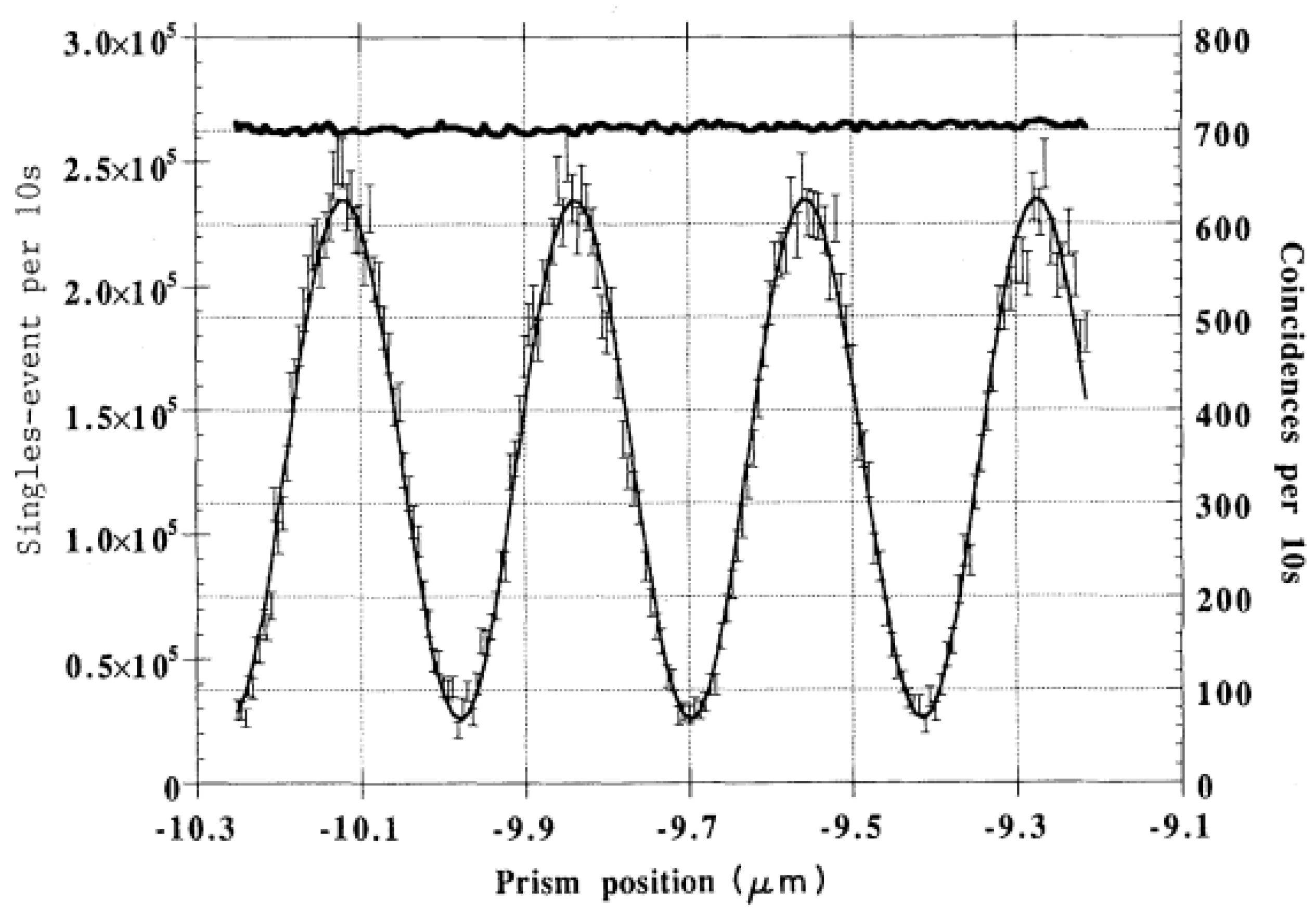
The other half corresponds to pairs for which both photons are detected simultaneously. If they are detected either by detectors $D_A$ and $D_B$ or by detectors $D_A^{\prime }$ and $D_B^{\prime }$, they are counted as event $\#1$. On the other hand, if they are detected either by detectors $D_A$ and $D_B^{\prime }$ or by detectors $D_A^{\prime }$ and $D_B$, they are counted as event $\#2$. As shown in Figure 3, which has been taken and reproduced here from reference [17], these events occur with probabilities that show a characteristic pattern of interference fringes as a function of the length difference $\mathsf{\Delta }L$ introduced in the experimental setting (9), even though the total number of photons collected at each one of the four detectors do not show any such fringes, which is in good agreement with the predictions (4) of quantum mechanics.

As it can be seen from Figure 3 and Equation (11), the period of the interference pattern in these probabilities is fixed by the wavelength of the incident photon splitted via parametric downconversion at the non-linear crystal.

$$\mathit{l}\sim {\lambda }_p\sim 0.35\mathsf{\mu }\mathrm{m}.$$

(12)

The described interference pattern in the probabilities of simultaneous events is attributed within the framework of quantum mechanics to the experimental impossibility to distinguish if the pair of simultaneous photons arrived at their detectors either both through the longer arms or both through the shorter arms of their respective interferometers. The two possibilities are undistinguishable because, as we observed above in Equation (8), the uncertainty in their emission time caused by the time width of the laser pulse, $T\sim 20\mathrm{ns}$, is much longer than the time delay introduced by the length difference between the longer and shorter arms, $\mathsf{\Delta }t\sim 2\mathrm{ns}$ [14,15,17].

4. The Statistical Model

In this section, we describe an explicit model of local hidden variables that reproduces the predictions of quantum mechanics for the ideal Franson experiment, as summarized in Equation (4). The model closely resembles the model introduced in [8,9,10] to reproduce the predictions of quantum mechanics for the Bell experiment. It also bears some similarities as well as many crucial differences, which we highlight below, with the model of hidden variables introduced by Aerts et al. in [21]. The comparison between the two models will help us to make clear the novel features of our model.

The crux of our model is the spontaneous breaking of the time-translation gauge symmetry by the hidden configurations of the pair of photons produced in the non-linear crystal. The breaking of time-translation symmetry in this model is tantamount, as we show below, to the impossibility to set the time of emission of the photons with precision better than roughly $10\%$ of the period of the observed interference fringes (12), that is, ∼$0.03\mathsf{\mu }\mathrm{m}/\mathrm{c}\sim {10}^{-16}\mathrm{s}$. At the origin of this uncertainty is a geometric phase associated with a holonomy, as intuitively illustrated in Figure 3 in [8]. In the example shown in that figure, three parties located on the surface of a sphere cannot agree on the orientation of a tangent vector shared between them to a precision better than the geometric phase that the vector acquires when transported over the closed loop that connects the parties. In the model discussed in this paper, the three parties are the source of the pairs of photons and the detectors at both ends of the optical device, which cannot agree on the phase of the photons shared between them due to a similar holonomy.

Since the time uncertainty associated to this holonomy is shorter by three orders of magnitude than the coherence time of the two propagating photons, see

Table 1. Characteristic time and length scales in the Franson experiment reported in reference [17].

	Time Scale	Length Scale
Laser pulse	∼20 ns	∼6 m
Arms imbalance	∼2 ns	∼60 cm
Photons coherence	∼${10}^{-4}$ ns	∼36 $\mathsf{\mu }$m
Interference fringes	∼${10}^{-6}$ ns	∼0.3 $\mathsf{\mu }$m

, it cannot be discarded as a key ingredient for a succesful description within the framework of a model of local hidden variables of the pattern of inteference fringes observed in the Franson experiment. Nonetheless, Aerts et al. claim in [21] that “The emission time should be one of the (well-defined) variables, because if the beam splitters of, say, the right interferometer were removed, the photons would be detected solely by the detector $+1$, and the detection time $t_E$ would indicate the moment of emission”, thus discarding from their considerations the possibility of spontaneous breaking of the time translation symmetry and the appearance of a holonomy.

We consider a statistical model in which the space of possible hidden configurations of the pairs of photons consists of two separated sub-populations, each one of them occurring with a probability of one half. The first sub-population accounts for events in which the two photons of the pair are detected simultaneously, that is, events $\#1$ and $\#2$ in (4), for which their probabilities depend on the total phase defined by the setting of the experiment:

$$\mathsf{\Delta }\equiv {\varphi }_A+{\varphi }_B-\frac{\pi }{2}=2\pi \frac{{\omega }_p\mathsf{\Delta }L}{c}-\frac{\pi }{2},$$

(13)

while the second sub-population accounts for events in which the two photons of the pair are detected at distinct times, that is, events $\#3$ and $\#4$, for which their probabilities do not depend on the setting of the experiment.

The statistical space consists of an infinitely large number of possible hidden configurations distributed over the unit circle, with a density of probability given by the following:

$$g\left({\phi }_A\right)=\frac{1}{4}\left|sin\left({\phi }_A\right)\right|,$$

(14)

where ${\phi }_A\in [-\pi ,\pi )$ is an angular coordinate over the circle, i.e., a phase, which determines if photon A will be detected either at detector $D_A$ or at detector $D_A^{\prime }$, according to the following.

$$\begin{array}{c}\hfill {\mathcal{S}}^{\left(A\right)}=\mathcal{S}\left({\phi }_A\right)=\left\{\begin{array}{cccc}{D}_A,& if& {\phi }_A\in & [-\pi ,0)\\ D_A^{\prime },& if& {\phi }_A\in & [0,+\pi )\end{array}\right.\end{array}$$

(15)

Since $g\left({\phi }_A\right)=g(-{\phi }_A)$, each one of the two possibilities occurs with a probability of one half. Let us notice that the density of probability (14) is normalized to the following.

$${\int }_{-\pi }^{+\pi }d{\phi }_{A}g\left({\phi }_A\right)=1.$$

(16)

This coordinate is somewhat similar to the angular coordinate $\theta$ used in the model of hidden variables built by Aerts et al. in [21]. In their model the random variable $\theta$ is distributed uniformly over its range $[-\pi ,\pi )$, but they introduce a non-uniform boundary to produce the correct distribution.

Each one of these possible hidden configurations may appear in four possible shapes, labelled as $({\eta }_A=\pm 1,{\eta }_B=\pm 1)$, each one with a probability of $1/4$. These shapes determine if the photons are detected either at the earlier or the later time slot according to the following:

$$\begin{array}{c}\hfill {\mathit{s}}^{\left(N\right)}=\left\{\begin{array}{ccc}\mathrm{EARLY},& \mathrm{if}& {\eta }_N=-1\\ \mathrm{LATE},& \mathrm{if}& {\eta }_N=+1\end{array}\right.,\end{array}$$

(17)

where $N=A,B$. For example, photon A of a pair with shape defined by ${\eta }_A=+1,{\eta }_B=-1$ will be detected in the later time slot, while photon B of the same pair will be detected at the earlier time slot. These binary variables come instead the continuous coordinate $r\in [0,1]$ considered in the model discussed by Aerts et al. in [21].

In simultaneous events, the two photons of the pair acquire equal phases ${\varphi }_A={\varphi }_B=\pi {\omega }_p\mathsf{\Delta }L/c$ as they go through their respective interferometers, which add up to a total phase that depends on the setting of the experiment (13):

$$\tilde{\mathsf{\Delta }}={\eta }_A·\mathsf{\Delta }={\eta }_A·\left({\varphi }_A+{\varphi }_B-\frac{\pi }{2}\right),\mathrm{if}{\eta }_A={\eta }_B,$$

(18)

while in not-simultaneous events the two photons acquire opposite phases ${\varphi }_A=-{\varphi }_B$ so that the total phase between the two does not depend on the experimental setting.

$$\tilde{\mathsf{\Delta }}=-{\eta }_A·\frac{\pi }{2},\mathrm{if}{\eta }_A=-{\eta }_B.$$

(19)

A hidden configuration characterized by a phase ${\phi }_A$ at the exit of interferometer A is described at the exit of interferometer B by a phase ${\phi }_B$ related to the former by the following coordinate transformation:

$${\phi }_B=L({\phi }_A,\tilde{\mathsf{\Delta }}),$$

(20)

where the transformation function is defined as follows:

• If $\tilde{\mathsf{\Delta }}\in [0,\pi )$, then we have the following:

  $$\begin{array}{c}\hfill L(\phi ;\tilde{\mathsf{\Delta }})=\left\{\begin{array}{c}q\left(\phi \right)·\mathrm{arc}-\cos \left(-cos\left(\tilde{\mathsf{\Delta }}\right)-cos\left(\phi \right)-1\right),\\ \mathrm{if}-\pi \le \phi <\tilde{\mathsf{\Delta }}-\pi ,\\ q\left(\phi \right)·\mathrm{arc}-\cos \left(+cos\left(\tilde{\mathsf{\Delta }}\right)+cos\left(\phi \right)-1\right),\\ \mathrm{if}\tilde{\mathsf{\Delta }}-\pi \le \phi <0,\\ q\left(\phi \right)·\mathrm{arc}-\cos \left(+cos\left(\tilde{\mathsf{\Delta }}\right)-cos\left(\phi \right)+1\right),\\ \mathrm{if}0\le \phi <\tilde{\mathsf{\Delta }},\\ q\left(\phi \right)·\mathrm{arc}-\cos \left(-cos\left(\tilde{\mathsf{\Delta }}\right)+cos\left(\phi \right)+1\right),\\ \mathrm{if}\tilde{\mathsf{\Delta }}\le \phi <+\pi ,\end{array}\right.\end{array}$$

  (21)
• If $\tilde{\mathsf{\Delta }}\in [-\pi ,0)$, then we have the following:

  $$\begin{array}{c}\hfill L(\phi ;\tilde{\mathsf{\Delta }})=\left\{\begin{array}{c}q\left(\phi \right)·\mathrm{arc}-\cos \left(-cos\left(\tilde{\mathsf{\Delta }}\right)+cos\left(\phi \right)+1\right),\\ \mathrm{if}-\pi \le \phi <\tilde{\mathsf{\Delta }},\\ q\left(\phi \right)·\mathrm{arc}-\cos \left(+cos\left(\tilde{\mathsf{\Delta }}\right)-cos\left(\phi \right)+1\right),\\ \mathrm{if}\tilde{\mathsf{\Delta }}\le \phi <0,\\ q\left(\phi \right)·\mathrm{arc}-\cos \left(+cos\left(\tilde{\mathsf{\Delta }}\right)+cos\left(\phi \right)-1\right),\\ \mathrm{if}0\le \phi <\tilde{\mathsf{\Delta }}+\pi ,\\ q\left(\phi \right)·\mathrm{arc}-\cos \left(-cos\left(\tilde{\mathsf{\Delta }}\right)-cos\left(\phi \right)-1\right),\\ \mathrm{if}\tilde{\mathsf{\Delta }}+\pi \le \phi <+\pi ,\end{array}\right.\end{array}$$

  (22)

where we have made use of the function:

$$\begin{array}{c}\hfill q\left(\phi \right)=\mathrm{sign}\left((\phi -\tilde{\mathsf{\Delta }})\mathrm{mod}\left([-\pi ,\pi )\right)\right),\end{array}$$

and defined the function $y=\mathrm{arc}-\cos \left(x\right)$ in its main branch, such that $y\in [0,\pi ]$ while $x\in [-1,+1]$.

We have shown in [8,9,10] that this coordinates transformation fulfills the following constraint:

$$d{\phi }_{A}g\left({\phi }_A\right)=d{\phi }_{B}g\left({\phi }_B\right),$$

(23)

so that the phases ${\phi }_B$ are distributed over the circle with a density of probability:

$$g\left({\phi }_B\right)=\frac{1}{4}\left|sin\left({\phi }_B\right)\right|$$

(24)

that is functionally identical to the density of probability for the phases ${\phi }_A$, as it should be expected from symmetry considerations. Furthermore, constraint (23) states that the probability to occur of each possible configuration is independent—as it must be—from the set of coordinates used to describe them.

In order to keep the symmetry between the two involved parties, we stipulate that photon B is detected either at detector $D_B$ or at detector $D_B^{\prime }$ according to the same response function defined above for photon A.

$$\begin{array}{c}\hfill {\mathcal{S}}^{\left(B\right)}=\mathcal{S}\left({\phi }_B\right)=\left\{\begin{array}{cccc}{D}_B,& \mathrm{if}& {\phi }_B\in & [-\pi ,0)\\ D_B^{\prime },& \mathrm{if}& {\phi }_B\in & [0,+\pi )\end{array}\right.\end{array}$$

(25)

Therefore, for simultaneous events, we have the following:

$$\begin{array}{ccc}\hfill p_1=p\left[\left(D_A\bigcap D_B\right)\bigcup \left(D_A^{\prime }\bigcap D_B^{\prime }\right)\right]& =& \frac{1}{4}\left[1+cos\left(\tilde{\mathsf{\Delta }}\right)\right],\hfill \\ \hfill p_2=p\left[\left(D_A^{\prime }\bigcap D_B\right)\bigcup \left(D_A\bigcap D_B^{\prime }\right)\right]& =& \frac{1}{4}\left[1-cos\left(\tilde{\mathsf{\Delta }}\right)\right],\hfill \end{array}$$

which exactly reproduces the probabilities (4) for events $\#1$ and $\#2$. For non-simultaneous events, on the other hand, we obtain the following:

$$\begin{array}{ccc}\hfill p_3=p\left[\left(D_A\bigcap D_B\right)\bigcup \left(D_A^{\prime }\bigcap D_B^{\prime }\right)\right]& =& \frac{1}{4},\hfill \\ \hfill p_4=p\left[\left(D_A^{\prime }\bigcap D_B\right)\bigcup \left(D_A\bigcap D_B^{\prime }\right)\right]& =& \frac{1}{4},\hfill \end{array}$$

which also corresponds to the probabilities (4) for events $\#3$ and $\#4$.

In order to obtain these results, we notice that $L({\phi }_A;\tilde{\mathsf{\Delta }})$ changes signs at ${\phi }_A=\tilde{\mathsf{\Delta }}$ and at ${\phi }_A=\tilde{\mathsf{\Delta }}-\pi$ (see Figure 4); therefore, we have the following.

$$\begin{array}{ccc}\hfill p\left[\left(D_A\bigcap D_B\right)\bigcup \left(D_A^{\prime }\bigcap D_B^{\prime }\right)\right]& =& {\int }_{\tilde{\mathsf{\Delta }}-\pi }^{0}d{\phi }_{A}g\left({\phi }_A\right)+{\int }_{\tilde{\mathsf{\Delta }}}^{\pi }d{\phi }_{A}g\left({\phi }_A\right),\hfill \end{array}$$

(26)

$$\begin{array}{ccc}\hfill p\left[\left(D_A^{\prime }\bigcap D_B\right)\bigcup \left(D_A\bigcap D_B^{\prime }\right)\right]& =& {\int }_{-\pi }^{\tilde{\mathsf{\Delta }}-\pi }d{\phi }_{A}g\left({\phi }_A\right)+{\int }_0^{\tilde{\mathsf{\Delta }}}d{\phi }_{A}g\left({\phi }_A\right).\hfill \end{array}$$

(27)

The coordinate transformation (20) as defined in (21) and (22) introduces the holonomy responsible for the time uncertainty mentioned above. This non-linear transformation generalizes the linear transformation ${\tilde{\phi }}_B={\phi }_A+\tilde{\mathsf{\Delta }}$ assumed as an unavoidable must in the model of hidden variables discussed by Aerts et al. in [21]. In Figure 4, the transformation (20) is plotted against the linear transformation for the particular value $\tilde{\mathsf{\Delta }}=\pi /3$ for the sake of illustration. The maximum difference between the actual transformation $L(\phi ;\tilde{\mathsf{\Delta }})$ and the linear transformation, which bounds the geometric phase that can be accumulated in a cycle, is roughly a $10\%$ of the period of the transformation, that is, ∼$0.1{\omega }_p^{-1}\sim {10}^{-16}s$.

As already observed, this model closely resembles the model of local hidden variables introduced in [8,9,10]. The crux of both models is the spontaneous breaking of a gauge symmetry by the hidden configuration of the described pairs of photons, which acquires a non-zero geometric phase through certain cyclic transformations. In the model discussed here, the spontaneously broken gauge symmetry is the time-translation symmetry or equivalently the rotational symmetry of the phases ${\phi }_A$, ${\phi }_B$ of the hidden configurations, which cannot be described at once with respect to the two splitters and the source of the photons due to the holonomy of the model.

In both cases, however, gauge symmetries are statistically restored when considered over the entire population of possible hidden configurations, in agreement with Elitzur’s theorem that forbids any gauge-dependent magnitude to obtain a non-invariant expected value [22]. Thus, in the model discussed in this paper, the expected probabilities (4) predicted by the model depend only on the well-defined physical parameter ${\varphi }_A+{\varphi }_B$ that describes the experimental setting.

5. Discussion

We have presented an explicit model of local hidden variables that reproduces the predictions of quantum mechanics for the Franson experiment with pairs of photons locked in time and energy produced by parametric down-conversion in a non-linear crystal [14,17]. The model resembles closely the model of hidden variables introduced in [8,9,10] to reproduce the predictions of quantum mechanics for the Bell experiment with pairs of photons prepared in a singlet polarization state.

The crux of both models is the spontaneous breaking of a gauge symmetry by the hidden configuration of the pairs of photons, which acquires a non-zero geometric phase through certain cyclic coordinates transformations. In the model presented in this paper the broken gauge symmetry is the time-translation symmetry. The symmetry is broken at the scale of $\sim {10}^{-16}s$, which is roughly the inverse of the frequency of the photon splitted via parametric down conversion and much shorter than the coherence time of each one of the photons of the resulting pair.

The insight described here for pairs of photons produced via parametric down-conversion at a non-linear crystal might also be applied to study pairs of photons (or Z-bosons) produced in the decay of scalar massive particles such as, for example, positronium or neutral pions [24].