An Active Set Limited Memory BFGS Algorithm for Machine Learning

Abstract

In this paper, a stochastic quasi-Newton algorithm for nonconvex stochastic optimization is presented. It is derived from a classical modified BFGS formula. The update formula can be extended to the framework of limited memory scheme. Numerical experiments on some problems in machine learning are given. The results show that the proposed algorithm has great prospects.

1. Introduction

Machine learning is an interdisciplinary subject involving probability theory, statistics, approximation theory, convex analysis, algorithm complexity theory, and so on. In machine learning, people usually construct an appropriate model from an extraordinary large amount of data. Therefore, the traditional algorithms for solving optimization problems are no longer suitable for machine learning problems. A stochastic algorithm must be used to solve the model optimization problem we encounter in machine learning.

This type of problem is considered in machine learning

$$\underset{x\in {\Re }^d}{min}f(x)=\mathbb{E}\left[T(x,\tau )\right],$$

(1)

where $T:{\Re }^{D_x}\times {\Re }^n\to \Re$ is a continuously differentiable function, $\mathbb{E}[·]$ denotes the expectation taken with respect $\tau$ and $\tau$ is the random variable of the distribution function $\mathbb{P}$. In most practical cases, the function $T(·,\tau )$ is not given intuitively. In addition, even worse, the distribution function $\mathbb{P}$ may also be unknown. The objective function (1) is defined using the empirical expectation

$$f(x)=\frac{1}{\mathbb{N}}\sum _{n=1}^{\mathbb{N}}{f}_i(x),$$

(2)

where $f_i:{\Re }^{D_x}\to \Re$ is the loss function that corresponds to the ith data sample, and $\mathbb{N}$ denotes the number of data samples which is assumed to be extremely large.

The stochastic approximation ($SA$) algorithm is usually used to solve the above problems by Robbins and Monro [1]. The original SA algorithm can also be called random gradient descent ($SGD$). It is somewhat similar to the classical steepest descent method, which adopts the iterative process of $x_{k+1}=x_k-{\alpha }_k{g}_k$. In general, random gradient $g_k$ is used to represent the approximation of the full gradient $\nabla f$ of f at $x_k$ and ${\alpha }_k$ is the step size (Learning rate). The SA algorithm has been deeply studied by many scholars [2,3,4].

In this thesis, we mainly study the stochastic second-order method, that is, stochastic quasi-Newton methods $(SQN)$ to solve problem (2). Among the traditional optimization methods, the quasi-Newton methods have faster convergence speed and higher convergence accuracy than the first-order method because it uses the approximate second-order derivative information. The quasi Newton method is usually updated by the following iterative formula:

$$x_{k+1}=x_k-{\alpha }_k{B}_k^{-1}\nabla f(x)or{x}_{k+1}=x_k-{\alpha }_k{H}_k\nabla f(x)$$

(3)

where $B_k$ is the symmetric positive definite approximation of Hessian matrix ${\nabla }^{2}f(x)$ at $x_k$ or $H_k$ is the symmetric positive definite approximation of ${\left[{\nabla }^{2}f(x)\right]}^{-1}$. In the traditional BFGS algorithm, the iterative formula of $B_k$ is as follows:

$$B_k=B_{k-1}+\frac{y_{k-1}{y}_{k-1}^T}{s_{k-1}^T{s}_{k-1}}-\frac{B_{k-1}{s}_{k-1}{s}_{k-1}^T{B}_{k-1}}{s_{k-1}^T{B}_{k-1}{s}_{k-1}},$$

(4)

where $s_{k-1}=x_k-x_{k-1}={\alpha }_k{d}_k$ and $y_{k-1}=\nabla f(x_k)-\nabla f(x_{k-1})$. If formula Sherman–Morrison–Woodbury formula is used, the iterative formula of $H_k$ can be easily obtained:

$$H_k=(I-\frac{s_{k-1}{y}_{k-1}^T}{s_{k-1}^T{y}_{k-1}})H_{k-1}(I-\frac{s_{k-1}{y}_{k-1}^T}{s_{k-1}^T{y}_{k-1}})+\frac{s_{k-1}{s}_{k-1}^T}{s_{k-1}^T{y}_{k-1}}.$$

(5)

It is very important to use a limited memory variant for large-scale problems. This so-called L-BFGS [5] algorithm has a linear convergence rate. It produces well scaled and productive search directions that yield an approximate solution in fewer iterations and function evaluations. In stochastic optimization, many stochastic quasi Newton formulas have been proposed.

The LBFGS method has the following iteration rule $x_{k+1}=x_k-{\alpha }_k{H}_k\nabla f(x)$. The LBFGS method updates $H_k$ by the following rule:

$$\begin{array}{cc}\hfill H_k& =Q_{k-1}^T{H}_{k-1}{Q}_{k-1}+{\rho }_{k-1}{s}_{k-1}{s}_{k-1}^T\hfill \\ & =Q_{k-1}^T[Q_{k-2}^T{H}_{k-2}{Q}_{k-2}+{\rho }_{k-2}{s}_{k-2}{s}_{k-2}^T]Q_{k-1}+{\rho }_{k-1}{s}_{k-1}{s}_{k-1}^T\hfill \\ \hfill & =\dots \hfill \\ \hfill & =[Q_{k-1}^T\dots Q_{k-r+1}^T]H_{k-r+1}[Q_{k-r+1}^T\dots Q_{k-1}^T]\hfill \\ & +{\rho }_{k-r+1}[Q_{k-2}^T\dots Q_{k-r+2}^T]s_{k-r+1}{s}_{k-r+1}^T[Q_{k-r+2}^T\dots Q_{k-2}^T]\hfill \\ \hfill & +\dots +{\rho }_{k-1}{s}_{k-1}{s}_{k-1}^T,\hfill \end{array}$$

(6)

where $Q_{k-1}=I-{\rho }_{k-1}{y}_{k-1}{s}_{k-1}^T$, ${\rho }_{k-1}=\frac{1}{s_{k-1}^T{y}_{k-1}}$ and r is the memory size. Bordes, Bottomu, and Gallinari studied the quasi Newton method of diagonal rescaling matrix based on secant in [6]. In [7], Byrd et al. proposed a stochastic LBFGS method based on SA and proved its convergence for strongly convex problems. In [8], Gower, Goldfarb, and Richtárik proposed a variance reduced block L-BFGS method that converges linearly for convex functions. It is worth noting that, in the above quasi-Newton methods, the convergence of the algorithm needs to be convex or strongly convex.

If the objective function itself does not have the property of convexity, there are several problems that the LBFGS method has difficulty overcoming:

• How can we guarantee the positive definiteness of iterative matrix $H_k$ without line search?
• How can we guarantee the convergence of the proposed L-BFGS method?

These problems seem particularly difficult. However, a modified stochastic limited BFGS (LMLBFGS) is proposed to solve the above problems. On this basis, a new improved algorithm (LMLBFGS-VR) is proposed. Note that our presented algorithm can be adapted to approximate the solution of a nonlinear system of equations in [9].

This paper is divided into five parts: in Section 2, the LMLBFGS and LMLBFGS-VR are presented and their convergence properties are discussed in Section 3. In Section 4, the numerical experiments of the proposed algorithm are given. A summary is given in the last part.

2. Premise Setting and Algorithm

In this part, a new LBFGS(LMLBFGS) algorithm is proposed, which can automatically generate a positive definite matrix $B_k$.

2.1. LMLBFGS Algorithm

In order to solve this kind of problem, suppose that $\mathcal{E}\subset {\Re }^n$ does not depend on x and the random gradient $g(x,\tau )$ at x is generated by a stochastic first-order oracle (SFO), for which the distribution of $\tau$ is supported on $\mathcal{E}\subset {\Re }^n$. It is common to use a mini-batch stochastic gradient of the i-th sampling during the k-th iteration, which is described as

$$g_k=\frac{1}{z_k}\sum _{i\in Z_k}g(x_k,{\tau }_{k,i})=\frac{1}{z_k}\sum _{i\in Z_k}\nabla f_i(x_k),$$

(7)

and a sub-sampled Hessian defined as follows

$$G_k=\frac{1}{z_k^{*}}\sum _{i\in Z_k^{*}}G(x_k,{\tau }_{k,i})=\frac{1}{z_k^{*}}\sum _{i\in Z_k^{*}}{\nabla }^2{f}_i(x_k).$$

(8)

We have the subset $Z_k$ and $Z_k^{*}$ is the sample number where $z_k$ and $z_k^{*}$ are the cardinalities of $Z_k$ and $Z_k^{*}$. ${\tau }_{k,i}$ is a random variable. From the definition of random gradient, it is not difficult to find that the random gradient under this setting can be calculated faster than the full gradient. We assume here that the SFO generation method can separate $x_k$ and ${\tau }_k$ independently and generate the output $g(x_k,{\tau }_{k,i})$. Therefore, the stochastic gradient difference and the iterative difference are defined as

$$y_k=g_k-g_{k-1}=\frac{1}{z_k}\sum _{i\in Z_k}g(x_k,{\tau }_{k,i})-\frac{1}{z_{k-1}}\sum _{i\in Z_{k-1}}g(x_{k-1},{\tau }_{k-1,i}),$$

(9)

$$s_k=x_k-x_{k-1}.$$

(10)

In traditional methods, the authors in [10] proposed a new type of $\overline{y_k}$ by using

$$\overline{y_k}=y_k+{\lambda }_k{s}_k,$$

(11)

where

$${\lambda }_k=\frac{2[f(x_{k-1})-f(x_k)]+{(g_k+g_{k-1})}^T{s}_k}{{(s_k^T{y}_k)}^2}·(y_k{y}_k^T).$$

(12)

Inspired by their methods, we have the following new definitions:

$$y_k^{*}=y_k+{\lambda }_k{s}_k,$$

(13)

where

$${\lambda }_k=\frac{2[f(x_{k-1})-f(x_k)]+{(g_k+g_{k-1})}^T{s}_k}{max\left\{{(s_k^T{y}_k)}^2,{\parallel s_k\parallel }^4\right\}}·(y_k{y}_k^T).$$

(14)

Our ${\lambda }_k$ is guaranteed to be meaningful by $max\left\{{(s_k^T{y}_k)}^2,{\parallel s_k\parallel }^4\right\}>0.$

Hence, our stochastic LBFGS algorithm updates $B_k$ is

$$B_k=B_{k-1}+\frac{y_{k-1}^{*}{y}_{k-1}^{*T}}{s_{k-1}^T{s}_{k-1}}-\frac{B_{k-1}{s}_{k-1}{s}_{k-1}^T{B}_{k-1}}{s_{k-1}^T{B}_{k-1}{s}_{k-1}}.$$

(15)

Using the Sherman–Morrison–Woodbury formula, we can update $H_k=B_k^{-1}$ as

$$H_k=(I-\frac{s_{k-1}{y}_{k-1}^T}{s_{k-1}^T{y}_{k-1}})H_{k-1}(I-\frac{s_{k-1}{y}_{k-1}^T}{s_{k-1}^T{y}_{k-1}})+\frac{s_{k-1}{s}_{k-1}^T}{s_{k-1}^T{y}_{k-1}}.$$

(16)

Through simple observation, we can find the fact that, when the function is nonconvex, we can not guarantee that $s_k^T{y}_k^{*}>0$ is true. Thus, we add some additional settings to the algorithm to ensure the nonnegativity of $s_k^T{y}_k^{*}$. Define the index set $\mathcal{K}$ as follows:

$$\mathcal{K}=\{i:s_k^T{y}_k^{*}\ge m\parallel s_k{\parallel }^2\},$$

(17)

where m is a positive constant.

Hence, our modified stochastic L-BFGS algorithm updates (18) and (19):

$$B_k=\left\{\begin{array}{c}{B}_{k-1}+\frac{y_{k-1}^{*}{y}_{k-1}^{*T}}{s_{k-1}^T{s}_{k-1}}-\frac{B_{k-1}{s}_{k-1}{s}_{k-1}^T{B}_{k-1}}{s_{k-1}^T{B}_{k-1}{s}_{k-1}},ifk\in K,\\ B_{k-1},otherwise,\end{array}\right.$$

(18)

$$H_k=\left\{\begin{array}{c}{H}_k=(I-\frac{s_{k-1}{y}_{k-1}^T}{s_{k-1}^T{y}_{k-1}})H_{k-1}(I-\frac{s_{k-1}{y}_{k-1}^T}{s_{k-1}^T{y}_{k-1}})+\frac{s_{k-1}{s}_{k-1}^T}{s_{k-1}^T{y}_{k-1}},ifk\in K\\ H_{k-1},otherwise.\end{array}\right.$$

(19)

As is known to all, the cost of calculating $H_k$ through (19) is very huge when n is tremendously large. Hence, the LBFGS method is usually used instead of the BFGS method to overcome the poser of a large amount of calculation in large-scale optimization problems. The advantage of LBFGS is that it only uses curvature information and does not need to store the update matrix, which can effectively reduce the computational cost: Use (6) to iterate

$$H_{k,i}=(I-{\rho }_j{s}_j{y}_j^{*T})H_{k,i-1}(I-{\rho }_j{y}_j^{*}{s}_j^T)+{\rho }_j{s}_j{s}_j^T,j=k-(r-i);i=0,\dots ,r-1,$$

(20)

where ${\rho }_j=1/(s_j^T{y}_j^{*})$. The initial matrix is often chosen as: $H_{k,0}=\frac{s_{k-1}^T{y}_{k-1}^{*}}{y_{k-1}^{*T}}I$. Because $s_{k-1}^T{y}_{k-1}^{*}$ may be exceedingly close to 0, we set

$$H_{k,0}={\gamma }_k^{-1}I,$$

(21)

and

$${\gamma }_k=max\{\frac{\parallel y_{k-1}^{*}\parallel }{s_{k-1}^T{y}_{k-1}^{*}},\delta \}\ge \delta ,$$

(22)

where $\delta$ is a given constant.

Therefore, our modified stochastic L-BFGS algorithm is outlined in Algorithm 1.

Algorithm 1: Modified stochastic LBFGS algorithm (LMLBFGS).

Input: Given $x_1\in {\Re }^n$, batch size $z_k$, ${\alpha }_k$, the memory size r, a positive definite matrix $H_1$, and a positive constant $\delta$   1: for $k=0,1,\dots ,$ do   2:    Compute $g_k$ by (7) and Hessian matrix $H_k$ by Algorithm 2;   3:    Compute the iteration point $x_{k+1}=x_k-{\alpha }_k{H}_k{g}_k$.   4: end for

2.2. Extension of Our LMLBFGS Algorithm with Variance Reduction

Recently, using variance reduction technology in stochastic optimization methods can make the algorithm have better properties. Motivated by the development of the SVRG method for nonconvex problems, we present a new modified stochastic LBFGS algorithm (called LMLBFGS-VR) with a variance reduction technique for a faster convergence speed, as shown in Algorithm 3.

In LMLBFGS-VR, the mini-batch stochastic gradient is defined as

$$g(x)=\frac{1}{\left|\mathcal{Z}\right|}\sum _{i\in \mathcal{Z}}\nabla f_i(x),\mathcal{Z}\subset \{1,2,\dots ,n\}.$$

(23)

Algorithm 2: Hessian matrix updating.

Input: correction pairs $(s_j,y_j)$, memory parameter r, and $j=k-(r-i);i=0,\dots ,r-1,$ Output: new $H_k$   1: $H=\frac{s_k^T{y}_k^{*}}{y_t^{*T}{y}_t^{*}}I$   2: for $j=k-(r-i);i=0,\dots ,r-1$ do   3:     $m_j=s_j^T{y}_j^{*}-m{\parallel s_j\parallel }^2,{\rho }_j=\frac{1}{s_j^T{y}_j^{*}}$   4:     if $\mathbf{then}{m}_j>0$   5:         $H=(I-s_j{y}_j^{*T}{\rho }_j)H(I-y_j^{*}{s}_j^T{\rho }_j)+{\rho }_j{s}_j{s}_j^T$   6:     end if   7: end for   8: return $H_k=H$

Algorithm 3: Modified stochastic LBFGS algorithm with variance reduction (LMLBFGS-VR).

Input: Given ${\overline{x}}_0\in {\Re }^n$, $H_0=I$, batch size $z_k$, ${\alpha }_k$, the memory size r and a constant $\delta >0$ Output: Iterationxis chosen randomly from a uniform $\{l_u^{k+1}:u=0,\dots ,q-1;$$k=0,\dots ,N-1\}$   1: for $k=0,1,\dots ,N-1$ do   2:     $l_0^{k+1}={\tilde{x}}_k$   3:     compute $\nabla f({\overline{x}}_k)$   4:     for $u=0,1,\dots ,q-1$ do   5:         Samlple a minibatch $\mathcal{Z}$ with $\left|\mathcal{Z}\right|=|Z_k|$   6:         Calculate $g_u^{k+1}=\nabla f_{\mathcal{Z}}(l_u^{k+1})-\nabla f_{\mathcal{Z}}({\overline{x}}_k)+\nabla f({\overline{x}}_k)$ where $\nabla f_{\mathcal{Z}}(l_u^{k+1})=\frac{1}{\left|\mathcal{Z}\right|}{\sum }_{i\in \mathcal{Z}}\nabla f_i(l_u^{k+1})$;   7:         Compute $l_{u+1}^{k+1}=l_u^{k+1}-{\alpha }_k{H}^{k+1}{g}_u^{k+1}$;   8:     end for   9:     Generate the updated Hessian matrix $H^{k+1}$ by Algorithm 2;   10:     ${\overline{x}}_{k+1}=l_q^{k+1}$   11: end for

3. Global Convergence Analysis

In this section, the convergence of Algorithms 1 and 3 will be discussed and analyzed.

3.1. Basic Assumptions

In the algorithm, it is assumed that the step size satisfies

$$\sum _{k=1}^{+\infty }{\alpha }_k=+\infty ,\sum _{k=1}^{+\infty }{\alpha }_k<+\infty .$$

(24)

Assumption 1.

$f:{\Re }^{D_x}\to \Re$ is continuously differentiable and for any $x\in {\Re }^n$, $f(x)$ is bounded below. This means that there is constant $L>0$ that makes

$$\parallel \nabla f(l_1)-\nabla f(l_2)\parallel \le L\parallel l_1-l_2\parallel$$

(25)

for any $l_1,l_2\in {\Re }^n$.

Assumption 2.

The noise level of the gradient estimation σ such that

$${\mathbb{E}}_{{\tau }_k}\left[g(x_k,{\tau }_k)\right]=\nabla f(x_k),$$

(26)

$${\mathbb{E}}_{{\tau }_k}[\parallel g(x_k,{\tau }_k)-\nabla f(x_k){\parallel }^2]\le {\sigma }^2,$$

(27)

where $\sigma >0$ and ${\mathbb{E}}_{{\tau }_k}[·]$ denotes the expectation taken with respect to ${\tau }_k$.

Assumption 3.

There are positive $h_1$ and $h_2$ such that

$$h_{1}I⪯H_k⪯h_{2}I.$$

(28)

Our random variables ${\tau }_k$ are defined as follows: ${\tau }_k=({\tau }_{k,1},\dots ,{\tau }_{k,z_k})$ are the random samplings in the k-th iteration, and ${\tau }_{\left[k\right]}=({\tau }_1,\dots ,{\tau }_k)$ are the random samplings in the first k-th iterations.

Assumption 4.

For any $k\ge 2$, the random variable $H_k$ depends only on ${\tau }_{\left[k-1\right]}$.

From (2) and (4), we can get

$$\mathbb{E}\left[H_k{g}_k\right|{\tau }_{\left[k\right]}]=H_k{g}_k.$$

(29)

3.2. Key Propositions, Lemmas, and Theorem

Lemma 1.

If Assumptions 1–4 hold and ${\alpha }_k\le \frac{h_1}{L{h}_2^2}$ for all k, we have

$$\mathbb{E}\left[f(x_{k+1})\right|x_k]\le -\frac{1}{2}{\alpha }_k{h}_1{\parallel \nabla f(x_k)\parallel }^2+f(x_k)+\frac{L{\sigma }^2{h}_2^2}{2z_k}{\alpha }_k^2,$$

(30)

where the conditional expectation is taken with respect to ${\tau }_k$.

Proof. 

$$\begin{array}{cc}\hfill f(x_{k+1})& \le f(x_k)+⟨\nabla f(x_k),x_{k+1}-x_k⟩+\frac{L}{2}\parallel x_{k+1}-x_k\parallel \hfill \\ \hfill & =f(x_k)-{\alpha }_k⟨\nabla f(x_k),H_k{g}_k⟩+\frac{L{\alpha }_k^2}{2}{\parallel H_k{g}_k\parallel }^2\hfill \\ \hfill & \le f(x_k)-{\alpha }_k⟨\nabla f(x_k),H_k\nabla f(x_k)⟩-{\alpha }_k⟨\nabla f(x_k),H_k(g_k-\nabla f(x_k))⟩\hfill \\ \hfill & +\frac{L{\alpha }_k^2{h}_2^2}{2}{\parallel g_k\parallel }^2.\hfill \end{array}$$

(31)

Taking expectation with respect to ${\tau }_k$ on both sides of (31) conditioned on $x_k$, we gain

$$\mathbb{E}\left[f(x_{k+1})\right|x_k]\le f(x_k)-{\alpha }_k⟨\nabla f(x_k),H_k\nabla f(x_k)⟩+\frac{L{\alpha }_k^2{h}_2^2}{2}\mathbb{E}[\parallel g_k{\parallel }^2\left|x_k\right],$$

(32)

where we use the fact that $\mathbb{E}\left[(g_k-\nabla f(x_k))\right|x_k]=0$. From Assumption 2, it follows that

$$\begin{array}{cc}\hfill \mathbb{E}[\parallel g_k{\parallel }^2|x_k]& =\mathbb{E}[\parallel g_k-\nabla f(x_k)+\nabla f(x_k){\parallel }^2|x_k]\hfill \\ \hfill & =\mathbb{E}[\parallel \nabla f(x_k){\parallel }^2|x_k]+2\mathbb{E}[\parallel g_k-\nabla f(x_k)\parallel |x_k]+\mathbb{E}[\parallel g_k-\nabla f(x_k){\parallel }^2\left|x_k\right]\hfill \\ \hfill & =\mathbb{E}[\parallel \nabla f(x_k){\parallel }^2|x_k]+\mathbb{E}[\parallel g_k-\nabla f(x_k){\parallel }^2\left|x_k\right]\hfill \\ \hfill & \le \parallel \nabla f(x_k){\parallel }^2+\frac{{\sigma }^2}{z_k}.\hfill \end{array}$$

Together with (32), we have

$$\mathbb{E}\left[f(x_{k+1})\right|x_k]\le f(x_k)-({\alpha }_k{h}_1-\frac{L}{2}{\alpha }_k^2{h}_2^2){\parallel \nabla f(x_k)\parallel }^2+\frac{L{\sigma }^2{h}_2^2}{2z_k}{\alpha }_k^2.$$

(33)

Then, combining that with ${\alpha }_k\le \frac{h_1}{L{h}_2^2}$ implies (30). □

Before proceeding further, the definition of supermartingale will be introduced [11].

Definition 1.

Let $\left\{{\mathcal{L}}_k\right\}$ be an increasing sequence of σ-algebras. If $\left\{W_k\right\}$ is a stochastic process satisfying

(1) 

$C\left[\right|W_k\left|\right]<\infty$,

(2) 

$W_k\in {\mathcal{L}}_k$and$\mathbb{E}\left[W_{k+1}\right|{\mathcal{L}}_k]\le W_k$, for all k,

then $\left\{W_k\right\}$ is called a supermartingale.

Proposition 1.

If $\left\{W_k\right\}$ is a nonnegative supermartingale, then ${lim}_{k\to \infty }{W}_k\to W$ almost surely and $\mathbb{E}\left[W\right]\le \mathbb{E}\left[W_0\right].$

Lemma 2.

Let $\left\{x_k\right\}$ be generated by Algorithm 1, where the batch size $z_k=z,$ for all k. Then, there is a constant $M_0$ such that

$$\mathbb{E}\left[f(x_k)\right]\le M_0$$

(34)

for all k.

Proof. 

For convenience of explanation, we have the following definitions:

$$w_k=\frac{1}{2}{\alpha }_k{h}_1{\parallel \nabla f(x_k)\parallel }^2,{\psi }_k=f(x_k)+\frac{L{\sigma }^2{h}_2^2}{2z}\sum _{i=k}^{\infty }{\alpha }_i^2.$$

(35)

Let $\underline{f}$ be the the lower bound of the function and $W_k$ be the $\sigma$-algebra measuring $x_k$, $w_k$ and ${\psi }_k$. From the definition, we obtain

$$\begin{array}{cc}\hfill \mathbb{E}\left[{\psi }_{k+1}\right|W_k]& =\mathbb{E}\left[f(x_{k+1})\right|W_k]+\frac{L{\sigma }^2{h}_2^2}{2z}\sum _{i=k+1}^{\infty }{\alpha }_k^2\hfill \\ \hfill & \le f(x_k)-\frac{1}{2}{\alpha }_k{h}_1{\parallel \nabla f(x_k)\parallel }^2+\frac{L{\sigma }^2{h}_2}{2z}\sum _{i=k+1}^{\infty }{\alpha }_k^2\hfill \\ \hfill & ={\psi }_k-w_k.\hfill \end{array}$$

(36)

Hence, we obtain

$$\mathbb{E}[{\psi }_{k+1}-\underline{f}|W_k]\le {\psi }_k-w_k-\underline{f}.$$

As a result, we have

$$0\le \mathbb{E}[{\psi }_{k+1}-\underline{f}]\le {\psi }_1-\underline{f}<\infty .$$

 □

3.3. Global Convergence Theorem

In this part, we provide the convergence analysis of the proposed Algorithms 1 and 3.

Theorem 1.

Assume that Assumptions 1–4 hold for $\left\{x_k\right\}$ generated by Algorithm 1, where the batch size is $z_k=z$. The step size satisfies (24) and ${\alpha }_k\le \frac{h_1}{L{h}_2}$.Then, we have

$$\underset{k\to \infty }{lim}inf\mathbb{E}[\parallel \nabla f(x_k){\parallel }^2]=0withprobability1.$$

(37)

Proof. 

According to Definition 1, ${\psi }_k-\underline{f}$ is a supermartingale. Hence, there exists a $\psi$ such that ${lim}_{k\to \infty }$ with probability 1, and $\mathbb{E}\left[\psi \right]\le \mathbb{E}\left[{\psi }_1\right]$ (Proposition 1). Form (36), we have $\mathbb{E}\left[w_k\right]\le \mathbb{E}\left[{\psi }_k\right]-\mathbb{E}\left[{\psi }_{k+1}\right]$. Thus,

$$\mathbb{E}[\sum _{k=1}^{\infty }{w}_k]\le \sum _{k=1}^{\infty }(\mathbb{E}\left[{\psi }_k\right]-\mathbb{E}\left[{\psi }_{k+1}\right])\le \infty ,$$

(38)

which means that

$$\sum _{k=1}^{\infty }{w}_k=\frac{h_1}{2}\sum {\alpha }_k{\parallel \nabla f(x_k)\parallel }^2<+\infty withprobability1.$$

(39)

Since (24), it follows that (48) holds. □

Next, the convergence of the algorithm can be given.

Theorem 2.

If Assumptions A1, A2, and A4 hold for $\left\{x_k\right\}$ generated by Algorithm 1, where the batch size is $z_k=z$. The step size satisfies (24) and ${\alpha }_k\le \frac{h_1}{L{h}_2}$. Then, we have

$$\underset{k\to \infty }{lim}inf\mathbb{E}[\parallel \nabla f(x_k){\parallel }^2]=0withprobability1.$$

(40)

Proof. 

The proof will be established by contradiction, and the discussion is listed as follows.

According to the definition of $y_k^{*}$, we have

$$\begin{array}{cc}\hfill s_j^T{y}_j^{*}& =s_j^T{y}_j+\frac{2[f(x_{j-1})-f(x_j)]+{(g_j+g_{j-1})}^T{s}_j}{max\left\{{(s_j^T{y}_j)}^2,{\parallel s_j\parallel }^4\right\}}·(s_j^T{y}_j{y}_j^T{s}_j)\hfill \\ \hfill & \le s_j^T{y}_j+\frac{2[f(x_{j-1})-f(x_j)]+{(g_j+g_{j-1})}^T{s}_j}{{(s_j^T{y}_j)}^2}·(s_j^T{y}_j{y}_j^T{s}_j)\hfill \\ \hfill & =s_j^T{y}_j+2[f(x_{j-1})-f(x_j)]+{(g_j+g_{j-1})}^T{s}_j\hfill \\ \hfill & =s_j^T{y}_j-2g{(x_{j-1}+\theta (x_j-x_{j-1}))}^T{s}_j+{(g_j+g_{j-1})}^T{s}_j\hfill \\ \hfill & =2s_j^T(g_j-g(x_{j-1}+\theta (x_j-x_{j-1})))\hfill \\ \hfill & \le 2(1-\theta )L\parallel s_j\parallel \parallel (x_j-x_{j-1})\parallel \hfill \\ \hfill & =2(1-\theta )L\parallel s_j{\parallel }^2,\hfill \end{array}$$

where $\theta \in (0,1)$. It is easy to see that

$$m\parallel s_j{\parallel }^2\le s_j^T{y}_j^{*}\le \Lambda {\parallel s_j\parallel }^2,$$

(41)

where $\mathsf{\Lambda }$ is a positive constant.

According to the definition of $y_k^{*}$, we have

$$\begin{array}{cc}\hfill \parallel y_j^{*}\parallel & =\parallel y_j+\frac{2[f(x_{j-1})-f(x_j)]+{(g_j+g_{j-1})}^T{s}_j}{max\left\{{(s_j^T{y}_j)}^2,{\parallel s_j\parallel }^4\right\}}·(y_j{y}_j^T)·s_j\parallel \hfill \\ \hfill & \le \parallel y_j\parallel +|2[f(x_{j-1})-f(x_j)]+{(g_j+g_{j-1})}^T{s}_j|\parallel \frac{y_j{y}_j^T}{\parallel s_j{\parallel }^4}{s}_j\parallel \hfill \\ \hfill & \le \parallel y_j\parallel +|-2g{(x_{j-1}+\theta (x_j-x_{j-1}))}^T{s}_j+{(g_j+g_{j-1})}^T{s}_j|·\frac{\parallel y_j{y}_j^T\parallel }{\parallel s_j{\parallel }^4}\parallel s_j\parallel \hfill \\ \hfill & \le \parallel y_j\parallel +|(g_j-g{(x_{j-1}+\theta (x_j-x_{j-1}))}^T{s}_j\hfill \\ \hfill & +(g_{j-1}-g{(x_{j-1}+\theta (x_j-x_{j-1}))}^T{s}_j{(g_j+g_{j-1})}^T{s}_j|·\frac{\parallel y_j{y}_j^T\parallel }{\parallel s_j{\parallel }^3}\hfill \\ \hfill & \le L\parallel s_j\parallel +(L(1-\theta )\parallel s_j{\parallel }^2+L\theta \parallel s_j{\parallel }^2)·\frac{\parallel y_j\parallel \parallel y_j\parallel }{\parallel s_j{\parallel }^3}\hfill \\ \hfill & =2L\parallel s_j\parallel .\hfill \end{array}$$

(42)

From (41) and (42), we have

$$\lambda \le \frac{\parallel y_j^{*}{\parallel }^2}{s_j^T{y}_j^{*}}\le \frac{{(2L)}^2{\parallel s_j\parallel }^2}{\lambda \parallel s_j{\parallel }^2}=\frac{{(2L)}^2}{\lambda }=M_0,$$

(43)

where the first inequality is derived from the quasi Newton condition. This equation shows that the eigenvalue of our initial matrix $B_k^{\left(0\right)}=\frac{y_k^{*T}{y}_k^{*}}{s_k^T{y}_k^{*}}I$ is bounded, and the eigenvalue is much greater than 0.

Instead of directly analyzing the properties of $H_k$, we get the results by analyzing the properties of $B_k$. In this situation, the limited memory quasi-Newton updating formula is as follows:

(i)

$B_k^{(0)}=\frac{y_k^{*T}{y}_k^{*}}{s_k^T{y}_k^{*}}I$.

(ii)

for $i=0,\dots ,r-1$, $j=k-(r-i)$ and

$$B_k^{\left(i+1\right)}=B_k^{\left(i\right)}-\frac{B_k^{\left(i\right)}{s}_j{s}_j^T{B}_k^{\left(i\right)}}{s_j^T{B}_k^{\left(i\right)}{s}_j}+{\displaystyle \frac{y_j^{*}{y}_j^{*T}}{s_j^T{y}_j^{*}}}.$$

(44)

The trace of matrix B is defined as $tr(B)$. Then, from (43) and (44), and the boundedness of $\{\parallel B_k^{\left(0\right)}\parallel \}$, we obtain

$$\begin{array}{cc}\hfill tr(B_{k+1})& \le tr(B_k^{\left(0\right)})+\sum _{i=1}^r\frac{\parallel y_j^{*}{\parallel }^2}{s_j^T{y}_j^{*}}\hfill \\ \hfill & \le tr(B_k^{\left(0\right)})+r\mathsf{\Lambda }\hfill \\ \hfill & =M_1.\hfill \end{array}$$

(45)

The determinant of $B_k$ is now considered because the determinant can be used to prove that the minimum eigenvalue of matrix B is uniformly bounded. From the theory in [12], we can get the following equation about matrix determinant:

$$\begin{array}{cc}\hfill det(B_{k+1})& =det(B_k^{\left(0\right)})\prod _{i=1}^r\frac{y_{j_i}^{*T}{s}_{j_i}}{s_{j_i}^T{B}_k^{\left(i-1\right)}{s}_{j_i}}\hfill \\ \hfill & =det(B_k^{\left(0\right)})\prod _{i=1}^r\frac{y_{j_i}^{*T}{s}_{j_i}}{s_{j_i}^T{s}_{j_i}}\frac{s_{j_i}^T{s}_{j_i}}{s_{j_i}^T{B}_k^{\left(i-1\right)}{s}_{j_i}}.\hfill \end{array}$$

(46)

It can be obtained from (45) that the maximum eigenvalue of matrix $B_j$ is uniformly bounded. Therefore, according to (41) and combining the fact that the smallest eigenvalue of $B_k^{\left(0\right)}$ is bounded away from zero, the following equation is obtained:

$$\begin{array}{cc}\hfill det(B_{k+1})& \ge det(B_k^{\left(0\right)}){(\frac{\lambda }{M_1})}^r\hfill \\ \hfill & \ge M_2.\hfill \end{array}$$

In this way, the maximum eigenvalue and the minimum eigenvalue of matrix $B_j$ are uniformly bounded and much greater than 0. Therefore, we can get

$$h_{1}I⪯H_k⪯h_{2}I,$$

(47)

where $h_1$ and $h_2$ are positive constants. According to Theorem 1 that we proved above, the convergence of our proposed Algorithm 1 can be obtained. □

Corollary 1.

If Assumptions 1, 2, and 4 hold for $\left\{x_k\right\}$ generated by Algorithm 3, where the batch size is $z_k=z$ and the step size satisfies (24) and ${\alpha }_k\le \frac{h_1}{L{h}_2}$, then, we have

$$\underset{k\to \infty }{lim}inf\mathbb{E}[\parallel \nabla f(x_k){\parallel }^2]=0withprobability1.$$

(48)

4. The Complexity of the Proposed Algorithm

The convergence results of the algorithm have been discussed. Now, let us analyze the complexity of Algorithms 1 and 3.

Assumption 5.

For any k, we have

$${\alpha }_k=\frac{h_1}{L{h}_2^2}{k}^{-\beta },\beta \in (0.5,1).$$

(49)

Theorem 3.

Suppose Assumptions 1–5 hold, $\left\{t_k\right\}$ is generated by Algorithm 1, and batch size $z_k=z$ for all k. Then, we have

$$\frac{1}{N}\sum _{k=1}^N\mathbb{E}[\parallel \nabla f(t_k){\parallel }^2]\le \frac{2L(M_0-\underline{f})h_2^2}{h_1^2}{N}^{\beta -1}+\frac{{\sigma }^2}{(1-\beta )z}(N^{-\beta }-N^{-1}+\frac{1-\beta }{N}),$$

(50)

where N denotes the iteration number.

Moreover, for a given $ϵ\in (0,1)$, to guarantee that$\frac{1}{N}\sum _{k=1}^N\mathbb{E}[\parallel \nabla f(t_k){\parallel }^2]<ϵ,$the number of iterations N needed is at most $O({ϵ}^{-\frac{1}{1-ϵ}})$.

Proof. 

Obviously, (49) satisfies (24) and the condition ${\alpha }_k\le \frac{h_1}{L{h}_2^2}$. Then, taking expectations on both sides of (30) and summing over all k yield

$$\begin{array}{cc}\hfill \frac{1}{2}{h}_1\sum _{k=1}^N\mathbb{E}[\parallel \nabla f(t_k){\parallel }^2]& \le \sum _{k=1}^N\frac{1}{{\alpha }_k}(\mathbb{E}\left[f(t_k)\right]-\mathbb{E}f(t_{k+1}))+\frac{L{\sigma }^2{h}_2^2}{2z}\sum _{k=1}^N{\alpha }_k\hfill \\ \hfill & =\frac{1}{{\alpha }_1}f(t_1)+\sum _{k=2}^N(\frac{1}{{\alpha }_k}-\frac{1}{{\alpha }_{k-1}})\mathbb{E}\left[f(t_k)\right]-\frac{\mathbb{E}\left[f(x_{N+1})\right]}{{\alpha }_N}+\frac{L{\sigma }^2{h}_2^2}{2z}\sum _{k=1}^N{\alpha }_k\hfill \\ \hfill & \le \frac{M_0}{{\alpha }_1}+M_0\sum _{k=2}^N(\frac{1}{{\alpha }_k-{\alpha }_{k-1}})-\frac{\underline{f}}{{\alpha }_N}+\frac{L{\sigma }^2{h}_2^2}{2z}\sum _{k=1}^N{\alpha }_k\hfill \\ \hfill & =\frac{M_0-\underline{f}}{{\alpha }_N}+\frac{L{\sigma }^2{h}_2^2}{2z}\sum _{k=1}^N{\alpha }_k\hfill \\ \hfill & \le \frac{L(M_f-\underline{f}{h}_2^2)}{h_1}{N}^{\beta }+\frac{{\sigma }^2{h}_1}{2(1-\beta )z}(N^{1-\beta }-\beta ),\hfill \end{array}$$

which results in (50), where the second inequality is due to Lemma 2, and the last inequality is due to Theorem 1.

Next, for a given $ϵ>0$, in order to obtain $\frac{1}{N}{\sum }_{k=1}^N\mathbb{E}[\parallel \nabla f(x_k){\parallel }^2]\le ϵ$, we only need the following equation:

$$\frac{2(M_0-\underline{f})L{h}_2^2}{h_1^2}{N}^{\beta -1}-\frac{{\sigma }^2}{(1-\beta )z}(N^{-1}-N^{-\beta }-\frac{1-\beta }{N})<ϵ.$$

(51)

Since $\beta \in (0.5,1)$, it follows that the number of iterations N needed is at most $O({ϵ}^{-\frac{1}{1-\beta }}).$ □

Corollary 2.

Assume that Assumptions 1, 3, 4 and (27) hold for $x_k$ generated by Algorithm 3 with batch size $z_k=z$ for all k. We also assume that ${\alpha }_k$ is specifically chosen as

$${\alpha }_k=\frac{h_1}{L{h}_2^2}{k}^{-\beta }$$

(52)

with $\beta \in (0.5,1)$. Then,

$$\frac{1}{N}\sum _{k=1}^N\mathbb{E}[\parallel \nabla f(x_k){\parallel }^2]\le \frac{2L(M_0-\underline{f})h_2^2}{h_1^2}{N}^{\beta -1}+\frac{{\sigma }^2}{(1-\beta )z}(N^{-\beta }-N^{-1}+\frac{1-\beta }{N}),$$

(53)

where N denotes the iteration number. Moreover, for a given $ϵ\in (0,1)$, to guarantee that$\frac{1}{N}{\sum }_{k=1}^N\mathbb{E}[\parallel \nabla f(x_k){\parallel }^2]<ϵ$, the number of iterations N needed is at most $O({ϵ}^{-\frac{1}{1-ϵ}})$.

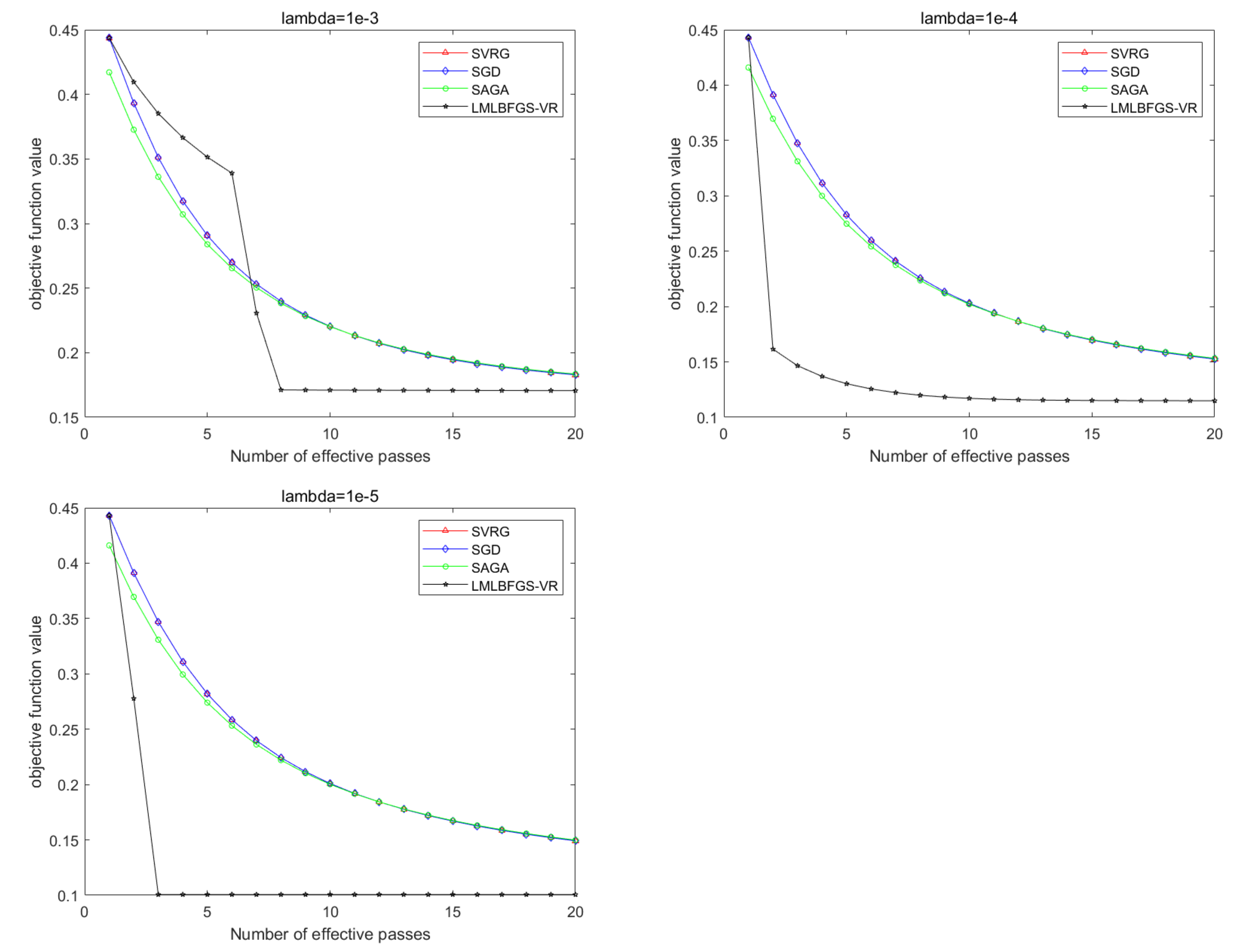
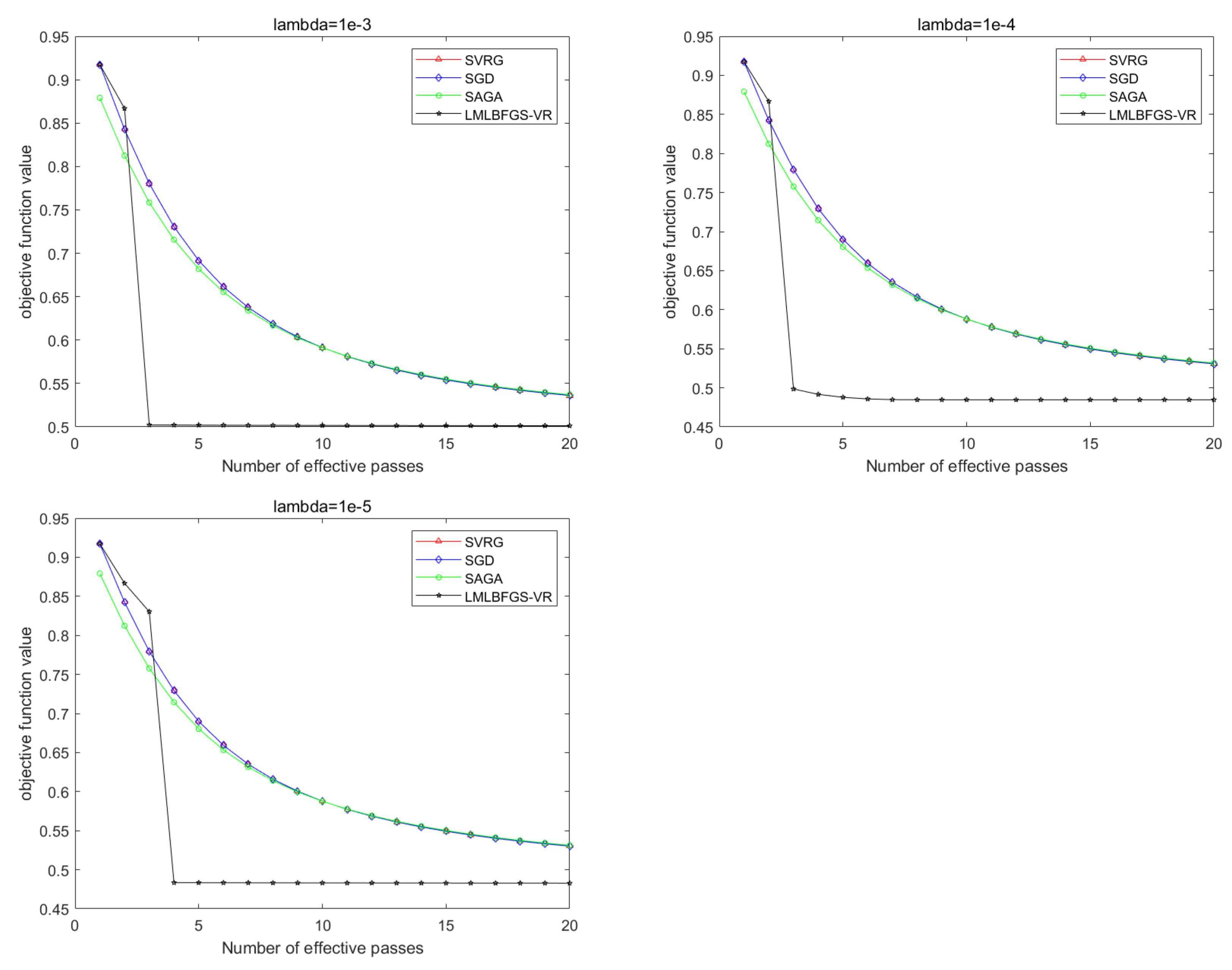
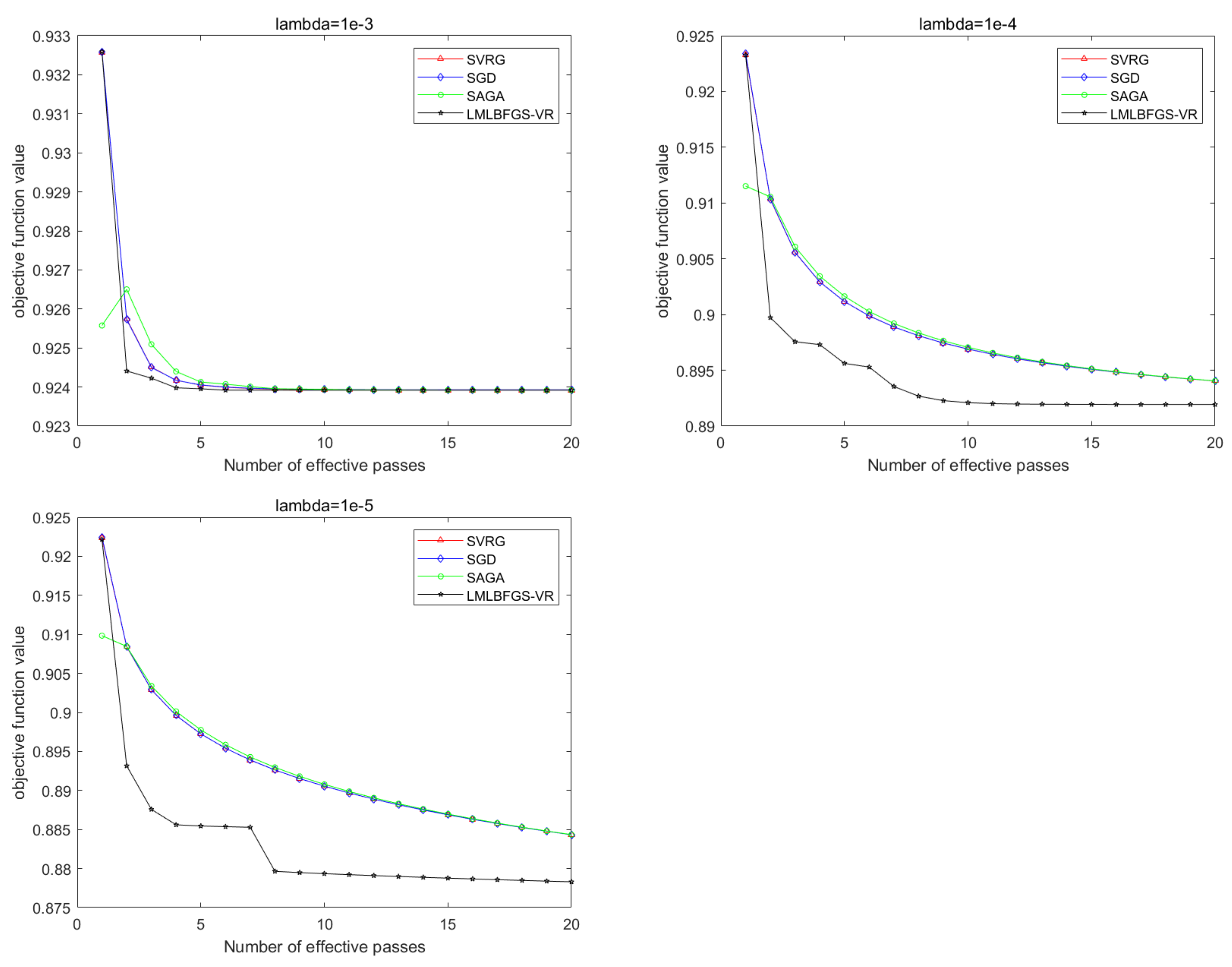
5. Numerical Results

In this section, we focus on the numerical performances of the proposed Algorithm 3 for solving nonconvex empirical risk minimization (ERM) problems and nonconvex support vector machine (SVM) problems.

5.1. Experiments with Synthetic Datasets

The models of the nonconvex SVM problems and nonconvex ERM problems are given as follows: $\lambda >0$ is a regularization parameter.

Problem 1.

The ERM problem with a nonconvex sigmoid loss function [13,14] is formulated as follows:

$$\underset{x\in {\Re }^{D_x}}{min}\frac{1}{n}\sum _{i=1}^n{f}_i(x)+\frac{\lambda }{2}{\parallel x\parallel }_2^2,f_i(x)=\frac{1}{1+exp(b_i{a}_i^{T}x)},$$

(54)

where $a_i\in {\Re }^d$ and $b_i\in \left\{-1,1\right\}$ represent the feature vector and corresponding label, respectively.

Problem 2.

The nonconvex support vector machine (SVM) problem with a sigmoid loss function [15,16] is formulated as follows:

$$\underset{x\in {\Re }^{D_x}}{min}\frac{1}{n}\sum _{i=1}^n{f}_i(x)+\lambda {\parallel x\parallel }^2,f_i(x)=1-tanh(b_i⟨x,a_i⟩).$$

(55)

We compare the proposed LMLBFGS-VR algorithm with SGD [1], SVRG [17] and SAGA [18], where the LMLBFGS-VR algorithms use a descent step size and other algorithms use a constant step size ${\alpha }_k$. The data sets in our experiments including Adult, IJCNN, Mnist, and Coctype. All the codes are written in MATLAB 2018b on a PC with AMD Ryzen 7 5800H with Radeon Graphics 3.20 GHz and 16 GB of memory.

5.2. Numerical Results for Problem 1

In this subsection, we present the numerical results of LMLBFGS-VR, SGD, SVRG, and SAGA for solving Problem 1 on the four data sets. For LMLBFGS-VR algorithms, the step size is ${\alpha }_k=0.02\times k^{-0.6}$, and the memory size is $r=10$ and $m=1\times {10}^{-5}$. The step size of other algorithms is chosen as 0.02. The number of inner loop q we chose as $n/V$ uniformly, where V is the batch size. The batch-size is set to 100 for Adult, IJCNN, and Covtype, and for Mnist. In order to further test the performance of the algorithm, the regularization parameter is set to ${10}^{-3},{10}^{-4}$, or ${10}^{-5}$. The following pictures demonstrate the performance of different algorithms. Figure 1, Figure 2, Figure 3 and Figure 4 show the convergence performance of all the stochastic algorithms for solving Problem 1 with $\lambda =1\times {10}^{-3},\lambda =1\times {10}^{-4}$ or $\lambda =1\times {10}^{-5}$ on four different data sets. From Figure 1, Figure 2, Figure 3 and Figure 4, we obtain that all the algorithms can solve the problem successfully. However, the proposed LMLBFGS- VR algorithms have significantly faster convergence speed than other algorithms. It is clear that the proposed algorithms, especially LMLBFGS-VR, have a great advantage for solving nonconvex support vector machine problems.

Figure 1. Comparison of all the algorithms for solving Problem 1 on Adult. From left to right: $\lambda =1\times {10}^{-3},\lambda =1\times {10}^{-4},\lambda =1\times {10}^{-5}$.

Figure 2. Comparison of all the algorithms for solving Problem 1 on Covtype. From left to right: $\lambda =1\times {10}^{-3},\lambda =1\times {10}^{-4},\lambda =1\times {10}^{-5}$.

Figure 3. Comparison of all the algorithms for solving Problem 1 on IJCNN. From left to right: $\lambda =1\times {10}^{-3},\lambda =1\times {10}^{-4},\lambda =1\times {10}^{-5}$.

Figure 4. Comparison of all the algorithms for solving Problem 1 on mnist. From left to right: $\lambda =1\times {10}^{-3},\lambda =1\times {10}^{-4},\lambda =1\times {10}^{-5}$.

5.3. Numerical Results for Problem 2

The numerical results of LMLBFGS-VR, SGD, SVRG, and SAGA for solving Problem 2 on the four data sets are presented in this subsection. All parameters are the same as the above subsection, and the regularization parameter is also set to $1\times {10}^{-3},1\times {10}^{-4},$ or $1\times {10}^{-5}$. The following figures demonstrate the performance of all the stochastic algorithms. The y-axis is the objective function value, and the x-axis denotes the number of effective passes, where computing a full gradient or evaluatingncomponent gradients is regarded as an effective pass. Figure 4, Figure 5, Figure 6, Figure 7 and Figure 8 demonstrate that the convergence performance of our LMLBFGS-VR algorithms on the four data sets, which show that they remarkably outperform the other algorithms. When $\lambda =1\times {10}^{-3}$, the objective function is almost minimized by two effective passes. In contrast, the SGD, SVRG, and SAGA algorithms converge slightly slowly, where these algorithms only use first-order information. Due to the use of second-order information and limited memory technique, LMLBFGS-VR requires only a few effective passes to quickly minimize the function value. From Figure 4, Figure 5, Figure 6, Figure 7 and Figure 8, we find that, as $\lambda$ decreases, the value of the function decreases to a smaller value. Thus, we can choose a smaller $\lambda$ for practical problems. Combined with the previous discussion, our LMLBFGS-VR algorithms make great progress in improving the computing efficiency for nonconvex machine learning problems.

Figure 5. Comparison of all the algorithms for solving Problem 2 on Adult. From left to right: $\lambda =1\times {10}^{-3},\lambda =1\times {10}^{-4},\lambda =1\times {10}^{-5}$.

Figure 6. Comparison of all the algorithms for solving Problem 2 on Covtype. From left to right: $\lambda =1\times {10}^{-3},\lambda =1\times {10}^{-4},\lambda =1\times {10}^{-5}$.

Figure 7. Comparison of all the algorithms for solving Problem 2 on IJCNN. From left to right: $\lambda =1\times {10}^{-3},\lambda =1\times {10}^{-4},\lambda =1\times {10}^{-5}$.

Figure 8. Comparison of all the algorithms for solving Problem 2 on mnist. From left to right: $\lambda =1\times {10}^{-3},\lambda =1\times {10}^{-4},\lambda =1\times {10}^{-5}$.

6. Conclusions

In this paper, we proposed one efficient modified stochastic limited BFGS algorithms for solving nonconvex stochastic optimization. The proposed algorithms can preserve the positive definiteness of $Hk$ without any convexity properties. The LMLBFGS-VR method with variance reduction was also presented to solve nonconvex stochastic optimization problems. Numerical experiments on nonconvex SVM problems and nonconvex ERM problems were performed to demonstrate the performance of the proposed algorithms, and the results indicated that our algorithms are comparable to other similar methods. In the future, we could consider the following points: (i) Whether we can use a proper line search to determine an appropriate step size, which can reduce the complexity and enhance the accuracy of the algorithm. (ii) Further experiments on the practical problems could be performed in the future to check the performance of the presented algorithms.

References

- Robbins, H.; Monro, S. A stochastic approximation method. Ann. Math. Stat. 1951, 22, 400–407. [Google Scholar] [CrossRef]
- Chung, K.L. On a stochastic approximation method. Ann. Math. Stat. 1954, 25, 463–483. [Google Scholar] [CrossRef]
- Polyak, B.T.; Juditsky, A.B. Acceleration of stochastic approximation by averaging. SIAM J. Control Optim. 1992, 30, 838–855. [Google Scholar] [CrossRef]
- Ruszczyǹski, A.; Syski, W. A method of aggregate stochastic subgradients with online stepsize rules for convex stochastic programming problems. In Stochastic Programming 84 Part II; Springer: Berlin/Heidelberg, Germany, 1986; pp. 113–131. [Google Scholar]
- Wright, S.; Nocedal, J. Numerical Optimization; Springer: Berlin/Heidelberg, Germany, 1999; Volume 35, p. 7. [Google Scholar]
- Bordes, A.; Bottou, L. SGD-QN: Careful quasi-Newton stochastic gradient descent. J. Mach. Learn. Res. 2009, 10, 1737–1754. [Google Scholar]
- Byrd, R.H.; Hansen, S.L.; Nocedal, J.; Singer, Y. A stochastic quasi-Newton method for large-scale optimization. SIAM J. Optim. 2016, 26, 1008–1031. [Google Scholar] [CrossRef]
- Gower, R.; Goldfarb, D.; Richtárik, P. Stochastic block BFGS: Squeezing more curvature out of data. In Proceedings of the 33rd International Conference on Machine Learning, New York, NY, USA, 19–24 June 2016; Volume 48, pp. 1869–1878. [Google Scholar]
- Covei, D.P.; Pirvu, T.A. A stochastic control problem with regime switching. Carpathian J. Math. 2021, 37, 427–440. [Google Scholar] [CrossRef]
- Wei, Z.; Li, G.; Qi, L. New quasi-Newton methods for unconstrained optimization problems. Appl. Math. Comput. 2006, 175, 1156–1188. [Google Scholar] [CrossRef]
- Durrett, R. Probability: Theory and Examples; Cambridge University Press: Cambridge, UK, 2019. [Google Scholar]
- Deng, N.Y.; Li, Z.F. Ome global convergence properties of a conic-variable metric algorithm for minimization with inexact line searches. Numer. Algebra Control Optim. 1995, 5, 105–122. [Google Scholar]
- Allen-Zhu, Z.; Hazan, E. Variance reduction for faster non-convex optimization. In Proceedings of the 33rd International Conference on Machine Learning, New York, NY, USA, 19–24 June 2016; Volume 48, pp. 699–707. [Google Scholar]
- Shalev-Shwartz, S.; Shamir, O.; Sridharan, K. Learning kernel-based halfspaces with the 0–1 loss. SIAM J. Comput. 2011, 40, 1623–1646. [Google Scholar] [CrossRef] [Green Version]
- Ghadimi, S.; Lan, G. Stochastic first-and zeroth-order methods for nonconvex stochastic programming. SIAM J. Optim. 2013, 23, 2341–2368. [Google Scholar] [CrossRef] [Green Version]
- Mason, L.; Baxter, J.; Bartlett, P.; Frean, M. Boosting algorithms as gradient descent in function space. Proc. Adv. Neural Inf. Process. Syst. 1999, 12, 512–518. [Google Scholar]
- Johnson, R.; Zhang, T. Accelerating stochastic gradient descent using predictive variance reduction. Adv. Neural Inf. Process. Syst. 2013, 26, 315–323. [Google Scholar]
- Defazio, A.; Bach, F.; Lacoste-Julien, S. SAGA: A fast incremental gradient method with support for non-strongly convex composite objectives. In Proceedings of the Advances in Neural Information Processing Systems, Montreal, QC, Canada, 8–13 December 2014; pp. 1646–1654. [Google Scholar]
Publisher’s Note: MDPI stays neutral with regard to jurisdictional claims in published maps and institutional affiliations. |
© 2022 by the authors. Licensee MDPI, Basel, Switzerland. This article is an open access article distributed under the terms and conditions of the Creative Commons Attribution (CC BY) license (https://creativecommons.org/licenses/by/4.0/).