
Adaptive Memory-Controlled Self-Attention for Polyphonic Sound Event Detection


Abstract
:1. Introduction
- A supervised memory-controlled attention model that improves sound event detection by a large margin, without manually optimizing towards dataset-specific attention width;
- Using the SOTA evaluation criterion, we verified our approach with two publicly available datasets;
- We studied the weakly-supervised SED pooling strategy on DCASE 2021 task4. This result can be a reference for pooling selection.
2. Related Work
2.1. Basic Systems Structures
2.2. Weakly-Supervised Sound Event Detection
3. Methods
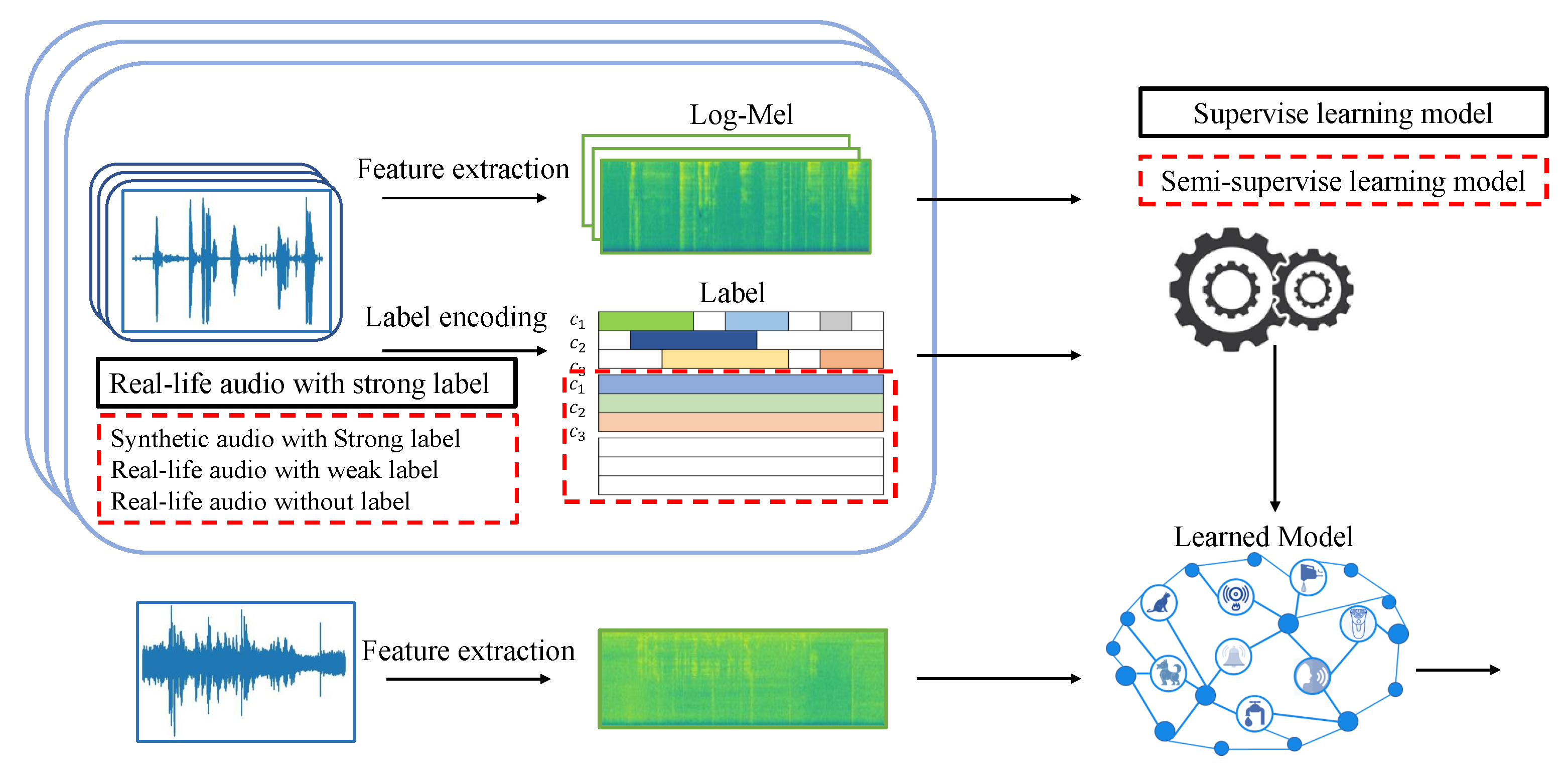
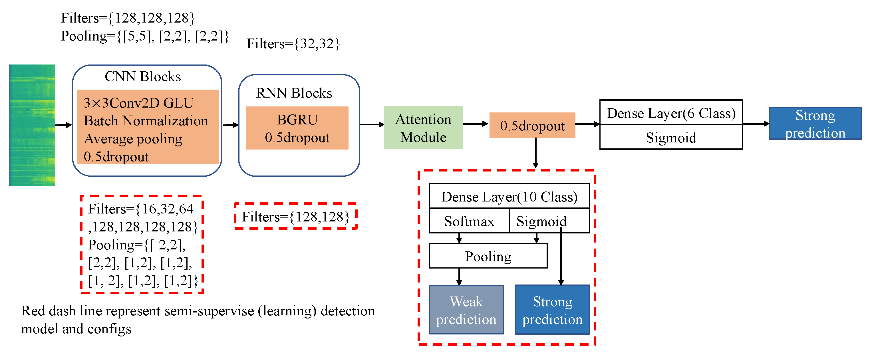
3.1. Model Overview
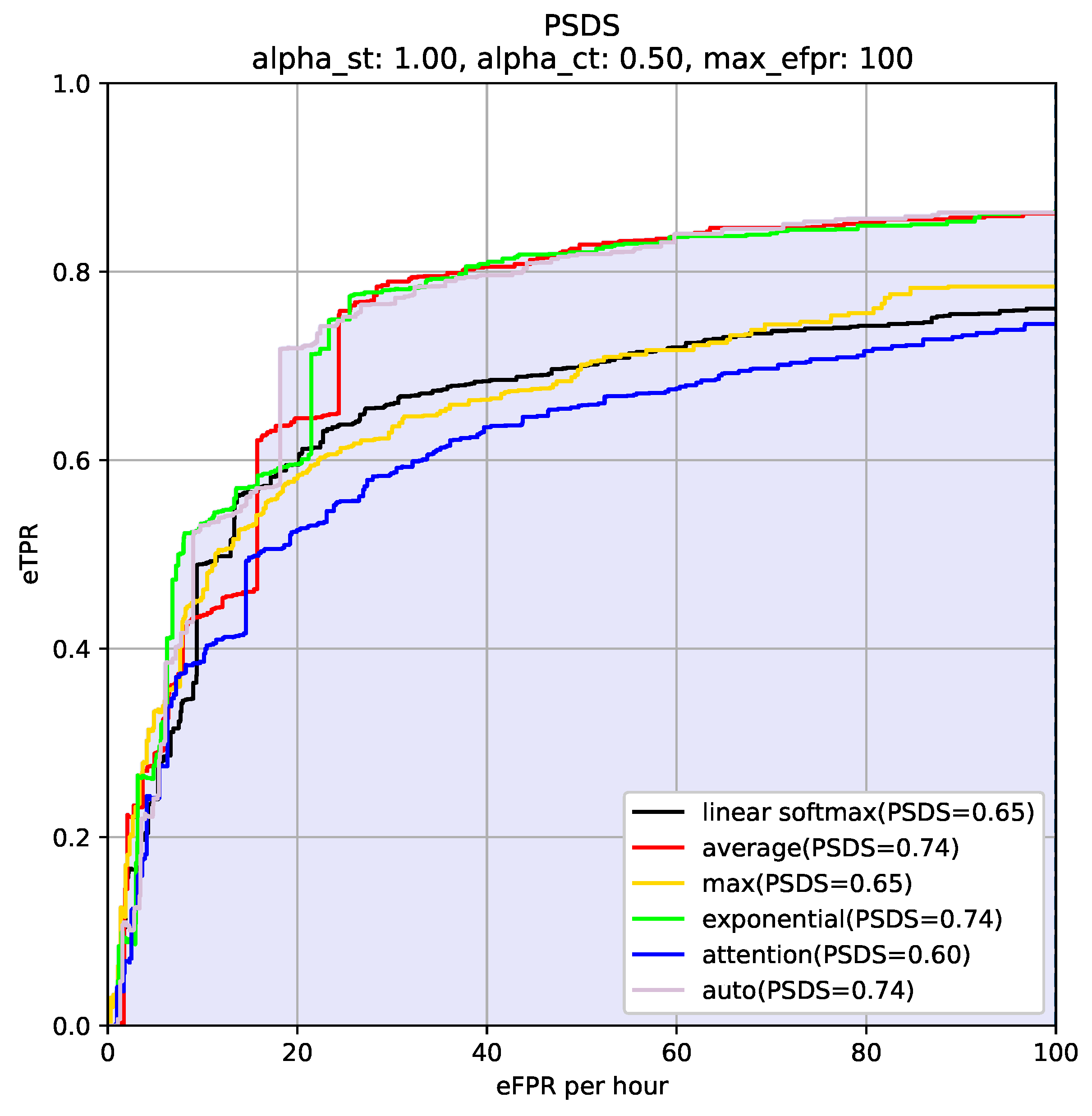
3.2. Pooling Function
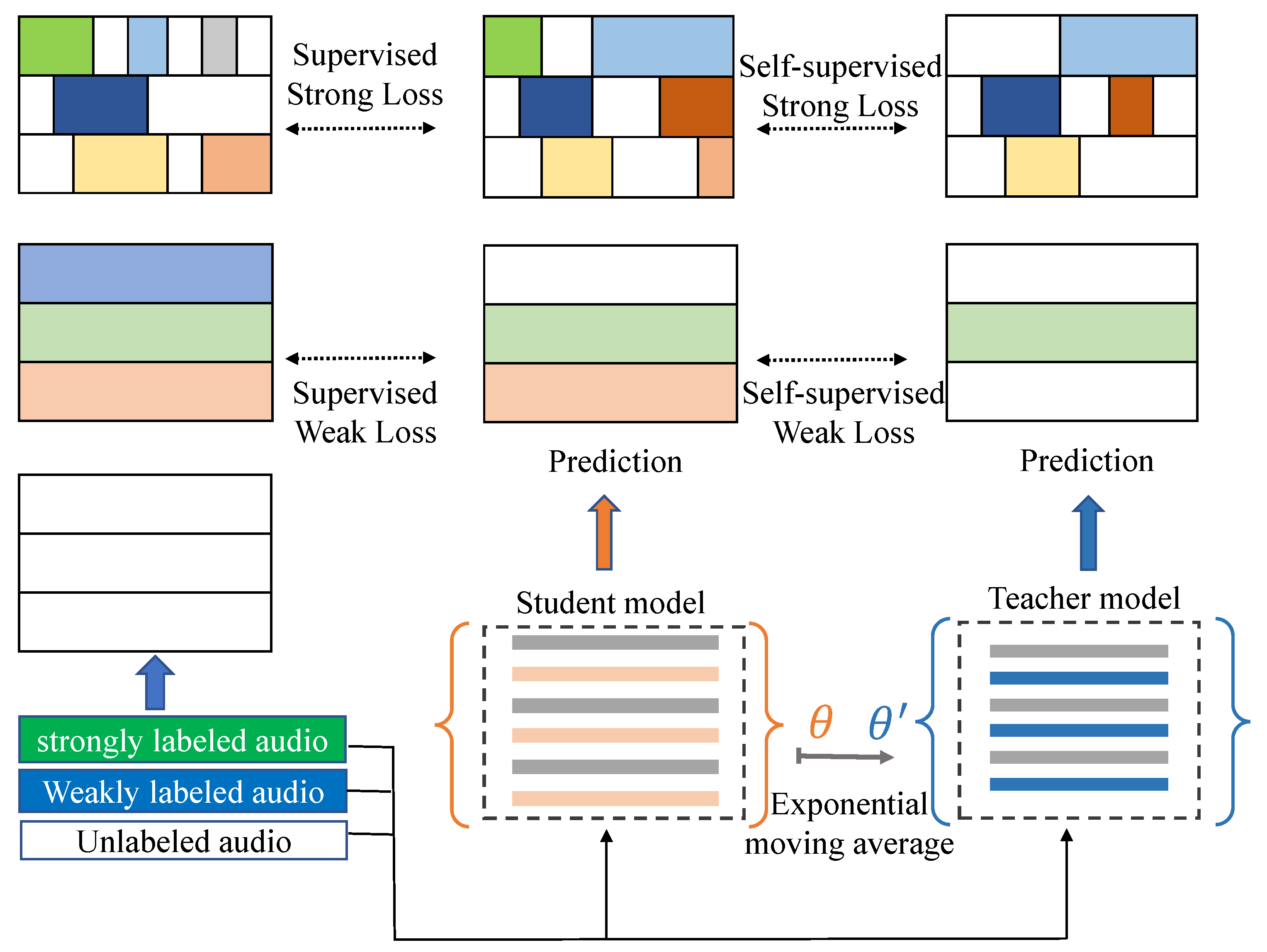
3.3. Semi-Supervised Model
3.4. Self-Attention Mechanism
3.5. Adaptive Memory-Controlled Self-Attention
4. Experiment
4.1. DCASE 2017 Task3
4.2. DCASE 2021 Task4
4.3. Evaluation Criterion
- (1)
- Polyphonic SED metrics. There are two ways of comparing system outputs and ground truth with polyphonic SED metrics: segment-based and event-based. Segment-based metrics compare system outputs and ground truth in short time segments, e.g., 1 s. Event-based metrics compare system outputs and ground truth event by event. Tolerance is allowed, e.g., a ms collar. In this paper, we use segment-based F-score, event-based F-score, and segment-wise error rate. F-score F is calculated as follows:Note that the segment-based and event-based Precision P, Recall R, and F-score F are calculated based on corresponding intermediate statistics. TP is the number of True Positive, FP is the number of false positives, and FN is the number of false negatives. The error rate measures the amount of errors in terms of insertions (I), deletions (D), substitutions (S) and the number of active sound event N in segment k.:
- (2)
- PSDS metrics. PSDS metrics allow for system comparisons independently from operating points (OPs) and provide more global insights into system performance. Furthermore, by specifying a system’s parameters, it can be tuned to varying applications in order to match a variety of user experience requirements. As in [27], we used predefined detection tolerance criterion (DTC) , ground truth tolerance criterion (GTC) , and the cross-trigger tolerance criterion (CTTC) . We then computed the TP ratio , FP ratio , the CR rate , then we have the effective FP rate (eFPR):In Equation (25), is a weighting parameter, is the sound event class, and is the total number of classes.Using both the exception (Equation (26)) and standard deviation (Equation (27)) of TP ratios across classes, the effective TP ratio (eTPR) is computed as eTPR: , where adjusts the cost of instability across classes. The coordinates of form the PSD ROC curve. The normalized area under the PSD curve is the PSD score (PSDS). Given dataset ground truth Y, and the set of evaluation parameters, , a PSDS of a system detection is:where is the maximum eFPR value of interest for the SED application under evaluation.In DCASE 2021 task4, the system detection will be evaluated in two scenarios that emphasize different system properties as follows. In scenario 1, the system needs to react fast upon event detection (e.g., to trigger an alarm or adapt a home automation system). The localization of the sound event is then very important. The PSDS parameters reflecting these needs are:
- -
- Detection tolerance criterion : 0.7;
- -
- Ground truth intersection criterion : 0.7;
- -
- Cross-trigger tolerance criterion : 0.3;
- -
- Cost of CTs on user experience : 0;
- -
- Cost of instability across class : 1.
In scenario 2, the system must avoid confusing between classes, but the reaction time is less crucial than in the first scenario. The PSDS parameters reflecting these needs are:- -
- Detection tolerance criterion : 0.1;
- -
- Ground truth intersection. Criterion : 0.1;
- -
- Cross-trigger tolerance criterion : 0.3;
- -
- Cost of CTs on user experience : 0.5;
- -
- Cost of instability across class : 1.
4.4. Implementation Details
5. Discussion
Experimental Results and Analysis
6. Conclusions
Author Contributions
Funding
Institutional Review Board Statement
Informed Consent Statement
Data Availability Statement
Conflicts of Interest
References
- Mesaros, A.; Diment, A.; Elizalde, B.; Heittola, T.; Vincent, E.; Raj, B.; Virtanen, T. Sound event detection in the DCASE 2017 challenge. IEEE/ACM Trans. Audio Speech Lang. Process. 2019, 27, 992–1006. [Google Scholar] [CrossRef] [Green Version]
- Serizel, R.; Turpault, N.; Eghbal-Zadeh, H.; Shah, A.P. Large-scale weakly labeled semi-supervised sound event detection in domestic environments. In Proceedings of the Detection and Classification of Acoustic Scenes and Events 2018 Workshop (DCASE2018), Surrey, UK, 19–23 November 2018; Available online: https://hal.inria.fr/hal-01850270 (accessed on 1 November 2018).
- Turpault, N.; Serizel, R.; Salamon, J.; Shah, A.P. Sound event detection in domestic environments with weakly labeled data and soundscape synthesis. In Proceedings of the Workshop on Detection and Classification of Acoustic Scenes and Events, New York, NY, USA, 25–26 October 2019; Available online: https://hal.inria.fr/hal-02160855 (accessed on 16 July 2019).
- Foggia, P.; Petkov, N.; Saggese, A.; Strisciuglio, N.; Vento, M. Reliable detection of audio events in highly noisy environments. Pattern Recognit. Lett. 2015, 65, 22–28. [Google Scholar] [CrossRef]
- Crocco, M.; Cristani, M.; Trucco, A.; Murino, V. Audio surveillance: A systematic review. ACM Comput. Surv. (CSUR) 2016, 48, 1–46. [Google Scholar] [CrossRef]
- Koutini, K.; Eghbal-zadeh, H.; Dorfer, M.; Widmer, G. The Receptive Field as a Regularizer in Deep Convolutional Neural Networks for Acoustic Scene Classification. In Proceedings of the 2019 27th European Signal Processing Conference (EUSIPCO), La Coruña, Spain, 2–6 September 2019; pp. 1–5. [Google Scholar] [CrossRef] [Green Version]
- Adavanne, S.; Politis, A.; Virtanen, T. Multichannel Sound Event Detection Using 3D Convolutional Neural Networks for Learning Inter-channel Features. In Proceedings of the 2018 International Joint Conference on Neural Networks (IJCNN), Rio de Janeiro, Brazil, 8–13 July 2018; pp. 1–7. [Google Scholar] [CrossRef] [Green Version]
- Virtanen, T.; Plumbley, M.D.; Ellis, D. Computational Analysis of Sound Scenes and Events; Springer: Berlin/Heidelberg, Germany, 2018; Chapter 2; pp. 13–25. [Google Scholar]
- Cao, Y.; Kong, Q.; Iqbal, T.; An, F.; Wang, W.; Plumbley, M.D. Polyphonic sound event detection and localization using a two-stage strategy. arXiv 2019, arXiv:1905.00268. [Google Scholar]
- Adavanne, S.; Pertilä, P.; Virtanen, T. Sound Event Detection Using Spatial Features and Convolutional Recurrent Neural Network. In Proceedings of the 2017 IEEE International Conference on Acoustics, Speech and Signal Processing (ICASSP) IEEE, New Orleans, LA, USA, 5–9 March 2017. [Google Scholar]
- Vaswani, A.; Shazeer, N.; Parmar, N.; Uszkoreit, J.; Jones, L.; Gomez, A.N.; Kaiser, Ł.; Polosukhin, I. Attention is all you need. In Proceedings of the Advances in Neural Information Processing Systems (NIPS), Long Beach, CA, USA, 4–9 December 2017; pp. 5998–6008. [Google Scholar]
- Li, N.; Liu, S.; Liu, Y.; Zhao, S.; Liu, M.; Zhou, M. Close to human quality TTS with Transformer. arXiv 2018, arXiv:1809.08895. [Google Scholar]
- Dong, L.; Shuang, X.; Bo, X. Speech-Transformer: A No-Recurrence Sequence-to-Sequence Model for Speech Recognition. In Proceedings of the ICASSP 2018—2018 IEEE Interna-tional Conference on Acoustics, Speech and Signal Pro-cessing (ICASSP), Calgary, AB, Canada, 15–20 April 2018. [Google Scholar]
- Wang, Y.; Metze, F. A first attempt at polyphonic sound event detection using connectionist temporal classification. In Proceedings of the 2017 IEEE International Conference on Acoustics, Speech and Signal Processing (ICASSP), New Orleans, LA, USA, 5–9 March 2017; pp. 2986–2990. [Google Scholar]
- Chen, Y.; Jin, H. Rare Sound Event Detection Using Deep Learning and Data Augmentation. In Proceedings of the Interspeech, Graz, Austria, 15–19 September 2019; pp. 619–623. [Google Scholar] [CrossRef]
- Kim, B.; Ghaffarzadegan, S. Self-supervised Attention Model for Weakly Labeled Audio Event Classification. In Proceedings of the 2019 27th European Signal Processing Conference (EUSIPCO), La Coruna, Spain, 2–6 September 2019. [Google Scholar]
- Kong, Q.; Yong, X.; Wang, W.; Plumbley, M.D. Audio Set Classification with Attention Model: A Probabilistic Perspective. In Proceedings of the International Conference on Acoustics, Speech, and Signal Processing, ICASSP 2018, Seoul, Korea, 15–20 April 2018. [Google Scholar]
- Wang, J.; Li, S. Self-attention mechanism based system for DCASE2018 challenge Task1 and Task4. In Proceedings of the DCASE Challenge, Surrey, UK, 19–20 November 2018; pp. 1–5. [Google Scholar]
- Sukhbaatar, S.; Grave, E.; Bojanowski, P.; Joulin, A. Adaptive Attention Span in Transformers. In Proceedings of the 57th Annual Meeting of the Association for Computational Linguistics, Florence, Italy, 28 July–2 August 2019. [Google Scholar]
- Dai, Z.; Yang, Z.; Yang, Y.; Carbonell, J.; Le, Q.V.; Salakhutdinov, R. Transformer-XL: Attentive Language Models beyond a Fixed-Length Context. In Proceedings of the 57th Annual Meeting of the Association for Computational Linguistics, Florence, Italy, 28 July–2 August 2019. [Google Scholar]
- Pankajakshan, A.; Bear, H.L.; Subramanian, V.; Benetos, E. Memory Controlled Sequential Self Attention for Sound Recognition. arXiv 2020, arXiv:2005.06650. [Google Scholar]
- Kim, B.; Pardo, B. Sound Event Detection Using Point-Labeled Data. In Proceedings of the 2019 IEEE Workshop on Applications of Signal Processing to Audio and Acoustics (WASPAA), New Paltz, NY, USA, 20–23 October 2019. [Google Scholar]
- Kim, B.; Pardo, B. A human-in-the-loop system for sound event detection and annotation. ACM Trans. Interact. Intell. Syst. Tiis 2018, 8, 13. [Google Scholar] [CrossRef]
- Kumar, A.; Raj, B. Audio event detection using weakly labeled data. In Proceedings of the 24th ACM International Conference on Multimedia, Amsterdam, The Netherlands, 15–19 October 2016; pp. 1038–1047. [Google Scholar]
- Frederic, F.; Annamaria, M.; Daniel, E.; Eduardo, F.; Magdalena, F.; Benjamin, E. Proceedings of the 6th Workshop on Detection and Classification of Acoustic Scenes and Events (DCASE 2021), Online. 15–19 November 2021.
- Tarvainen, A.; Valpola, H. Mean teachers are better role models: Weight-averaged consistency targets improve semi-supervised deep learning results. arXiv 2017, arXiv:1703.01780. [Google Scholar]
- Bilen, Ç.; Ferroni, G.; Tuveri, F.; Azcarreta, J.; Krstulović, S. A Framework for the Robust Evaluation of Sound Event Detection. In Proceedings of the ICASSP 2020—2020 IEEE International Conference on Acoustics, Speech and Signal Processing (ICASSP), Barcelona, Spain, 4–8 May 2020; pp. 61–65. [Google Scholar] [CrossRef] [Green Version]
- McFee, B.; Salamon, J.; Bello, J.P. Adaptive Pooling Operators for Weakly Labeled Sound Event Detection. IEEE/ACM Trans. Audio Speech Lang. Process. 2018, 26, 2180–2193. [Google Scholar] [CrossRef] [Green Version]
- Wang, Y.; Li, J.; Metze, F. A Comparison of Five Multiple Instance Learning Pooling Functions for Sound Event Detection with Weak Labeling. In Proceedings of the ICASSP 2019—2019 IEEE International Conference on Acoustics, Speech and Signal Processing (ICASSP), Brighton, UK, 2–17 May 2019; pp. 31–35. [Google Scholar] [CrossRef] [Green Version]
- Lin, L.; Wang, X.; Liu, H.; Qian, Y. Specialized Decision Surface and Disentangled Feature for Weakly-Supervised Polyphonic Sound Event Detection. IEEE/ACM Trans. Audio Speech Lang. Process. 2020, 28, 1466–1478. [Google Scholar] [CrossRef] [Green Version]
- Kong, Q.; Yu, C.; Xu, Y.; Iqbal, T.; Wang, W.; Plumbley, M.D. Weakly Labelled AudioSet Tagging With Attention Neural Networks. IEEE/ACM Trans. Audio Speech Lang. Process. 2019, 27, 1791–1802. [Google Scholar] [CrossRef] [Green Version]
- Dinkel, H.; Wu, M.; Yu, K. Towards Duration Robust Weakly Supervised Sound Event Detection. IEEE/ACM Trans. Audio Speech Lang. Process. 2021, 29, 887–900. [Google Scholar] [CrossRef]
- Su, T.-W.; Liu, J.-Y.; Yang, Y.-H. Weakly-supervised audio event detection using event-specific gaussian filters and fully convolutional networks. In Proceedings of the 2017 IEEE International Conference on Acoustics, Speech and Signal Processing (ICASSP), New Orleans, LA, USA, 5–9 March 2017; pp. 791–795. [Google Scholar]
- Kumar, A.; Khadkevich, M.; Fugen, C. Knowledge transfer from weakly labeled audio using convolutional neural network for sound events and scenes. In Proceedings of the 2018 IEEE International Conference on Acoustics, Speech and Signal Processing (ICASSP), Calgary, AB, Canada, 15–20 April 2018; pp. 326–330. [Google Scholar]
- Xu, Y.; Kong, Q.; Wang, W.; Plumbley, M.D. Large-scale weakly supervised audio classification using gated convolutional neural network. In Proceedings of the 2018 IEEE International Conference on Acoustics, Speech and Signal Processing (ICASSP), Calgary, AB, Canada, 15–20 April 2018; pp. 121–125. [Google Scholar]
- Chung, J.; Gulcehre, C.; Cho, K.; Bengio, Y. Empirical Evaluation of Gated Recurrent Neural Networks on Sequence Modeling. arXiv 2014, arXiv:1412.3555. [Google Scholar]
- Bahdanau, D.; Cho, K.; Bengio, Y. Neural machine translation by jointly learning to align and translate. In Proceedings of the International Conference on Learning Representations (ICLR), Banff, AB, Canada, 14–16 April 2014. [Google Scholar]
- Mesaros, A.; Heittola, T.; Virtanen, T. Metrics for polyphonic sound event detection. Appl. Sci. 2016, 6, 162. [Google Scholar] [CrossRef]
- Zhang, H.; Cisse, M.; Dauphin, Y.N.; Lopez-Paz, D. mixup: Beyond empirical risk minimization. In Proceedings of the International Conference on Learning Representations, Vancouver, BC, Canada, 30 April–3 May 2018. [Google Scholar]
- Nam, H.; Kim, S.H.; Park, Y.H. FilterAugment: An Acoustic Environmental Data Augmentation Method. arXiv 2021, arXiv:2110.03282. [Google Scholar]
- Adavanne, S.; Virtanen, T. A report on sound event detection with different binaural features. arXiv 2017, arXiv:1710.02997. [Google Scholar]
- Mesaros, A.; Heittola, T.; Diment, A.; Elizalde, B.; Shah, A.; Vincent, E.; Raj, B.; Virtanen, T. DCASE 2017 challenge setup: Tasks, datasets and baseline system. In Proceedings of the Detection and Classification of Acoustic Scenes and Events 2017 Workshop (DCASE2017), Munich, Germany, 16–17 November 2017; pp. 85–92. [Google Scholar]
- Zheng, X.; Song, Y.; McLoughlin, I.; Liu, L.; Dai, L.-R. An Improved Mean Teacher Based Method for Large Scale Weakly Labeled Semi-Supervised Sound Event Detection. In Proceedings of the ICASSP 2021—2021 IEEE International Conference on Acoustics, Speech and Signal Processing (ICASSP), Toronto, ON, Canada, 6–11 June 2021; pp. 356–360. [Google Scholar] [CrossRef]
- Wang, Y.W.; Chen, C.P.; Lu, C.L.; Chan, B.C. Semi-Supervised Sound Event Detection Using Multiscale Channel Attention and Multiple Consistency Training. In Proceedings of the 6th Workshop on Detection and Classification of Acoustic Scenes and Events (DCASE 2021), Online. 15–19 November 2021. [Google Scholar]
- Dinkel, H.; Cai, X.; Yan, Z.; Wang, Y.; Zhang, J.; Wang, Y. A lightweight approach for semi-supervised sound event detection with unsupervised data augmentation. In Proceedings of the 6th Workshop on Detection and Classification of Acoustic Scenes and Events (DCASE 2021), Online. 15–19 November 2021. [Google Scholar]
- Kong, Q.; Xu, Y.; Wang, W.; Plumbley, M.D. A joint detection-classification model for audio tagging of weakly labelled data. In Proceedings of the 2017 IEEE International Conference on Acoustics, Speech and Signal Processing (ICASSP), New Orleans, LA, USA, 5–9 March 2017; pp. 641–645. [Google Scholar] [CrossRef] [Green Version]
- Hershey, S.; Ellis, D.P.; Fonseca, E.; Jansen, A.; Liu, C.; Moore, R.C.; Plakal, M. The Benefit of Temporally-Strong Labels in Audio Event Classification. In Proceedings of the ICASSP 2021—2021 IEEE International Conference on Acoustics, Speech and Signal Processing (ICASSP), Toronto, ON, Canada, 6–11 June 2021. [Google Scholar]


| Detection System | Segment-Based | |
|---|---|---|
| Error Rate | F1-Score | |
| Baseline [42] | 0.9358 | 42.8% |
| Winner system [41] | 0.7914 | 41.7% |
| Attention width 20 | 0.711 | 48.3% |
| Attention width 50 | 0.7063 | 48.1% |
| Attention width 100 | 0.7065 | 47.4% |
| Attention width 200 | 0.6810 | 49.6% |
| Attention width 300 | 0.6980 | 49.5% |
| Adaptive strategy | 0.6927 | 49.6% |
| System | Event-Based | Segment-Based | |||||
|---|---|---|---|---|---|---|---|
| PSDS1 | PSDS2 | Total | F-Score | Error Rate | F-Score | Error Rate | |
| max pooling [33] | 0.37 | 0.65 | 1.02 | 42.35% | 1.08 | 73.89% | 0.46 |
| avg pooling [34] | 0.06 | 0.74 | 0.80 | 18.71 % | 1.28 | 67.32 % | 0.83 |
| lin pooling [35] | 0.38 | 0.65 | 1.03 | 48.37 % | 0.94 | 76.88 | 0.45 |
| exp pooling [29] | 0.07 | 0.74 | 0.81 | 19.77 % | 1.27 | 67.84 % | 0.81 |
| attn pooling [31,46] | 0.39 | 0.60 | 0.99 | 46.08 % | 1.04 | 75.44 % | 0.46 |
| auto pooling [28] | 0.08 | 0.74 | 0.82 | 20.48 % | 1.26 | 68.11 % | 0.79 |
| attn20 | 0.14 | 0.65 | 0.79 | 19.87% | 1.09 | 63.12% | 0.58 |
| attn50 | 0.18 | 0.65 | 0.83 | 23.06% | 1.06 | 65.29% | 0.55 |
| attn100 | 0.17 | 0.62 | 0.79 | 24.79% | 1.05 | 64.66% | 0.56 |
| attn200 | 0.05 | 0.73 | 0.74 | 19.51% | 1.24 | 66.70% | 0.85 |
| Baseline [3] | 0.34 | 0.52 | 0.86 | ||||
| CNN-transformer [44] | 0.37 | 0.72 | 1.09 | ||||
| winner [43] | 0.45 | 0.74 | 1.19 | ||||
| light weight [45] | 0.37 | 0.60 | 0.97 | ||||
| best | 0.39 | 0.74 | 1.13 | ||||
Publisher’s Note: MDPI stays neutral with regard to jurisdictional claims in published maps and institutional affiliations. |
© 2022 by the authors. Licensee MDPI, Basel, Switzerland. This article is an open access article distributed under the terms and conditions of the Creative Commons Attribution (CC BY) license (https://creativecommons.org/licenses/by/4.0/).
Share and Cite
Wang, M.; Yao, Y.; Qiu, H.; Song, X. Adaptive Memory-Controlled Self-Attention for Polyphonic Sound Event Detection. Symmetry 2022, 14, 366. https://doi.org/10.3390/sym14020366
Wang M, Yao Y, Qiu H, Song X. Adaptive Memory-Controlled Self-Attention for Polyphonic Sound Event Detection. Symmetry. 2022; 14(2):366. https://doi.org/10.3390/sym14020366
Chicago/Turabian StyleWang, Mei, Yu Yao, Hongbin Qiu, and Xiyu Song. 2022. "Adaptive Memory-Controlled Self-Attention for Polyphonic Sound Event Detection" Symmetry 14, no. 2: 366. https://doi.org/10.3390/sym14020366
APA StyleWang, M., Yao, Y., Qiu, H., & Song, X. (2022). Adaptive Memory-Controlled Self-Attention for Polyphonic Sound Event Detection. Symmetry, 14(2), 366. https://doi.org/10.3390/sym14020366