Abstract
In this paper, we propose a generalized explicit algorithm for approximating the common solution of generalized split feasibility problem and the fixed point of demigeneralized mapping in uniformly smooth and 2-uniformly convex real Banach spaces. The generalized split feasibility problem is a general mathematical problem in the sense that it unifies several mathematical models arising in (symmetry and non-symmetry) optimization theory and also finds many applications in applied science. We designed the algorithm in such a way that the convergence analysis does not need a prior estimate of the operator norm. More so, we establish the strong convergence of our algorithm and present some computational examples to illustrate the performance of the proposed method. In addition, we give an application of our result for solving the image restoration problem and compare with other algorithms in the literature. This result improves and generalizes many important related results in the contemporary literature.
Keywords:
demigeneralized mapping; fixed point; monotone mapping; mid-point method; strong convergence; Banach spaces MSC:
49J40; 58E35; 65K15; 90C33
1. Introduction
Let C and Q be nonempty, closed, and convex subsets of two real Hilbert spaces and , respectively, and be a bounded linear operator. The Split Feasibility Problem (shortly, SFP) is defined as
We denote the set of solutions of the SFP (1) by i.e., The SFP was first introduced by [1] in the setting of finite dimensional spaces, for modeling inverse problems arising from phrase retrievals and in medical image reconstruction. Since then, it has been studied widely and extended by many researchers mainly due to its applications in various areas such as radiation therapy treatment planning, signal processing, image restoration, computer tomography, etc., see e.g., [2,3,4,5].
In 2014, Ref. [6] introduced the Generalized Split Feasibility Problem (GSFP) in the framework of real Hilbert spaces as follows:
where is a maximal monotone operator, is a bounded linear operator, is a non-expansive mapping and is the set of fixed points of T, i.e., We denote the set of solution of the GSFP (2) by Note that, when (i.e., the normal cone operator at C) and , the GSFP reduces to the SFP. Ref. [6] proposed the following iterative method for solving the GSFP in real Hilbert spaces:
where is the resolvent operator of A and is the adjoint of They also proved that the sequence generated by (3) converges weakly to a solution of the GSFP. Recently, Ref. [7] extended the result of [6] to the setting of uniformly convex and 2-uniformly smooth real Banach spaces. They proposed the following iterative method in particular, for solving the GSFP in real Banach spaces:
where and are the normalized duality mapping on the real Banach spaces and , respectively, is a maximal monotone operator and and are nonexpansive mappings with The authors proved that the sequence generated by (4) converges weakly to an element in . Furthermore, Ref. [8] also introduced a strong convergence algorithm for finding a common element in the set of solution of GSFP and common fixed point problem for a countable family of nonexpansive mappings between a real Hilbert space H and real Banach space E as follows:
where is the metric projection from H onto C, is the normalized duality mapping on E, is a bounded linear operator, is a firmly nonexpansive-like mapping, is a countable family of demimetric mappings on C with , are sequences satisfying the following conditions:
- (i)
- and
- (ii)
- and
- (iii)
- (iv)
- and where
- (v)
- and
Very recently, Ref. [9] further introduced a Halpern-type strong convergence algorithm for solving the GSFP in real Banach spaces as follows:
where satisfying and is a -quasi-strictly pseudononspreading mappings such that The authors proved that the sequence generated by Algorithm (6) converges strongly to an element in under some mild conditions on the control sequences. Note that, in the methods mentioned above, the stepsize depends on prior estimates of the norm of the bounded linear operator, i.e., , which, in general, it is very difficult to estimate (see, e.g., [10]), thus the following question arises naturally:
Question A: Can we provide an iterative scheme which does not depend on a prior estimate of the norm of the bounded linear operator for solving the generalized split feasibility problem in real Banach spaces?
On the other hand, Ref. [11] introduced the generalized viscosity implicit rule for approximating the fixed point of a nonexpansive mapping in real Hilbert spaces as follows: given , compute
They also proved that the sequence generated by (7) converges strongly to a point in However, it was noted that the computation by implicit method is not a simple task in general. To overcome this difficulty, the explicit midpoint method was given by the following finite difference scheme which was originally introduced in the books [12,13]:
where is a contraction mapping and is the mesh. In 2017, Ref. [14] combined the generalized viscosity implicit midpoint method (7) with the explicit midpoint method (8) for approximating the fixed point problem of a quasi-nonexpansive mapping They introduced the following generalized viscosity explicit midpoint method in particular: for any and
They also showed that the sequence generated by (9) converges strongly to a fixed point of T under certain assumptions imposed on the parameters , and
Motivated by the above results, in this paper, we provide an affirmative answer to Question A using the technique above in real Banach spaces. In particular, we introduce a generalized explicit method for solving the GSFP without prior knowledge of the norm of the bounded operator in uniformly smooth and 2-uniformly convex real Banach spaces. The algorithm is designed such that its stepsize is determined self-adaptively at each iteration, and its convergence does not require prior estimate of the bounded linear operator norm. We also prove a strong convergence result for the sequence generated by the algorithm and also provide a numerical example to illustrate the performance of the iterative method. Furthermore, we utilize the algorithm to solves image restoration problem and also compare it performance with other related methods in the literature.
2. Preliminaries
In this section, we present some preliminary Definitions and concepts which are needed in this paper. Let E be a real Banach space with dual and denotes the unit sphere of E. We denote the value of at by . In addition, we denote the strong (resp. weak) convergence of a sequence to a point by (resp. ).
Let , be two Banach spaces and denotes the bounded linear operator. Then, the adjoint operator of B which is denoted by is defined as with for all and . is also bounded linear operator and
A Banach space E is said to be smooth if exists for each and for any , if for all with , then E is called strictly convex. In addition, E is said to be uniformly convex if, for any , there exists such that, if , then for all . The modulus of smoothness of E is the function defined by
In addition, E is called uniformly smooth if ; q-uniformly smooth if there exists a positive real number such that for any . Hence, every q-uniformly smooth Banach space is uniformly smooth. We know that and are q-uniformly smooth for ; 2-uniformly smooth and uniformly convex (see [15] for more details).
Furthermore, the normalized duality mapping is defined by
It is known that J has the following properties (for more details, see [16,17,18]):
- (UM1)
- If E is smooth, then J is single-valued.
- (UM2)
- If E is strictly convex, then J is one to one and strictly monotone.
- (UM3)
- If E is uniformly smooth, then J is uniformly norm to norm continuous on a bounded subset of E.
- (UM4)
- If E is smooth, strictly convex, and reflexive Banach space, then J is single-valued, one to one and onto.
- (UM5)
- If E is uniformly smooth and uniformly convex, then the dual space is also uniformly smooth and uniformly convex; furthermore, J and are both uniformly continuous on bounded subsets of E.
- (UM6)
- If E is a reflexive, strictly convex, and smooth Banach space, then (the duality mapping from into E) is single-valued, one to one and onto.
Let E be a Banach space and denotes the Lyapunov functional defined as
The functional satisfies the following properties (see [19]):
- (A1)
- (A2)
- (A3)
- ;
- (A4)
Remark 1.
If E is strictly convex, then, for all if and only if (See Remark 2.1 in [20]).
Now, we introduce another functional-like by [21], which is a mild modification and has a relationship with a Lyapunov functional as follows:
for all and . From the Definition of , we get
For each , the mapping g defined by for all is a continuous, convex function from into . The following Lemma is a very important property of V.
Lemma 1
([21]). Let E be a reflexive, strictly convex and smooth Banach space and let V be as in (10). Then,
for all and .
Let E a be reflexive, strictly convex and smooth Banach space and C a nonempty closed and convex subset of E. Then, by [21], for each , there exists a unique element (denoted by ) such that
The mapping , defined by , is called the generalized projection operator (see [22]), which has the following important characteristic.
Lemma 2
([23]). Let C be a nonempty, closed and convex subset of a smooth Banach space E, if . Then, if and only if
In the sequel, we shall use the following results.
Lemma 3
([19]). Let E be a uniformly smooth Banach space and . Then, there exists a continuous, strictly increasing and convex function such that and
for all and .
Lemma 4
([15]). Let E be a real uniformly convex Banach space and . Let Then, there exists a continuous strictly increasing convex function such that and
for all and .
Lemma 5
([20]). Let E be a uniformly convex and smooth Banach space and and be two sequences in E. If and either or is bounded, then
Lemma 6
([15]). Let E be a 2-uniformly convex and smooth real Banach space. Then, there exists a positive real-valued constant α such that
Lemma 7
([15]). Let E be a 2-uniformly smooth Banach space, then, for each and , the following holds:
Definition 1.
A mapping is said to be:
- (i)
- quasi-nonexpansive (see [20]) if and
- (ii)
- firmly nonexpansive type if for all , we have
- (iii)
- quasi-ϕ-strictly pseudocontractive (see [24]) if and there exists a constant such that
- (iv)
- -demigeneralized (see [25]) if and there exists and such that for any and , we haveIn particular, T is -demigeneralized mapping if and only if
A set-valued operator is said to be: (i) if for all , we have
where and (ii) maximal monotone if A is monotone and the graph of A i.e., is not properly contained in the graph of any other monotone operator. It is known that, when A is a maximal monotone operator and , then the resolvent of A is defined by for . More so, the null points of A is defined by . Note that is a closed and convex set, and , (see [18]).
Lemma 8
([26,27]). Let C be a nonempty, closed and convex subset of strictly convex, smooth and reflexive Banach space, and let and be a monotone operator such that . Then, the resolvent of A which is defined by for all is a firmly nonexpansive type mapping.
Lemma 9
([28]). Let E be a reflexive, smooth and strictly convex Banach space and a maximal monotone operator such that and for all . Then,
Lemma 10
([25]). Let E be a smooth Banach space and C be a nonempty closed and convex subset of E. Let η be a real number with and s be a real number with . Let U be an -demigeneralized mapping of C into E. Then, is closed and convex.
Lemma 11
([29]). Let E be a smooth Banach space and C a nonempty closed and convex subset of E. Let and be a -demigeneralized mapping with . Let λ be a real number in and define , where J is the duality mapping on E. Then, is a quasi-nonexpansive mapping of C into E and .
Lemma 12
([30]). If is a sequence of nonnegative real numbers satisfying the following inequality:
where and Then, as
Definition 2.
A self-mapping T on a Banach space is said to be demiclosed at y, if for any sequence which converges weakly to x, and if the sequence converges strongly to y, then . In particular, if , then T is demiclosed at 0.
Lemma 13
([31]). Let be a sequence of real numbers such that there exists a subsequence of such that for all . Then, there exists a nondecreasing sequence such that and the following properties are satisfied by all (sufficiently large) numbers :
In fact, .
3. Results
In this section, we present our algorithm and its convergence analysis as follows:
Theorem 1.
Let and be uniformly smooth and 2-uniformly convex real Banach spaces. Let be a -demigeneralized mapping and demiclosed at zero with and such that . Let be a -demigeneralized mapping and demiclosed at zero with such that . Let A be a maximal monotone operator of E into such that and are the generalized resolvent operator of A for . Let be a bijective bounded linear operator with its adjoint . Suppose that . Let be a sequence in such that and be a sequence generated by the following iterative scheme: given , compute
where and , , are sequences in and . Suppose the following conditions are satisfied:
- (C1)
- and ;
- (C2)
- for any as in Lemma 6 and any fixed value , the stepsize is chosen as follows:if ; otherwise, ().
- (C3)
- and , where .
Then, converges strongly to , where .
Remark 2.
Since and are and -demigeneralized mappings, respectively, then and are closed and convex sets by Lemma 10. Since is linear and bounded and exists, then is linear and bounded (continuous). Since is closed and convex, then is also closed and convex. is closed and convex (see [18] for details). Hence, is nonempty closed and convex. Therefore, from into Γ is well-defined.
Furthermore, since for any is relatively nonexpansive mapping and by Lemma 11. Let , we have that , , thus , and also . In addition, since is generalized resolvent for , then, from Lemma 8, we have that is firmly nonexpansive operator for , then for any , we have for all .
Proof.
Let , then, from Lemma 6, 7 and (15), we have
where the last estimation follows from the stepsize rule (18). In addition, from in (17) and (24), we have
and
Since converges, then it is bounded and so, with the help of (A1), there exists , such that . Now, letting , for all , in particular, . Assuming for some that , then, by (24), we have
Hence by induction, we obtain that for all . Therefore, is bounded.
Furthermore, from (19), (21) and (23), we get
From (C2), we have that hence
This implies that
Hence, from (25) and (26), we get
The remaining part of the proof will be divided into two cases.
Case I: Suppose that the sequence is non-increasing sequence of real numbers. Since this sequence is bounded, then it converges for all . That is,
Thus, from (C1), (C3), (27) and (28), we have
In addition, combining (C2), (C3) and (25), we have
It follows from (28) and (29) that
as . Since is uniformly smooth, then, from (UM5) and (30), we obtain
Furthermore, using (10) and Lemma 4, we get
In addition, with (20), (23) and (32), we get
Thus, from (C3) and (33), we obtain
Then, using (C1), we get
Using property of g in Lemma 4, we obtain
Since is uniformly smooth, then, from (34), we get
In addition, by Lemma 9, (20) and (23), we get
Thus, using (C3), we have
Then, applying (C1) and (28), we get
From Lemma 5, we get
Since is uniformly smooth, then
It follows from (35) and (36) that
Since is uniformly smooth, then is uniformly norm-to-norm continuous on bounded subsets if and from (38), we obtain
As we know that , thus
Since , it follows from (39) that
Thus, we have
In addition, since , then
It follows from (C1), (C3) and (28) that
Hence,
This implies that
In addition, from (A3) and (17), we get
It follows from (42) and (43) that
Thus, from Lemma 5, we get
Using Lemma 9, in (17) and by (22), we have
It follows from (C1) and (28) that
and, by Lemma 5, we have
Since
then it follows from (43), (45), (47) and (49) that
Furthermore, since is reflexive and is bounded, then there exists a subsequence of such that converges weakly to in . In addition, we know that B is linear and bounded, then it is continuous, so implies that . Thus, by (31), we have and, since U is demiclosed at zero, then, , that is, . From (30), we get , thus , so, using (36) it implies that converges weakly to . Since is generalized resolvent of A in , then
Since A is monotone, we have
for all and we know from (37) that , then, since for all , we have that for all and with the fact that A is maximal monotone, we obtain . In addition, since , we know from (41) that ; then, using the fact that T is demiclosed at zero, we obtain . Therefore, .
Next, we show that converges strongly to . Letting , since converges weakly to , then, using Lemma 2, we get
Observe that
It follows from (50) and (51) that
Finally, using (11), Lemma 1, and (22), we obtain
Thus, with the help of (C1), (52) and applying Lemma 12, we get as ; then, by Lemma 6, we obtain as . Hence, , where .
Case II: Suppose that is not a non-increasing sequence. Then, let be a subsequence of such that for all . Then, by Lemma 13, there exists a nondecreasing sequence such that as ,
Since is bounded, then exists. Therefore, using the same method of arguments as in Case I (from (30)–(50)), we get
Similarly as in the proof of Case 1, we obtain
In addition, from (53), we have
which implies
and, since for all and then
Hence, from (54), we obtain , then, with (55), we have . However, we know that for all , thus . Therefore, using Lemma 6, we obtain as . Hence, , where . This completes the proof. □
We obtained the following results as the consequences of our main result.
(i) Let C and Q be nonempty, closed, and a convex subset of and , respectively. Taking the normal cone operator at C which is maximally monotone (see [32]) and defined by
then the resolvent operator with respect to A is the projection operator . In addition, taking , the metric projection from onto Q, then the GSFP reduces to the SFP. Note that the class of (0,0)-demigeneralized mapping is nonexpansive. Hence, from Theorem 1, we obtained the following result for solving SFP in real Banach spaces.
Corollary 1.
Let C and Q be nonempty, closed and convex subsets of two uniformly smooth and 2-uniformly convex real Banach spaces and , respectively. Let and be normalized duality mappings on and , respectively. Let be a -demigeneralized mapping and demiclosed at zero with and such that . Let be a bijective bounded linear operator with its adjoint . Suppose that . Let be a sequence in such that and for any arbitrary sequence in generated by and
where , , , and are sequences in and . Suppose that the following conditions are satisfied:
- (C1)
- and ;
- (C2)
- for any as in Lemma 6 and any fixed value , the stepsize is chosen as followsif ; otherwise, ().
- (C3)
- and , where .
Then, converges strongly to , where .
(ii) When and , where and are real Hilbert spaces, we obtained the following generalized explicit algorithm for solving the GSFP in real Hilbert spaces.
Corollary 2.
Let and be real Hilbert spaces. Let be a -demigeneralized mapping and demiclosed at zero with and such that . Let be a -demigeneralized mapping and demiclosed at zero with such that . Let A be a maximal monotone operator of H into such that and are the resolvent operator of A for . Let be a -demigeneralized mapping and demiclosed at zero with . Let be a bijective bounded linear operator with its adjoint . Suppose that . Let be a sequence in such that and for any arbitrary sequence in generated by and
where , , and are sequences in and . Suppose the following conditions are satisfied:
- (C1)
- and ;
- (C2)
- for any as in Lemma 6 and any fixed value , the stepsize is chosen as followsif ; otherwise ().
- (C3)
- and , where .
Then, converges strongly to , where and is the metric projection onto
4. Numerical Examples
In this section, we present some numerical examples to illustrate the efficiency and performance of the proposed algorithm. We compare the performance of our iteration (17) with (4)–(6). The numerical computations are carried out using MATLAB 2019b on a PC with specification Intel(R)core i7-600, CPU 2.48 GHz, RAM 8.0 GB.
Example 1.

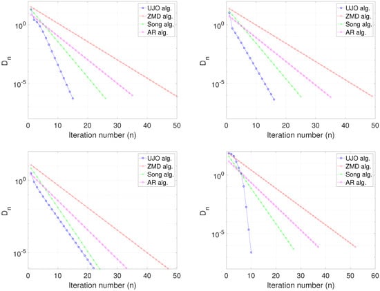
Let , where for all Let and be two mappings defined by
where We see that A is maximal monotone and B is a bounded linear operator. In addition, we define the mappings and by and for and Then, T and U are and -demigeneralized mappings, respectively, and demiclosed at zero. We choose Thus, our iterative scheme (17) becomes:
where Since the duality mappings () and reduce to the identity mappings on We compare the performance of (58) with the iterative scheme (6) of [9], (5) of [8] and (4) of [7]. For iteration (6), U is defined as above, which is 0-quasi-strict pseudocontractive mapping and . In addition, we take and For iteration (5), we consider the case for which and we take while,, for iteration (4), we choose We study the convergence of the algorithms using as a stopping criterion. We test the algorithms using the following initial values:
Case I:
Case II:
Case III:
Case IV:
Table 1.
Computation results for Example 1.
Figure 1.
Example 1, Top Left: Case I; Top Right: Case II; Bottom Left: Case III; Bottom Right: Case IV.
Example 2.
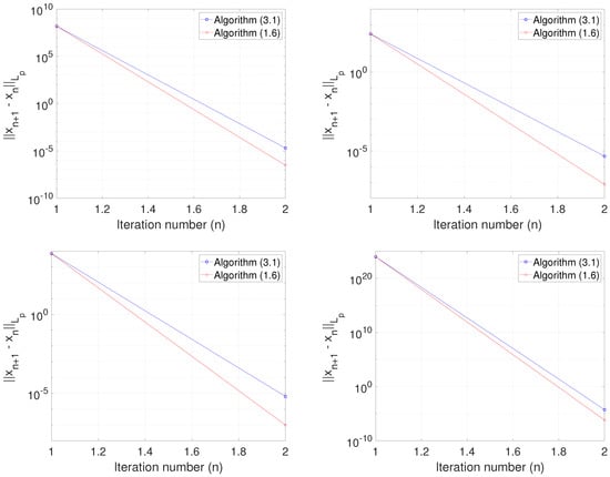
Next, we present an example in real Banach spaces. Let (for ) with norm and inner product for all Let The duality mapping is defined by (see [33])
Define the operator then, A is maximal monotone and the resolvent is the projection operator onto C which is given by
Furthermore, let Then, projection onto Q is given by
We set and then, T and U are -demigeneralized mappings. In addition, let be defined by for all In particular, we take so that E is not a real Hilbert space. We choose the following parameters and compare our method with the methods of Zi et al. [9] (Algorithm 1.6): For Algorithm 17, we take and, for Algorithm 1.6, we take We test the algorithms for the following initial values:
Case I:
Case II:
Case III:
Case IV:
Using , we plot the graphs of error against the number of iterations in each case. The computation results can be seen in Table 2 and Figure 2.
Table 2.
Computation results for Example 2.
Figure 2.
Example 2, Top Left: Case I; Top Right: Case II; Bottom Left: Case III; Bottom Right: Case IV.
Example 3.
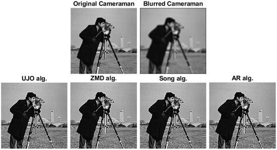
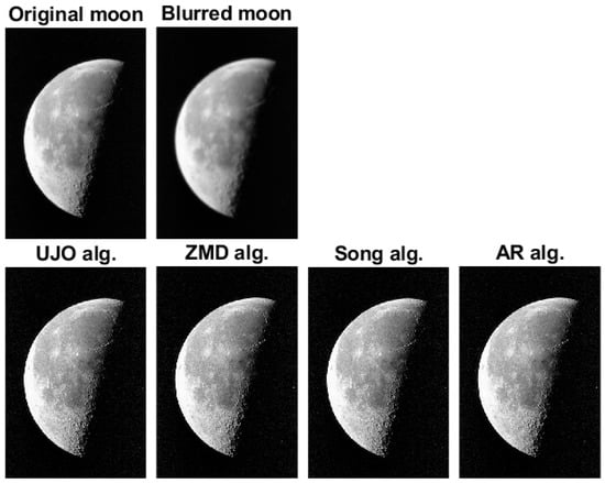
Next, we apply our result to solve the image restoration problem. We show the performance of our algorithm (17) with iteration (4)–(6). The image restoration problem can modeled as the linear system
where is the observed data with noisy, e is the noise, ( is a bounded linear operator, and is the vector with m non-zero components. This problem can also be formulated as the following Least Absolute Shrinkage and Selection Operator (LASSO) problem:
for some regularization parameter Equivalently, the split feasibility problem (1) can be rewritten as
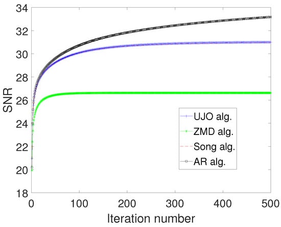
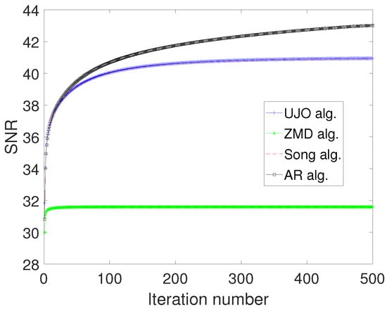
where and Following Corollary 1, we can apply our algorithm for solving the image deblurring problem by setting , , and , where In our experiments, we used the grey test image Cameraman () and Moon () in an Image Processing Toolbox in MATLAB, while each test image is degraded by Gaussian blur kernel with standard deviation In our computation, we take for (6), we take for (5), we take for (4), we take The maximum number of allowed iterations is set to be 1000. We compare the quality of the restored image using the signal-to-noise ratio defined as
where x is the original image and is the restored image. Typically, the larger the , the better the quality of the restored image. Figure 3 and Figure 4 show the reconstructed images using the iterative algorithms. In Figure 5 and Figure 6, we show the graphs of SNR against number of iterations for each algorithm. In Table 3, we show the time taken by each iteration for reconstruction of the test images.
Table 3.
Time (seconds) for computing the recovered images in Example 3.
5. Conclusions
In this paper, we introduced a new generalized explicit iterative method for solving generalized split feasibility problems in real Banach spaces. The algorithm is designed such that it is stepsize chosen self-adaptively and does not require the prior knowledge of the norm of the bounded linear operator, which is difficult to estimate in general. Furthermore, a strong convergence result is proved and some numerical examples are presented to illustrate the performance of the proposed method. In addition, the algorithm is applied to an image reconstruction problem to show its usefulness and efficiency.
Author Contributions
Conceptualization, L.O.J.; methodology, G.C.U. and L.O.J.; validation, G.C.U. and L.O.J.; formal analysis, G.C.U. and L.O.J.; writing—original draft preparation, G.C.U.; writing—review and editing, L.O.J. and C.C.O.; visualization, L.O.J.; supervision, G.C.U., L.O.J. and C.C.O.; project administration, G.C.U. and C.C.O.; funding acquisition, L.O.J. All authors approved the final manuscript. All authors have read and agreed to the published version of the manuscript.
Funding
This research was funded by the Sefako Makgatho Health Sciences University Postdoctoral research fund and the APC was funded by the Department of Mathematics and Applied Mathematics, Sefako Makgatho Health Sciences University, Pretoria, South Africa.
Institutional Review Board Statement
Not applicable.
Informed Consent Statement
Not applicable.
Data Availability Statement
Not applicable.
Acknowledgments
The authors acknowledge with thanks the Sefako Makgatho Health Sciences University for providing funds for the research. L.O.J. also thanks the the Federal University of Agriculture, Abeokuta, for hosting him and providing their facilities to support the course of the research.
Conflicts of Interest
The authors declare no conflict of interest. The funders had no role in the design of the study; in the collection, analyses, or interpretation of data; in the writing of the manuscript, or in the decision to publish the results.
References
- Censor, Y.; Elfving, T. A multiprojection algorithm using Bregman projection in a product splace. Numer. Algorithms 1994, 8, 221–239. [Google Scholar] [CrossRef]
- Byne, C. Iterative obligue projection onto convex sets and the split feasibility problem. Inverse Probl. 2002, 18, 441–453. [Google Scholar]
- Censor, Y.; Bortfeld, T.; Martin, B.; Trofimov, T. A unified approach for inversion problem in intensity-modolated radiation therapy. Phys. Med. Biol. 2006, 51, 2353–2365. [Google Scholar] [CrossRef] [Green Version]
- Censor, Y.; Elfving, T.; Kopf, N.; Bortfeld, T. The multiple-sets split feasibility problem and its applications. Inverse Probl. 2005, 51, 2071–2084. [Google Scholar] [CrossRef] [Green Version]
- Censor, Y.; Motova, A.; Segal, A. Pertured projections and subgradient projections for the multiple-sets split feasibility problems. J. Math. Anal. Appl. 2007, 327, 1244–1256. [Google Scholar] [CrossRef] [Green Version]
- Takahashi, W.; Xu, H.K.; Yao, J.C. Iterative methods for generalized split feasibility problems in Hilbert spaces. Set-Valued Var. Anal. 2014, 23, 205–221. [Google Scholar] [CrossRef]
- Ansari, Q.H.; Rehan, A. Iterative methods for generalized split feasibility problems in Banach spaces. Carp. J. Math. 2017, 33, 9–26. [Google Scholar] [CrossRef]
- Song, Y. Iterative methods for fixed point problems and generalized split feasibility problems in Banach spaces. J. Nonlinear Sci. Appl. 2018, 11, 198–217. [Google Scholar] [CrossRef] [Green Version]
- Zi, X.; Ma, Z.; Du, W.S. Strong convergence theorems for generalized split feasibility problems in Banach spaces. Mathematics 2020, 8, 892. [Google Scholar] [CrossRef]
- Zhao, J. Solving split equality fixed-point problem of quasi-nonexpansive mappings without prior knowledge of operators norms. Optimization 2015, 64, 2619–2630. [Google Scholar] [CrossRef]
- Ke, Y.; Ma, C. The generalized viscosity implicit rules of nonexpansive mappings in Hilbert space. Fixed Point Theory Appl. 2015, 2015, 190. [Google Scholar] [CrossRef] [Green Version]
- Hoffman, J.D. Numerical Methods for Engineers and Scientists, 2nd ed.; Marcel Dekker, Inc.: New York, NY, USA, 2001. [Google Scholar]
- Palais, R.S.; Palais, R.A. Differential Equations, Mechanics, and Computation; American Mathematical Society: Providence, RI, USA, 2009. [Google Scholar]
- Marino, G.; Scardamaglia, B.; Zaccone, R. A general viscosity explicit midpoint rule for quasi-nonexpansive mappings. J. Nonlinear Convex Anal. 2017, 18, 137–148. [Google Scholar]
- Xu, H.K. Inequalities in Banach spaces with applications. Nonlinear Anal. 1991, 16, 1127–1138. [Google Scholar] [CrossRef]
- Cioranescu, I. Geometry of Banach Spaces, Duality Mappings and Nonlinear Problems; Kluwer Academic: Dordrecht, The Netherlands, 1990. [Google Scholar]
- Reich, S. A weak convergence theorem for the alternating method with Bregman distance. In Theory and Applications of Nonlinear Operators of Accretive and Monotone Type; Kartsatos, A.G., Ed.; Marcel Dekker: New York, NY, USA, 1996; pp. 313–318. [Google Scholar]
- Takahashi, W. Nonlinear Functional Analysis; Yokohama Publishers: Yokohama, Japan, 2000. [Google Scholar]
- Nilsrakoo, W.; Saejung, S. Strong convergence theorems by Halpern-Mann iterations for relatively nonexpansive maps in Banach spaces. Appl. Math. Comput. 2011, 217, 6577–6586. [Google Scholar] [CrossRef]
- Matsushita, S.; Takahashi, W. A strong convergence theorem for relatively nonexpansive mappings in Banach spaces. J. Approx. Theory 2005, 134, 257–266. [Google Scholar] [CrossRef] [Green Version]
- Alber, Y.I. Metric and generalized projection operators in Banach spaces: Properties and applications. In Theory and Applications of Nonlinear Operators of Accretive and Monotone Type; Kartsatos, A.G., Ed.; Lecture Notes Pure Appl. Math.; Dekker: New York, NY, USA, 1996; Volume 178, pp. 15–50. [Google Scholar]
- Alber, Y.I.; Guerre-Delabriere, S. On the projection methods for fixed point problems. Analysis 2001, 21, 17–39. [Google Scholar] [CrossRef]
- Alber, Y.I.; Reich, S. An iterative method for solving a class of nonlinear operator equations in Banach spaces. Panamer. Math. J. 1994, 4, 39–54. [Google Scholar]
- Zhou, H.; Gao, E. An iterative method of fixed points for closed and quasi-strict pseudocontractions in Banach spaces. J. Appl. Math. Comput. 2010, 33, 227–237. [Google Scholar] [CrossRef]
- Takahashi, W.; Wen, C.F.; Yao, J.C. Strong convergence theorem by shrinking projection method for new nonlinear mappings in Banach spaces and applications. Optimization 2017, 66, 609–621. [Google Scholar] [CrossRef]
- Browder, F.E. Browder, Nonlinear maximal monotone operators in a Banach space. Math. Ann. 1968, 175, 89–113. [Google Scholar] [CrossRef] [Green Version]
- Kamimura, S.; Takahashi, W. Strong convergence of a proximal-type algorithm in a Banach space. SIAM J. Optim. 2002, 13, 938–945. [Google Scholar] [CrossRef]
- Kohsaka, F.; Takahashi, W. Strong convergence of an iterative sequence for maximal monotone operators in a Banach space. Abstr. Appl. Anal. 2004, 2004, 239–249. [Google Scholar] [CrossRef] [Green Version]
- Khan, A.R.; Ugwunnadi, G.C.; Makukula, Z.G.; Abbas, M. Strong convergence of inertial subgradient extragradient method for solving variational inequality in Banach space. Carpathian J. Math. 2019, 35, 327–338. [Google Scholar] [CrossRef]
- Xu, H.K. Iterative algorithms for nonlinear operators. J. Lond. Math. Soc. 2002, 66, 240–256. [Google Scholar] [CrossRef]
- Maingé, P.E. Strong convergence of projected subgradient methods for nonsmooth and nonstrictly convex minimization. Set-Valued Anal. 2008, 16, 899–912. [Google Scholar] [CrossRef]
- Rockafellar, R.T. On the maximality of sums of nonlinear monotone operators. Trans. Am. Math. Soc. 1970, 149, 75–88. [Google Scholar] [CrossRef]
- Agarwal, R.P.; Regan, D.O.; Sahu, D.R. Fixed Point Theory for Lipschitzian-Type Mappings with Applications; Springer: Berlin/Heidelberg, Germany, 2009. [Google Scholar]
Publisher’s Note: MDPI stays neutral with regard to jurisdictional claims in published maps and institutional affiliations. |
© 2022 by the authors. Licensee MDPI, Basel, Switzerland. This article is an open access article distributed under the terms and conditions of the Creative Commons Attribution (CC BY) license (https://creativecommons.org/licenses/by/4.0/).