A Peek Outside Our Universe

Abstract

According to general relativity (GR), a universe with a cosmological constant $\Lambda$, like ours, is trapped inside an event horizon, $r<\sqrt{3/\Lambda }$. What is outside? We show, using Israel (1967) junction conditions, that there could be a different universe outside. Our universe looks like a black hole for an outside observer. Outgoing radial null geodesics cannot escape our universe, but incoming photons can enter and leave an imprint on our CMB sky. We present a picture of such a fossil record from the analysis of CMB maps that agrees with the black hole universe predictions but challenges our understanding of the origin of the primordial universe.

1. Introduction

An event horizon (EH) $r_{*}$, or trapped surface, for a given observer can be defined as the distance beyond which this observer will never see: $r<r_{*}$. The most famous EH is, of course, that of a black hole (BH) of mass M. Dimensional analysis tells us that a relativistic (c) gravitational (G) system of mass M has an associated EH: $r_{*}\simeq GM/c^2$. The same dimensional analysis indicates that a cosmological constant $\Lambda$ is associated with a relativistic EH, $r_{*}\simeq 1/\sqrt{\Lambda c^2}$, which, in principle, is independent of G. We will show first how these EHs appear as solutions to Einstein’s field equations and next how the different EHs are related in our universe expansion.

The most general form for a metric with spherical symmetry in proper coordinates $x^{\mu }=(t,r,\delta ,\theta )$ with $c=1$ can be written as [1]:

$$d{s}^2=g_{\mu \nu }d{x}^{\mu }d{x}^{\nu }=-A(t,r)d{t}^2+B(t,r)d{r}^2+r^{2}d{\Omega }^2$$

(1)

where we have introduced: $d{\Omega }^2={cos}^2\delta d{\theta }^2+d{\delta }^2$. Einstein’s field equations for that metric in empty space $\rho =p=\Lambda =0$ result in the Schwarzschild (SW) metric:

$$d{s}^2=-[1-\frac{2GM}{r}]d{t}^2+\frac{d{r}^2}{1-\frac{2GM}{r}}+r^{2}d{\Omega }^2$$

(2)

where M can be interpreted as a singular point mass at $r=0$. As it is well known, the EH at $r_{*}=2GM$ prevents us from seeing such a naked singularity [2]. Outgoing null radial geodesics cannot leave the interior of $r_{*}$, whereas incoming null radial geodesics can cross inside $r_{*}$ in proper time, even when, for an observer outside, this takes $t=\infty$ in her time.

1.1. deSitter Metric

The solution for Equation (1) with $\rho =p=M=0$ but $\Lambda \ne 0$ is the deSitter (dS) metric:

$$d{s}^2=-[1-r^2{H}_{\Lambda }^2]d{t}^2+\frac{d{r}^2}{1-r^2{H}_{\Lambda }^2}+r^{2}d{\Omega }^2$$

(3)

which is also static and has an EH, or trapped surface, at $r_{*}=1/H_{\Lambda }$, where $H_{\Lambda }^2\equiv 8\pi G{\rho }_{\Lambda }/3$ and ${\rho }_{\Lambda }=\Lambda /\left(8\pi G\right)+{\rho }_{vac}$. We include a constant ${\rho }_{vac}=V=V\left(\varphi \right)=-p_{vac}$ to account for vacuum energy (or the potential of a trapped scalar field), which is physically degenerate with $\Lambda$. The inside of $r_{*}=1/H_{\Lambda }$ is causally disconnected and corresponds to an EH: radial null events ($d{s}^2=0$) connecting $(0,r_0)$ with $(t,r)$ take $t=\infty$ to reach $r=r_{*}$ from any point inside.

1.2. The FLRW Metric and $\Lambda$

The Friedmann–Lemaitre–Robertson–Walker (FLRW) flat ($k=0$) metric in spherical comoving coordinates $(\tau ,\chi ,\delta ,\theta )$, corresponds to a homogeneous and isotropic space-time:

$$d{s}^2=-d{\tau }^2+a{\left(\tau \right)}^2\left[d{\chi }^2+{\chi }^{2}d{\Omega }^2\right]$$

(4)

where the scale factor $a\left(\tau \right)$ describes the expansion/contraction as a function of time. For a comoving observer and a perfect fluid, the field equations reduce to:

$$3H^2\equiv 3{\left(\frac{\dot{a}}{a}\right)}^2=8\pi G({\rho }_m{a}^{-3}+{\rho }_R{a}^{-4}+{\rho }_{\Lambda })$$

(5)

where ${\rho }_m$ and ${\rho }_R$ are the matter and radiation density today ($a=1$) and ${\rho }_{\Lambda }=-p_{\Lambda }$ is the effective cosmological constant density introduced in the dS metric. Given $\rho$ and p at some time, we can find $a=a\left(\tau \right)$ and determine the metric in Equation (4). Observations show that the expansion rate today is dominated by ${\rho }_{\Lambda }$. This indicates that the FLRW metric describes the interior of a trapped surface of size $r_{*}=1/H_{\Lambda }$, like the dS metric. In fact, both metrics are equivalent in that regime [3,4]. They also reproduce the steady-state cosmological principle [5].

Interpreting $\Lambda$ as a boundary term to the GR equations and imposing the so-called zero action principle, $r_{*}=1/H_{\Lambda }$ can be given in terms of ordinary contributions to the energy density, ${\rho }_{\Lambda }=<{\rho }_m/2+{\rho }_R>$ [6,7].

1.3. SW–FLRW Perturbation

The Schwarzschild (SW) metric is commonly used to describe the outside of BHs or stars and it should be understood as a perturbation inside a larger background. An example of this is the Schwarzschild–deSitter (SW–dS) metric:

$$d{s}^2=-[1-\frac{2GM}{r}-r^2{H}_{\Lambda }^2]d{t}^2+\frac{d{r}^2}{1-\frac{2GM}{r}-r^2{H}_{\Lambda }^2}+r^{2}d{\Omega }^2$$

(6)

which corresponds to an exact solution with both non-zero $\Lambda$ and M. More generally, the FLRW metric is the background to the SW solution [8], e.g., it replaces $r=a\left(\tau \right)\chi$ in Equation (2). For large r, we recover the dS metric, as in Equation (6) above, which is equivalent to the FLRW metric dominated by $\Lambda$ [3]. Close to the BH at $r_{*}<r<1/H_{\Lambda }$, we recover the SW metric.

2. Outside Our FLRW Universe

In proper coordinates $r=a\chi$, the FLRW metric with $H=H\left(\tau \right)$ is also trapped inside the same EH as the dS metric, $r_{*}=1/H_{\Lambda }$, because $H\left(\tau \right)>H_{\Lambda }$. We can see this by considering outgoing radial null geodesics in the FLRW metric (Equation (4)):

$$r_{out}=a\left(\tau \right){\int }_{\tau }^{\infty }\frac{d{\tau }^{\prime }}{a\left({\tau }^{\prime }\right)}=a{\int }_a^{\infty }\frac{dln{a}^{\prime }}{a^{\prime }H\left(a^{\prime }\right)}<\frac{1}{H_{\Lambda }}=r_{*}$$

(7)

which shows that signals cannot escape from the inside to the outside of the EH. However, incoming radial null geodesics $a\left(\tau \right){\int }_0^{\tau }\frac{d\tau }{a\left(\tau \right)}$ could be larger than $r_{*}$ if we look back in time long enough. This shows that observers living in the interior are trapped inside the EH, but they can, in principle, observe what happened outside.

What is outside $r_{*}=1/H_{\Lambda }$ in the FLRW metric? The FLRW comoving coordinates $(\tau ,\chi )$ can be matched to the SW proper coordinates $(t,r)$. The joint metric is what [4,6] call a BHU solution. The particular case where the inside is dS (and the outside SW) is called BH.fv (where fv stands for false vacuum). The BHU metric is also a solution to Einstein’s field equations. To prove this, we simply need to show that the junction follows the Israel matching conditions [9]. The two metrics can be matched on a timelike hypersurface $\Sigma$ of constant $\chi$:

$$d{s}_{\Sigma }^2=h_{ab}d{y}^{a}d{y}^b=-d{\tau }^2+a^2\left(\tau \right){\chi }_{\S }^{2}d{\Omega }^2$$

(8)

and the extrinsic curvature K at $\Sigma$ is the same in both sides. The matching conditions $h_{-}=h_{+}$ and $K_{+}=K_{-}$ reduce to [4]

$$r=R\left(\tau \right)=a\left(\tau \right){\chi }_{\S };{\dot{R}}^2=R^2{H}^2=\frac{R_{*}}{R}$$

(9)

where $R_{*}\equiv 2GM$. Staring from small a, as we increase $\tau$, both R and $\dot{R}=HR$ grow until we reach $HR=c=1$, which corresponds to the event horizon $R_{*}=2GM=1/H_{\Lambda }$. It takes $t=\infty$ in SW time to asymptotically reach $R_{*}$. This proves that the joint BHU metric is also a solution to Einstein’s field equations with no surface terms in the junction. This is equivalent to stating that the $\Lambda$ term corresponds to a trapped surface $R_{*}=1/H_{\Lambda }$ in the FLRW metric which matches the EH of a BH. Generalization to $k\ne 1$ is straightforward (see §12.5.1 in [1,4,10]).

Recall that the SW metric is a perturbation of a larger FLRW metric, i.e, a BH-like metric embedded in a background described by the FLRW metric. This means that outside $r_{*}=1/H_{\Lambda }$, we have another FLRW metric, like in a Matryoshka doll. From the outside, the inner FLRW metric looks like a BH. There could be many other BHUs inside and outside $r_{*}=1/H_{\Lambda }$, so the structure could be better described by a fractal.

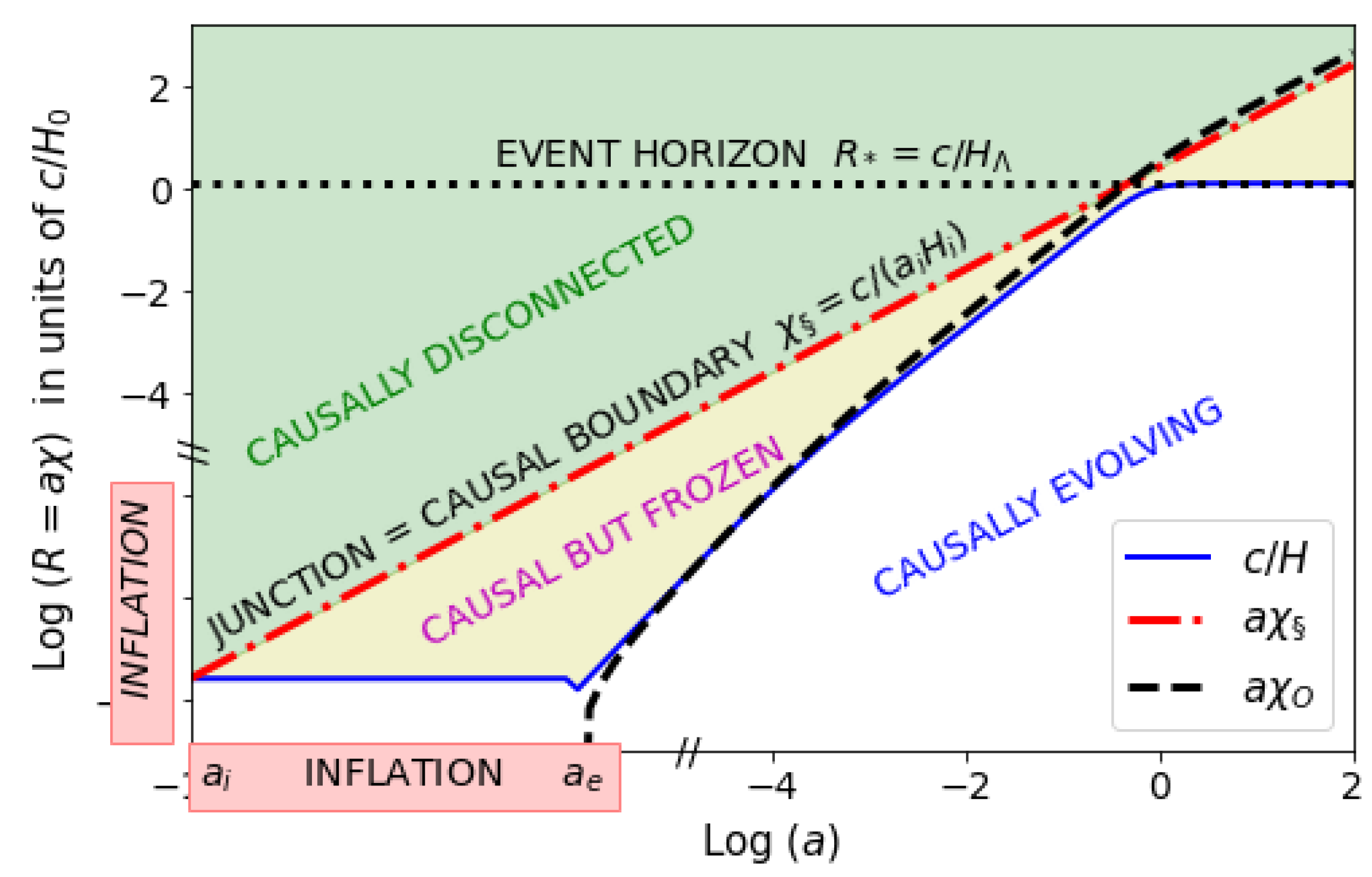
2.1. Causal Structure

In the FLRW universe, the Hubble horizon $r_H$ is defined as $r_H=c/H$. Scales larger than $r_H$ cannot evolve because the time a perturbation takes to travel that distance is larger than the expansion time. This means that $r>r_H$ scales are "frozen out" (structure cannot evolve) and are causally disconnected from the rest. Thus, $c/H$ represents a dynamical causal horizon that is evolving (blue line in Figure 1).

Figure 1. Proper coordinate: $R=a\left(\tau \right)\chi$ in units of $c/H_0$ as a function of cosmic time a. The Hubble horizon $c/H$ (blue continuous line) is compared to the observable universe $a{\chi }_O$ after inflation (dashed line) and the primordial causal boundary ${\chi }_{\S }=c/\left(a_i{H}_i\right)$ (dot-dashed red line). Larger scales (green shading) are causally disconnected and smaller scales (yellow shading) are dynamically frozen. After inflation, $c/H$ grows again. At $a\simeq 1$, the Hubble horizon reaches our event horizon $R_{*}=c/H_{\Lambda }$. At the CMB last scattering, we can observe both frozen and causally disconnected perturbations.

We can sketch the evolution of our universe in Figure 1. A primordial field $\psi$ settles or fluctuates into a false (or slow-rolling) vacuum which will create a BH.fv with a junction $\Sigma$ in Equation (8), where the causal boundary is fixed in comoving coordinates and corresponds to the particle horizon during inflation, ${\chi }_{\S }=c/\left(a_i{H}_i\right)$, or the Hubble horizon when inflation begins. The size $R=a\left(\tau \right){\chi }_{\S }$ of this vacuum grows and asymptotically tends to $R_{*}=c/H$ following Equation (9) with $H=H_i$. The inside of this BH will be expanding exponentially, $a=e^{\tau H_i}$, while the Hubble horizon is fixed at $1/H_i$. When this inflation ends [11,12,13,14], vacuum energy excess converts into matter and radiation (reheating). This results in BHU, where the infinitesimal Hubble horizon starts to grow following the standard Big Bang evolution. The observable universe (or particle horizon) after inflation, ${\chi }_O$, is:

$${\chi }_O={\chi }_O\left(a\right)={\int }_{a_e}^a\frac{dln{a}^{\prime }}{a^{\prime }H\left(a^{\prime }\right)}={\chi }_O\left(1\right)-\overline{\chi }\left(a\right),$$

(10)

where $a_e$ is the scale factor when inflation ends. For ${\Omega }_{\Lambda }\simeq 0.7$, the particle horizon today is ${\chi }_O\left(1\right)\simeq 3.26c/H_0$ and $\overline{\chi }\left(a\right)={\int }_a^{1}dlna/\left(aH\right)$ is the radial lookback time, which, for a flat universe, agrees with the comoving angular diameter distance, $d_A=\overline{\chi }$. The observable universe becomes larger than $R_{*}$ when $a>1$, as shown in Figure 1 (compare dotted and dashed lines). This shows that observers like us, living in the interior of the BH universe, are trapped inside $R_{*}$ but can nevertheless observe what happened outside. We can estimate ${\chi }_{\S }$ from ${\rho }_{\Lambda }=<{\rho }_m/2+{\rho }_R>$ (see §I.A), where the average is in the lightcone inside ${\chi }_{\S }$. For ${\Omega }_{\Lambda }\simeq 0.7$,6] found that ${\chi }_{\S }\simeq 3.34c/H_0$, which is close to ${\chi }_O$ today. Imagine that ${\Omega }_{\Lambda }$ is caused by some dark energy and has nothing to do with ${\chi }_{\S }$. We still have that ${\chi }_{\S }\lesssim {\chi }_O$, because otherwise ${\chi }_{\S }$ would have crossed $RH=1$ early on, resulting in a smaller ${\chi }_O$ than measured (see Figure 1).

Thus, at the time of the CMB last scattering (when $d_A\simeq {\chi }_O$), ${\chi }_{\S }$ corresponds to an angle $\theta ={\chi }_{\S }/d_A\lesssim 1$rad$\simeq 60$ deg. Therefore, we can actually observe scales larger than ${\chi }_{\S }$, scales that are not causally connected! This could be related to the so-called CMB anomalies (i.e, apparent deviations with respect to simple predictions from $\Lambda$CDM, see [15,16] and references therein) or the parameter tensions in measurements from vastly different cosmic scales or times [17,18,19,20]).

2.2. A Peek Outside

A recent analysis of the Planck temperature anisotropy data, Ref. [21], shows that the distribution of best-fit dark energy density ${\Omega }_{\Lambda }$ exhibits three distinct regions across the CMB sky (marked by the three large grey circles in Figure 2). These regions have radii ranging from 40 to 70 degrees. The sizes of these structures are in agreement with the scale of the causal boundary ${\chi }_{\S }$ for $\Lambda$ dominated universes. As shown in [21], the size of each of these regions is correlated with the mean value of ${\Omega }_{\Lambda }$ over that portion of the sky, in good agreement with the BHU prediction. The same large-scale anisotropic patterns are observed for the distribution of other basic $\Lambda$CDM cosmological parameters. This represents a very significant break-down of the main hypothesis of the Big Bang model: the assumption that the universe is isotropic on a large scale. The observed anisotropy has a tiny probability (of order ${10}^{-9}$) of being a Gaussian statistical fluctuation of an otherwise isotropic universe [21].

Figure 2. Map of the best-fit values of the dark energy density ${\Omega }_{\Lambda }$ across the celestial sphere, estimated from partial sky (discs) measurements of the Planck CMB maps. The large grey circles delimit areas across the sky with significantly different values of ${\Omega }_{\Lambda }$.

In summary, Figure 2 shows that: (a) regions with a given value of ${\Omega }_{\Lambda }$ have a corresponding angular size $\theta$ that agrees with the BHU prediction (see Figure 31 in [21]), (b) causally disconnected regions of the sky (larger than ${\chi }_{\S }$) fit the same physical model of acoustic oscillations very well, and (c) the background is similar but with parameters that are significantly different across disconnected regions. This suggests that the underlying physical mechanism sourcing the observed anisotropy encompasses scales beyond our causal universe. This is in apparent tension with simple models of inflation (as sources of perturbation for the largest scales) and opens the door to revisiting our basic understanding of the origin of the primordial universe.

References

- Padmanabhan, T. Gravitation: Foundations and Frontiers; Cambridge University Press: Cambridge, UK, 2010. [Google Scholar]
- Penrose, R. Gravitational Collapse: The Role of General Relativity. Nuovo Cimento Rivista Serie 1969, 1, 252. [Google Scholar]
- Mitra, A. Interpretational conflicts between the static and non-static forms of de Sitter metric. Sci. Rep. 2012, 2, 923. [Google Scholar] [CrossRef] [PubMed] [Green Version]
- Gaztanaga, E.D. The Black Hole Universe (BHU) from a FLRW Cloud. Submitted to Physics of the Dark Universe. Available online: https://hal.archives-ouvertes.fr/hal-03344159 (accessed on 14 September 2021).
- O’Raifeartaigh, C.; Mitton, S. A new perspective on steady-state cosmology. arXiv 2015, arXiv:1506.01651. [Google Scholar]
- Gaztañaga, E. The cosmological constant as a zero action boundary. Mon. Not. R. Astron. Soc. 2021, 502, 436–444. [Google Scholar] [CrossRef]
- Gaztanaga, E. The size of our causal Universe. Mon. Not. R. Astron. Soc. 2020, 494, 2766–2772. [Google Scholar] [CrossRef] [Green Version]
- Kaloper, N.; Kleban, M.; Martin, D. McVittie’s legacy: Black holes in an expanding universe. Phys. Rev. D 2010, 81, 104044. [Google Scholar] [CrossRef] [Green Version]
- Israel, W. Singular hypersurfaces and thin shells in general relativity. Nuovo Cimento B Serie 1967, 48, 463. [Google Scholar] [CrossRef] [Green Version]
- Stuckey, W.M. The observable universe inside a black hole. Am. J. Phys. 1994, 62, 788–795. [Google Scholar] [CrossRef]
- Starobinskiǐ, A.A. Spectrum of relict gravitational radiation and the early state of the universe. Sov. Exp. Theor. Phys. Lett. 1979, 30, 682. [Google Scholar]
- Guth, A.H. Inflationary universe: A possible solution to the horizon and flatness problems. Phys. Rev. D 1981, 23, 347–356. [Google Scholar] [CrossRef] [Green Version]
- Linde, A.D. A new inflationary universe scenario: A possible solution of the horizon, flatness, homogeneity, isotropy and primordial monopole problems. Phys. Lett. B 1982, 108, 389–393. [Google Scholar] [CrossRef]
- Albrecht, A.; Steinhardt, P.J. Cosmology for Grand Unified Theories with Radiatively Induced Symmetry Breaking. Phys. Rev. Lett. 1982, 48, 1220–1223. [Google Scholar] [CrossRef]
- Planck Collaboration. Planck 2018 results. VII. Isotropy and statistics of the CMB. Astron. Astrophys. 2020, 641, A7. [Google Scholar] [CrossRef] [Green Version]
- Schwarz, D.J.; Copi, C.J.; Huterer, D.; Starkman, G.D. CMB anomalies after Planck. Class. Quantum Gravity 2016, 33, 184001. [Google Scholar] [CrossRef]
- Planck Collaboration. Planck 2018 results. VI. Cosmological parameters. Astron. Astrophys. 2020, 641, A6. [Google Scholar] [CrossRef] [Green Version]
- Riess, A.G. The expansion of the Universe is faster than expected. Nat. Rev. Phys. 2019, 2, 10–12. [Google Scholar] [CrossRef] [Green Version]
- DES Collaboration. Cosmological Constraints from Multiple Probes in the Dark Energy Survey. Phys. Rev. Lett. 2019, 122, 171301. [Google Scholar] [CrossRef] [PubMed] [Green Version]
- Di Valentino, E.; Mena, O.; Pan, S.; Visinelli, L.; Yang, W.; Melchiorri, A.; Mota, D.F.; Riess, A.G.; Silk, J. In the realm of the Hubble tension-a review of solutions. Class. Quantum Gravity 2021, 38, 153001. [Google Scholar] [CrossRef]
- Fosalba, P.; Gaztañaga, E. Explaining cosmological anisotropy: Evidence for causal horizons from CMB data. Mon. Not. R. Astron. Soc. 2021, 504, 5840–5862. [Google Scholar] [CrossRef]
Publisher’s Note: MDPI stays neutral with regard to jurisdictional claims in published maps and institutional affiliations. |
© 2022 by the authors. Licensee MDPI, Basel, Switzerland. This article is an open access article distributed under the terms and conditions of the Creative Commons Attribution (CC BY) license (https://creativecommons.org/licenses/by/4.0/).