Abstract
As a test of the time symmetry of forbidden-line emission processes, we measured the [OIII]4959 and 5007 emission lines of more than 12,000 galaxies from the Sloan Digital Sky Survey DR8 to examine the [OIII]4959,5007 flux ratio as a function of redshift z. Using two different approaches, we fitted each line with a Gaussian curve and rejected any spectrum not conforming to requirements of line symmetry, S/N levels, and continuum fit. We found the variance in the ratio of flux to be between 4.7 and −3.3% for which is consistent with no change. After correcting for systematic effects of noise, we found the mean value of the [OIII]4959,5007 flux ratio to be 2.98 ± 0.01 which is consistent with theory and previous studies using AGN spectra. We also used these data to estimate an upper limit on the time dependence of the fine structure constant of / for galaxies within the same redshift range. This corresponds to yr, which is also in line with previous estimates from SDSS QSO data.
1. Introduction
A prominent emission doublet in the spectra of nearly all photoionized nebulae is the forbidden line doublet of [OIII]4960.295 Å (2s2pD-2s2pP) and 5008.239 Å (2s2pD-2s2pP) (hereafter referred to as 4959 and 5007, respectively; the listed wavelengths are for a vacuum). These two particular spectral lines are produced by magnetic dipole interactions with a small contribution of electric quadrupole radiation [1,2].
The absolute strengths of the 4959 and 5007 lines are a function of the local conditions within the radiating nebula, such as temperature, radiation flux, and ion number density [3]. At temperatures typical for average HII regions, the [OIII]4959,5007 doublet is present with both lines being weaker than that of H. However, within significantly hot nebulae containing a harder ionizing flux, such as planetary nebulae, the 5007 line can be considerably stronger than the H line. Even so, the ratio of the 5007 and 4959 line flux, which we designate as , is not dependent upon upon local effects since both transitions originate from the same 2s2p level of this ion. Their relative strengths are determined by the probability of the electron transitioning down to either the (2s2pP) level or the (2s2pP) level, which is in turn determined solely by the atomic properties of the O ion.
A significant amount of theoretical work has been performed to determine , deducing values ranging from 2.89 to 3.03 [1].Taking the relativistic effects of the magnetic dipole operator into account gives a theoretical ratio value of 2.98 [4]. An observational analysis using high S/N spectra from 62 AGN obtained a value of = 2.993 ± 0.014, which agrees with the aforementioned theoretical value [2]. Based on these most recent works, a value of 2.98 is commonly taken to be the best estimate of the true value.
It is reasonable to assume that is constant and unchanging in time, but it is worth reviewing some of the published literature supporting or challenging this. (We refer the reader to the excellent presentation of Uzan [5] for a more extensive review). The energy differences from the atomic transitions giving rise to the 4959,5007 lines include fundamental constants such as the charge of the electron and the speed of light [1]. A possible deviation with redshift of the fine structure constant , which is a function of the electron charge, Planck’s constant, and the speed of light, has been inferred from QSO absorption lines [6,7,8]. It has been proposed that “running vacuum models” of the universe that allow fundamental constants to vary with the Hubble parameter fit basic cosmological observational data better than standard Cold Dark Matter (CDM) models [9]. Other models of the universe that allow for variation in fundamental constants include minisuperspace models [10], inhomogeneous pressure models [11], and cyclic universe & alternate gravity models [12].
Most evidence, however, supports the fundamental constants of nature remaining unchanged over measurable time. Studies of the Oklo natural fission reactor place an upper limit on / of over the last 2 Gyrs [13]. Studies of QSO spectra specifically using measured wavelengths of the [OIII]4959,5007 doublet find / to be less than over the last ∼8 Gyr [14,15,16,17]. Theoretical studies of CDM models that allow the cosmological constant to vary, constrain / to be less than [18]. In fact any significant variation in only exacerbates the fine-tuning problem of the vacuum energy [19]. Studies of absorption lines in distant QSOs constrain / to be less than [20]. Studies performed on gravitational lensing [21], the cosmic microwave background (CMB), and the Lyman- forest [22] constrain / to be less than 10 (0.075 < z < 2.269), 10 (z ∼ 1100), and 10 (z < 6), respectively. An analysis of data from numerous independent sources including type Ia supernovae, quasars, atomic clocks, the CMB, and big bang nucleosynthesis place constraints on / ranging from 10 to 10, with all sources having a range in redshift of 0.3 < z < 4.2 [23,24]. All of these derived constraints are consistent with no variation at all.
Even if there were evidence for variability in fundamental constants, we note that has only a weak dependence on such constants. Factors determining emission strength such as the speed of light, the permittivity of space, and the charge on the electron, essentially divide out in the ratio, reducing it to the simplified formula
where A represents the Einstein A coefficient for the specified emission. This coefficient can be defined as
Here, and represent the matrix dipole element and frequency of the transition, represents the degeneracy of the nth level, and represents the greater value of the degeneracies for n or n. Thus factors such as the degeneracy degrees and matrix dipole operators of the levels within the transitions have a greater bearing on the ratio value than universal constants. Examining the z dependence of is then essentially a test of the time symmetry of the O ion itself.
Encouraged by the available number of published galaxian spectra as a function of z, we determined to see if there is evidence that has changed over time. In Section 2 we discuss our data, the analysis used to calculate the ratio, and the results. In Section 3 we derive an estimate of . In Section 4 we discuss our conclusions.
2. Data and Methods
We obtained a list of galaxies with [OIII]4959,5007 emission from Sloan Digital Sky Survey Data Release 8 (SDSS DR8) from the online file galSpecLine-dr8.fits available at https://www.sdss.org/dr12/spectro/galaxy_mpajhu/ (accessed on 25 January 2022). All spectra were flux and wavelength calibrated according to standard prescriptions [25]. Each tabulated galaxy spectrum had been processed through the Max Planck Institute for Astrophysics and the Johns Hopkins University spectroscopic parameters pipeline and had emission-line measurements given in units of erg cm s Å. Unreliable or absent measurements were flagged in the file for easy removal. In all, 22,389 spectra were listed within the redshift range of 0 < z < 0.7, including duplicated spectra. The tabulated emission-line parameters, reasonably accurate for the studies of star formation, stellar mass, and oxygen abundances for which they were intended, were deprecated in favor of a reanalysis by a team from Wisconsin, Portsmouth, and Granada of data from DR12 [26].
We determined through manual measurements using IRAF that more accurate values for the 4959 and 5007 emission-line fluxes could be obtained, largely through more precisely locating the continuum around these specific lines. We therefore remeasured all line fluxes with software written specifically for the 5007,4959 lines.
2.1. First Analysis
The total emission flux for a given line was estimated from curves fitted to the line profile. The specific profiles examined for appropriateness of fit were Gaussian, Lorentzian, Voigt, and Moffat. To start, each of these, as well as a sum of the Gaussian and Moffat profiles, were fit to the [OIII] lines of each spectrum in the data set. We found that, as expected, the Gaussian profile provided the greatest number of instances where the algorithm converged and also gave the smallest average sum-squared error of the fits. Therefore, we used a Gaussian profile exclusively.
We wrote a fitting algorithm in Python using the method inside the Scipy optimize package, which is based on non-linear least-squares fitting. Values of the centroid and line width of the H, 4959, and 5007 lines in each spectrum were estimated from their peak value and FWHM, respectively, and used to seed the algorithm. The algorithm returned a resultant line amplitude, line width, line center, and continuum value.
Correctly estimating the continuum beneath the emission lines was critical in determining their true flux. As a first attempt, we applied a linear fit between the continuum 20 Å to 50 Å redward of 5007 and 20 Å to 50 Å blueward of H as measured in the rest frame. We chose these particular wavelength ranges to avoid contamination from all but the broadest H emission-line wings. Spectra with H emission broad enough to affect the fit were removed from the data set.
We then created an index which we referred to as the “continuum color” to estimate the continuum slope through the emission lines. This index was the mean of the blueward continuum values minus the mean of the redward values divided by their sum, with more positive values indicating a bluer continuum. We found a strong correlation between continuum color and ratio, confirming that a linear fit was inappropriate.
To address this problem we adopted a two-stage process. After fitting the emission lines, we subtracted their fit from each spectrum. We then fit the 188 Å range from 70 Å blueward of 4959 to 70 Å redward of 5007 in the residual spectrum, again as measured in the rest frame. The data in this range was fitted with a third-order Legendre polynomial. This fit was then subtracted from the original spectrum and the 5007 and 4959 lines were again fitted with Gaussian profiles. These second fits were integrated over the emission lines and the small residual flux from the continuum offset was subtracted off. The ratio was then obtained by dividing the 5007 flux counts by the 4959 flux counts.
2.2. Spectrum Evaluation
At the linear continuum fitting stage we rejected spectra which had steeply-sloped continua for fear that these could not be properly continuum subtracted. At this and the subsequent Legendre polynomial continuum fitting stage we rejected spectra if the fit returned a width of either line in excess of 30 Å. As previously noted, this was to avoid broad emission in general since it tended to confuse continuum subtraction. Spectra were also rejected if the amplitude of the 5007 emission line was less than 50 flux counts to avoid lines with low S/N. Spectra having nonphysical values from misfitting, such as negative line fluxes or flux values of the 4959 emission line which were greater than that of the 5007 emission line, were also rejected. Finally, spectra having an amplitude of either emission line that exceeded 1000 flux counts were rejected to cautiously guard against detector non-linearity.
To avoid giving the computer algorithm an exclusive final say, we reviewed each spectrum individually by eye to ensure that all fits were reasonable. To do this four plots were generated. The first showed the full spectrum without any fits. The second showed the 188 Angstroms of the spectrum centered around the [OIII] lines, with the linear continuum fit overlaid. The third and fourth plots showed the 5007 and 4959 emission lines, respectively, overlaid with their Gaussian and local continuum fits.
To preserve objectivity, the calculated ratios, as well as the redshift, were hidden from the reviewer so that the visual analysis was based only on the appropriateness of the continuum and emission-line fits. A spectrum was removed from the data set at this stage if it met one or more of the following criteria: (1) the Gaussian fit on either emission line clearly did not match the shape of the data, (2) the data in either range did not contain an obvious emission line, (3) the continuum fit cut off the bottom of either emission line, (4) the continuum fit was below the bottom of either emission line, (5) a broad H wing reached the 4959 emission line, (6) both of the emission lines clearly showed multiple peaks, (7) the lines were broad enough to begin to blend, or (8) any of the fitted lines were clearly unrealistic in any other way when compared to the data. For examples of rejected spectra, see Appendix B Figure A3, Figure A4, Figure A5, Figure A6, Figure A7, Figure A8 and Figure A9.
After rejecting all substandard data, 12,218 spectra of objects with 0.433 remained. A plot of their values is given in Figure 1. The results broken out by redshift are listed in Table 1. We note that without rejecting the substandard data, the data set is greatly contaminated with incorrectly fit lines and no analysis can be performed.
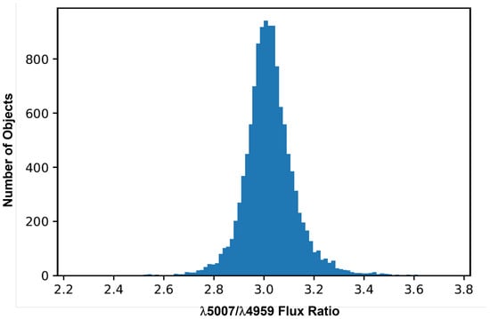
Figure 1.
The 5007/4959 ratio () distribution of all the 12,218 spectra in the first analysis. The distribution is Gaussian, as expected, with a width of 0.133 and a peak at 3.017.

Table 1.
Emission-line properties as a function of z.
2.3. Second Analysis
After concluding this first analysis we noted that the median value of all spectra was 3.017, which is 1.2% higher than the theoretical value of 2.98. To examine why this should be the case, we reran the above analysis with a different software package, MatLab©. We also chose to modify the spectral inclusion criteria to see how a slightly different approach affected the results.
Based on what we learned about the spectral data characteristics from the first analysis, we made the spectral selection parameters for this second analysis more automated. Data were constrained to have a S/N value in the 5007 line > 100, a 5007 line FWHM < 4 Å, and a value between 2 and 4. It is a bit dangerous to reject spectra based on a ratio value when its mean value is the result being calculated. However, as can be seen by Figure 1 the chosen ratio bounds reject only objects that are so far from the mean that their ratio values are clearly corrupt.
After applying these constraints to the data there were 10,817 objects in the remaining data set. These second criteria were more discriminating than the criteria of first analysis, and much easier on our eyes as well. The second data set is essentially a subset of the first.
The data analysis procedure was the same as in the first analysis with one important exception. Rather than fitting the continuum from H through 5007, it was instead fit linearly through the 5007 and 4959 lines separately using continuum values 20 Å on either side of each line. This modified approach was justified by our first rejecting all spectra having 5007 line widths greater than 4 Å so that the continuum through the lines would not be affected by a broad H wing. We found that the median value of in this second analysis was 3.009 ± 0.088. The error significantly improved and the median value lowered but still remained well above the theoretical value. Therefore we conclude that the zeropoint offset found in the first analysis is inherent in the data and/or the general approach to its analysis. In Appendix A, we make the argument that the zeropoint offset is caused by the noise inherent in the data and that a more correct estimate of the median value of is 2.98 ± 0.01.
We list the results of both analyses in Table 1 and plot them in Figure 2 together with horizontal lines marking the mean values of each analysis found by giving each z bin equal weight. The mean values of the two analyses elevate to 3.022 and 3.014, respectively, when weighting each bin equally.
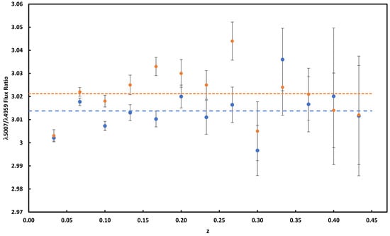
Figure 2.
A plot showing the trend of the 5007/4959 ratio () with redshift as found from the first (orange dots) and second (blue dots) analyses. Data for the plots are given in Table 1. The dashed orange line shows the bin-wise mean value of the first analysis while the dotted blue line shows the same for the second analysis.
2.4. Results
Table 1 presents the median of the value in redshift bins of width 0.033 in z. Column 1 gives the redshift range. The first row is for all objects in the survey, while subsequent rows are broken out by redshift bin. Column 2 lists the number of objects in each bin for the first analysis. Column 3 gives the median of together with its uncertainty, also for the first analysis. The uncertainty is the standard error of the mean found from dividing the standard deviation of each bin by the square root of the number of objects in the bin. Columns 4 and 5 give the same information as in columns 2 and 3 only for the second analysis. These values are plotted in Figure 2.
As shown by Figure 2, the value of shows no obvious trend with increasing redshift to within the error of the data. We found the slope to be quite sensitive to the S/N and line width bounds of each analysis. By allowing the S/N and upper line width bound to vary up and down by 50% from 100 and 4 Å, respectively, we found that the slope of both the first and last analysis varied with a mean value of 0.008 and a 95% confidence interval of ±0.049. Using the 95% confidence interval limits, the variance is between 4.7 and −3.3% out to a z of 0.433.
3. Estimation
Although deriving an estimate of was not a goal at the outset of this work, it was straight-forward to calculate it from our data and we did so following the method of Bahacall et al. [14]. They defined a relation between the wavelengths as
The relationship between this value and is
This leads to the relation of
From a set of 42 AGN, they found an upper limit of corresponding to yr. Applying the same method on a much larger data base of 13,175 quasars from SDSS DR12 yielded corresponding to yr for 0 1.0 [17].
As described in Section 2.2, our fitting procedure calculated the centroid values of each emission line. Using these values for the wavelengths of the 4959,5007 lines, we plot the derived value against z for 0 0.467 in Figure 3. The value for derived from the slope of this line is . This corresponds to yr, which is smaller than the values of [15,16] but larger by a factor of 2.4 than that of [17]. It, together with the previous works, affirms the constancy of with time.
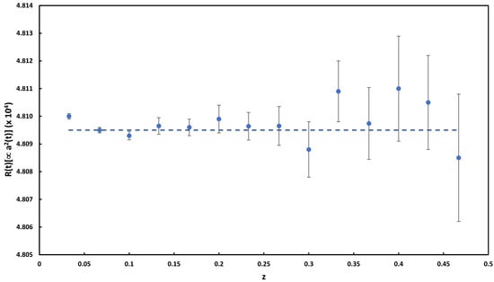
Figure 3.
Data showing the deviation with z. The dashed blue line shows a bests linear fit to the data.
4. Discussion
We have considered emission-line galaxies from the SDSS DR8 which have narrow 4959,5007 lines. We carefully fit these lines with Gaussian profiles and formed a flux ratio, , of their values. We analysed the affect of noise on our derived values. After correcting for noise, we find through two different analytical approaches that the median value of for our data set is 2.98 ± 0.01, in good agreement with previous work.
We find the range of possible variability of to be between 4.7 and −3.3% out to a redshift of z = 0.433. Our results are most consistent with no variability at all. We additionally find no evidence of a change in the fine structure constant greater than yr out to z = 0.467. This is in agreement with previous determinations.
Author Contributions
Conceptualization, J.M.; methodology, M.A.L., C.D.C., D.J. and J.M.; software, M.A.L.; validation, M.A.L., C.D.C. and J.M.; formal analysis, M.A.L., C.D.C., D.J. and J.M.; investigation, M.A.L. and C.D.C.; resources, J.M.; data curation, M.A.L.; writing—original draft preparation, M.A.L. and C.D.C.; writing—review and editing, M.A.L. and J.M.; visualization, M.A.L. and C.D.C.; supervision, J.M.; project administration, J.M.; funding acquisition, J.M. All authors have read and agreed to the published version of the manuscript.
Funding
This research received no external funding.
Institutional Review Board Statement
Not applicable.
Data Availability Statement
The list of SDSS galaxies having emission, galSpecLine-dr8.fits, is available at https://www.sdss.org/dr12/spectro/galaxy_mpajhu/ (accessed on 25 January 2022). The SDSS spectral data referenced by the list are available at https://classic.sdss.org/legacy/index.html (accessed on 25 January 2022).
Acknowledgments
We thank the Brigham Young University Department of Physics and Astronomy for supporting this research. We also thank Jean-François Van Huele for enlightening discussions on atomic processes. Funding for the SDSS and SDSS-II has been provided by the Alfred P. Sloan Foundation, the Participating Institutions, the National Science Foundation, the U.S. Department of Energy, the National Aeronautics and Space Administration, the Japanese Monbukagakusho, the Max Planck Society, and the Higher Education Funding Council for England. The SDSS Web Site is http://www.sdss.org/ (accessed on 25 January 2022). The SDSS is managed by the Astrophysical Research Consortium for the Participating Institutions. The Participating Institutions are the American Museum of Natural History, Astrophysical Institute Potsdam, University of Basel, University of Cambridge, Case Western Reserve University, University of Chicago, Drexel University, Fermilab, the Institute for Advanced Study, the Japan Participation Group, Johns Hopkins University, the Joint Institute for Nuclear Astrophysics, the Kavli Institute for Particle Astrophysics and Cosmology, the Korean Scientist Group, the Chinese Academy of Sciences (LAMOST), Los Alamos National Laboratory, the Max-Planck-Institute for Astronomy (MPIA), the Max-Planck-Institute for Astrophysics (MPA), New Mexico State University, Ohio State University, University of Pittsburgh, University of Portsmouth, Princeton University, the United States Naval Observatory, and the University of Washington.
Conflicts of Interest
The authors declare no conflict of interest.
Abbreviations
The following abbreviations are used in this manuscript:
| The 5007/4959 flux ratio | |
| CMB | Cosmic Microwave Background |
| DR8 | Data Release 8 |
| DR12 | Data Release 12 |
| FWHM | Full Width Half Maximum |
| CDM model | Lambda Cold Dark Matter |
| QSO | Quasi-Stellar Object |
| S/N | Signal to Noise Ratio |
| SDSS | Sloan Digital Sky Survey |
Appendix A. Noise Bias Analysis
As it turns out, the relatively high mean values of are from noise injecting a systematic bias into the fitted line flux values. To examine as a function of S/N, we generated a series of 4959 and 5007 Gaussian line profiles having varying degrees of noise, then fitted them with our software routines.
We constructed the model spectra by first choosing a continuum base value randomly between 5 and 100. A slope having a mean of −0.0005 and a standard deviation of 0.005 was then applied to it. These parameters are based on the range found in the SDSS data. Next the 4959 and 5007 lines were generated from Gaussian profiles and added to the continua. The amplitude of the 4959 line was fixed at 200 while the amplitude of the 5007 was set a factor of 2.985 higher. We constrained the widths of the lines be the same within each spectrum but allowed them to vary randomly from spectrum to spectrum within a FWHM range of 3 to 10 Å. In all, 1000 spectra were generated.
We then created eight new spectra from each individual spectrum by adding different levels of Gaussian random noise such as to make the S/N value of the integrated 5007 line flux equal to 100, 45, 30, 18, 13, 9, 7, and 6. We then placed each of these eight noise-modified spectra through the Gaussian fitting routines described in Section 2.1 and Section 2.2. An interesting pattern emerged which is shown by the plots in Figure A1. At all noise levels, even when no noise was added, there was a tail in the distribution of values toward higher numbers. As the noise level increases, this tail also increases in number and length. This is likely because in forming a ratio, the spread from error on the lower value side of the distribution can only extend towards the value of zero but no further. However the spread on the opposing side can extend indefinitely, having no numerical limit. As a result there is a natural statistical bias toward higher ratio values in higher noise levels.
There is a second, even greater effect. As noise increases, the peak of the distribution shifts toward smaller values. Apparently, the fitting routines have a penchant for overestimating line flux as noise increases. Since the 4959 line always has a lower S/N, the values will be driven to lower numerical values as noise increases. These two effects are shown in Figure A1. The overall trend with noise is given in Figure A2.
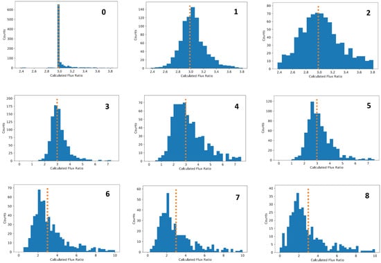
Figure A1.
Histogram plots of the frequency of values (labeled “Calculated Flux Ratio”) for inreasing noise levels. The numeral in the upper right corner of each plot corresponds to the S/N ratio of the flux in the 5007 line as follows: 0 = no added noise, 1 = 100, 2 = 45, 3 = 30, 4 = 18, 5 = 13, 6 = 9, 7 = 7, and 8 = 6. For all values, including no added noise, there is a higher-value tail in the distribution. As S/N decreases, the peak shifts increasingly to the left.
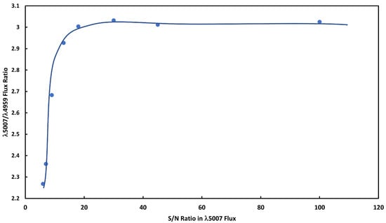
Figure A2.
The median value for found from the data presented in Figure A1. Low S/N values drive the median values of lower until the S/N of the 5007 line is 18. For S/N values above this, the values increases and peaks at approximately 3.20 at a S/N of 13. As S/N increases above this, the median values ramp linearly toward the nominal value in the modeled data of 2.985 for no noise.
The value of for 5007 S/N values of 100 in our model spectra is 3.02. This trends toward lower values as S/N increases. The median 5007 S/N of objects in our second sample is 134. An estimate of our calculated value for a S/N of 134 is 3.015 ± 0.005. Therefore noise adds an offset of 0.030 to our median values. With this adjustment, the median value of the first analysis changes from 3.017 to 2.987. For the second analysis it changes from 3.009 to 2.979. Averaging these two values and taking the precision of the estimate to be two significant digits, we obtain a value for of 2.98 ± 0.01.
Appendix B. Examples of Spectra
This appendix contains examples of spectra that met criteria for inclusion or rejection in the first analysis.
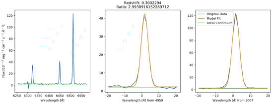
Figure A3.
Typical data for a fit that was deemed acceptable.
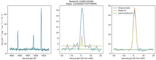
Figure A4.
A rejected spectrum where the Gaussian fit (orange line) clearly did not match the shape of the 4959 emission line.
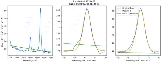
Figure A5.
A spectrum where the continuum fit (green line) clearly cuts off the bottom of the 4959 emission line.
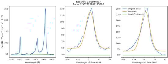
Figure A6.
A spectrum where the continuum fit (green line) falls below the bottom of both unusually broadened emission lines.
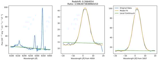
Figure A7.
A spectrum with a broad H line that artificially elevated the placement of the continuum level (green line).
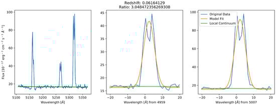
Figure A8.
A spectrum having two noticeable peaks per emission line as is common for galaxy mergers [27].
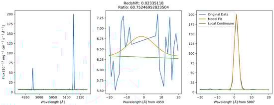
Figure A9.
A spectrum where the 4959 line was mistakenly subtracted out of the spectrum in the data-reduction pipeline. Such instances were rare.
References
- Galavís, M.E.; Mendoza, C.; Zeippen, C.J. Atomic data from the IRON Project*—XXII. Radiative rates for forbidden transitions within the ground configuration of ions in the carbon and oxygen isoelectronic sequences. Astronony Astrophys. Suppl. Ser. 1997, 123, 159–171. [Google Scholar] [CrossRef] [Green Version]
- Dimitrijević, M.S.; Popović, L.Č.; Kovačević, J.; Dačić, M.; Ilić, D. The flux ratio of the [OIII]λλ5007,4959 lines in AGN: Comparison with theoretical calculations. Mon. Not. R. Astron. Soc. 2007, 374, 1181–1184. [Google Scholar] [CrossRef] [Green Version]
- Osterbrock, D.E.; Ferland, G.J. Astrophysics of Gaseous Nebulae and Active Galactic Nuclei; University Science Books: Melville, NY, USA, 2006. [Google Scholar]
- Storey, P.J.; Zeippen, C.J. Theoretical values for the [OIII] 5007/4959 line-intensity ratio and homologous cases. Mon. Not. R. Astron. Soc. 2000, 312, 813–816. [Google Scholar] [CrossRef]
- Uzan, J.P. Varying Constants, Gravitation and Cosmology. Living Rev. Relativ. 2011, 14, 2. [Google Scholar] [CrossRef] [Green Version]
- Webb, J.K.; Flambaum, V.V.; Churchill, C.W.; Drinkwater, M.J.; Barrow, J.D. Search for Time Variation of the Fine Structure Constant. Phys. Rev. Lett. 1999, 82, 884–887. [Google Scholar] [CrossRef] [Green Version]
- Webb, J.K.; Murphy, M.T.; Flambaum, V.V.; Dzuba, V.A.; Barrow, J.D.; Churchill, C.W.; Prochaska, J.X.; Wolfe, A.M. Further Evidence for Cosmological Evolution of the Fine Structure Constant. Phys. Rev. Lett. 2001, 87, 091301. [Google Scholar] [CrossRef] [Green Version]
- Chand, H.; Srianand, R.; Petitjean, P.; Aracil, B.; Quast, R.; Reimers, D. Variation of the fine-structure constant: Very high resolution spectrum of QSO HE 0515-4414. Astron. Astrophys. 2006, 451, 45–56. [Google Scholar] [CrossRef] [Green Version]
- Fritzsch, H.; Solà, J.; Nunes, R.C. Running vacuum in the Universe and the time variation of the fundamental constants of Nature. Eur. Phys. J. C 2017, 77, 1–16. [Google Scholar] [CrossRef]
- Leszczńska, K.; Balcerzak, A.; Dąbrowski, M.P. Varying constants quantum cosmology. J. Cosmol. Astropart. Phys. 2015, 2015, 012. [Google Scholar] [CrossRef] [Green Version]
- Balcerzak, A.; Dąbrowski, M.P.; Salzano, V. Modelling Spatial Variations of the Speed of Light. Annalen der Physik 2017, 529, 1600409. [Google Scholar] [CrossRef] [Green Version]
- Dąbrowski, M. Singularities and Cyclic Universes. Acta Phys. Pol. B Proc. Suppl. 2017, 10, 415. [Google Scholar] [CrossRef] [Green Version]
- Petrov, Y.V.; Nazarov, A.I.; Onegin, M.S.; Petrov, V.Y.; Sakhnovsky, E.G. Natural nuclear reactor at Oklo and variation of fundamental constants: Computation of neutronics of a fresh core. Phys. Rev. C 2006, 74, 064610. [Google Scholar] [CrossRef] [Green Version]
- Bahcall, J.N.; Steinhardt, C.L.; Schlegel, D. Does the Fine-Structure Constant Vary with Cosmological Epoch? Astrophys. J. 2004, 600, 520–543. [Google Scholar] [CrossRef] [Green Version]
- Gutiérrez, C.M.; López-Corredoira, M. The Value of the Fine Structure Constant over Cosmological Times. Astrophys. J. 2010, 713, 46–51. [Google Scholar] [CrossRef] [Green Version]
- Rahmani, H.; Maheshwari, N.; Srianand, R. Constraining the variation in the fine-structure constant using SDSS DR7 quasi-stellar object spectra. Mon. Not. R. Astron. Soc. 2014, 439, L70–L74. [Google Scholar] [CrossRef]
- Albareti, F.D.; Comparat, J.; Gutiérrez, C.M.; Prada, F.; Pâris, I.; Schlegel, D.; López-Corredoira, M.; Schneider, D.P.; Manchado, A.; García-Hernández, D.A.; et al. Constraint on the time variation of the fine-structure constant with the SDSS-III/BOSS DR12 quasar sample. Mon. Not. R. Astron. Soc. 2015, 452, 4153–4168. [Google Scholar] [CrossRef] [Green Version]
- Zhang, J.J.; Yin, L.; Geng, C.Q. Cosmological constraints on Λ(α)CDM models with time-varying fine structure constant. Ann. Phys. 2018, 397, 400–409. [Google Scholar] [CrossRef] [Green Version]
- Marsh, M.C.D. Exacerbating the Cosmological Constant Problem with Interacting Dark Energy Models. Phys. Rev. Lett. 2017, 118, 011302. [Google Scholar] [CrossRef] [Green Version]
- Kotuš, S.M.; Murphy, M.T.; Carswell, R.F. High-precision limit on variation in the fine-structure constant from a single quasar absorption system. Mon. Not. R. Astron. Soc. 2017, 464, 3679–3703. [Google Scholar] [CrossRef]
- Colaço, L.R.; Holanda, R.F.L.; Silva, R. Probing variation of the fine-structure constant using the strong gravitational lensing. arXiv 2020, arXiv:2004.08484. [Google Scholar]
- Lopez-Honorez, L.; Mena, O.; Palomares-Ruiz, S.; Villanueva-Domingo, P.; Witte, S.J. Variations in fundamental constants at the cosmic dawn. J. Cosmol. Astropart. Phys. 2020, 2020, 026. [Google Scholar] [CrossRef]
- Landau, S.J. Variation of fundamental constants and white dwarfs. arXiv 2020, arXiv:2002.00095. [Google Scholar] [CrossRef]
- Gonçalves, R.S.; Landau, S.; Alcaniz, J.S.; Holanda, R.F.L. Variation in the fine-structure constant and the distance-duality relation. J. Cosmol. Astropart. Phys. 2020, 2020, 036. [Google Scholar] [CrossRef]
- Stoughton, C.; Lupton, R.H.; Bernardi, M.; Blanton, M.R.; Burles, S.; Castander, F.J.; Connolly, A.J.; Eisenstein, D.J.; Frieman, J.A.; Hennessy, G.S.; et al. Sloan Digital Sky Survey: Early Data Release. Astron. J. 2002, 123, 485–548. [Google Scholar] [CrossRef]
- Chen, Y.M.; Kauffmann, G.; Tremonti, C.A.; White, S.; Heckman, T.M.; Kovač, K.; Bundy, K.; Chisholm, J.; Maraston, C.; Schneider, D.P.; et al. Evolution of the most massive galaxies to z = 0.6 − I. A new method for physical parameter estimation. Mon. Not. R. Astron. Soc. 2012, 421, 314–332. [Google Scholar] [CrossRef]
- Maschmann, D.; Melchior, A.L.; Mamon, G.A.; Chilingarian, I.V.; Katkov, I.Y. Double-peak emission line galaxies in the SDSS catalogue. Astron. Astrophys. 2020, 641, A171. [Google Scholar] [CrossRef]
Publisher’s Note: MDPI stays neutral with regard to jurisdictional claims in published maps and institutional affiliations. |
© 2022 by the authors. Licensee MDPI, Basel, Switzerland. This article is an open access article distributed under the terms and conditions of the Creative Commons Attribution (CC BY) license (https://creativecommons.org/licenses/by/4.0/).