Article

Coaxiality Optimization Analysis of Plastic Injection Molded Barrel of Bilateral Telecentric Lens

Department of Mechanical and Energy Engineering, National Chiayi University, Chiayi 600355, Taiwan
*
Author to whom correspondence should be addressed.
Symmetry 2022, 14(2), 200; https://doi.org/10.3390/sym14020200
Submission received: 18 December 2021 / Revised: 17 January 2022 / Accepted: 18 January 2022 / Published: 20 January 2022
(This article belongs to the Special Issue Axisymmetry in Mechanical Engineering)

Abstract

:
Plastic optical components are light in weight, easy to manufacture, and amenable to mass production. However, plastic injection molded parts are liable to shrinkage and warpage as a result of the pressure and temperature variations induced during the molding process. Consequently, controlling the process parameters in such a way as to minimize the geometric deformation of the molded part and improve the performance of the optical component as a result remains an important concern. The present study considered the problem of optimizing the injection molding parameters for the plastic lens barrel of a bilateral telecentric lens (BTL) containing four lens assemblies. The study commenced by using CODE V optical software to design the lens assemblies and determine their optimal positions within the barrel. Taguchi experiments based on Moldex3D simulations were then performed to determine the processing conditions (i.e., maximum injection pressure, maximum packing pressure, melt temperature, mold temperature, and cooling time) which minimize the coaxiality of the plastic barrel. Finally, CODE V and grayscale analyses were performed to confirm the optical performance of the optimized BTL. The Taguchi results show that the coaxiality of the plastic lens barrel is determined mainly by the maximum packing pressure and melt temperature. In addition, the CODE V and grayscale analysis results confirm that the optimized BTL yields a better modulus transfer function, spot diagram performance, and image quality than a BTL produced using the general injection molding parameters.

1. Introduction

Plastic provides an ideal material for the fabrication of optoelectronic product accessories and supports due to its light weight, low cost, high mechanical strength, ease of processing, and good potential for mass production. However, the successful realization of plastic optical components involves many challenges, including optical design, integrated mechanism design, process parameter design, and product inspection and analysis. Plastic optical products are commonly fabricated using injection molding. However, while injection molding has significant advantages in terms of a high throughput, a low unit cost, and good repeatability, the quality of the molded components is extremely sensitive to the processing conditions, e.g., the injection pressure, packing pressure, melt temperature, mold temperature, packing time, and cooling time. Moreover, the processing parameters have both individual and interactive effects on the molding outcome. Consequently, determining the processing conditions which optimize the quality of the molded products (the dimensional tolerance, surface finish, mechanical strength, etc.) is extremely complex.
Optical components are subject to extremely tight manufacturing tolerances in order to achieve the necessary imaging quality. However, achieving these tolerances for plastic components realized through injection molding is extremely challenging, particularly in the case of geometric assemblies with high aspect ratios, or non-symmetrical geometries [1,2,3,4]. In many lens-based devices, the lens assemblies are housed within plastic bodies, and hence the problem of ensuring the imaging quality of the device involves not only guaranteeing the optical quality of the individual lenses, but also controlling the geometrical precision and form of the housing. For example, for bilateral telecentric lenses (BTLs), which are designed to provide a constant field of view (FOV) at all distances from the lens, roundness or concentricity errors of the lens barrel result in misalignments of the lens assemblies, which then seriously degrade the performance of the device. As a result, it is essential that the molding parameters are correctly controlled in such a way as to minimize the shrinkage, warpage, and residual stress of the barrel during the manufacturing process [5,6,7].
Many studies have demonstrated the feasibility of combining the Taguchi experimental method with mold flow simulations to determine the optimal injection molding processing parameters through a minimum number of experiential trials [8,9,10,11]. Furthermore, many software systems and algorithms have been applied to evaluate existing optical designs, optimize the performance of new imaging solutions, reduce manufacturing costs through process improvements, etc. [12,13,14,15,16,17]. Among the many optical design software packages currently available, CODE V (Synopsys, Inc., Mountain View, California, USA) is one of the most commonly used for the design, tolerancing, and performance evaluation of new optical configurations.
In the present study, a hybrid Taguchi/Moldex3D simulation approach was employed to optimize the injection molding processing parameters for the plastic lens barrel of the BTL device shown in Figure 1 consisting of four lenses and a protruding handle. Optimal analysis of plastic injection molding was based on the authors’ previous research on the roundness and concentricity of the BTL [18]. The authors performed further optical analysis on the concentricity results to confirm the optimized results. CODE V optical software was first used to design the four lenses and to determine their optimal positions within the barrel. Taguchi/Moldex3D simulations were then performed to establish the injection molding conditions which minimize the coaxiality error of the lens barrel (i.e., the overall concentricity error of the four lenses) following the molding process. Finally, CODE V and grayscale analyses were performed to investigate the modulus transfer function (MTF), spot diagram characteristics, and imaging performance of the optimized BTL barrel.

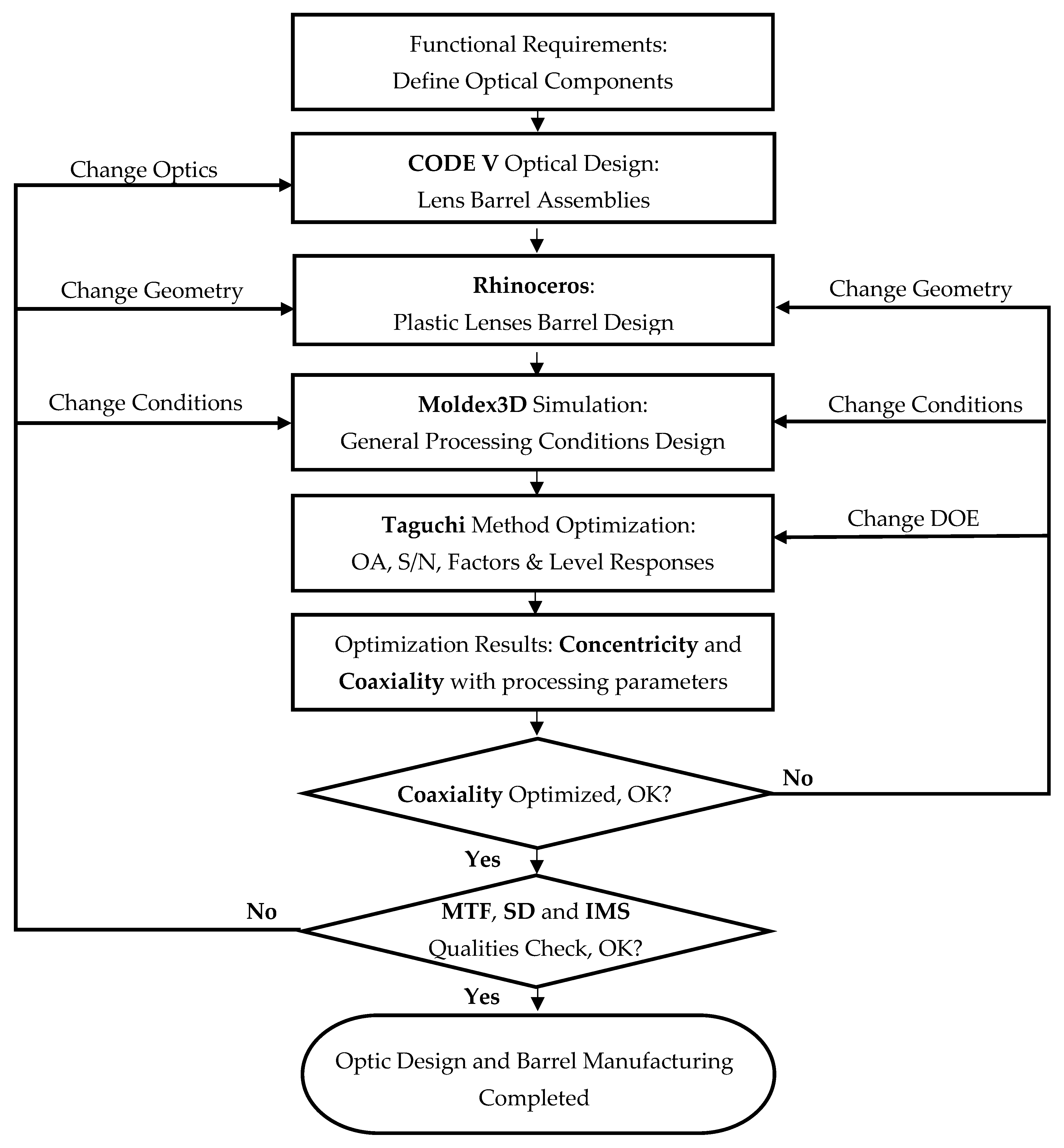
2. Method and Procedures

Figure 2 presents a flow chart showing the main steps in the design, optimization, and analysis procedure performed in the present study. Having defined the optical components within the BTL (i.e., the four lenses), CODE V optical software was employed to establish the specification, location, and material of each lens and to determine the required geometrical dimensions of the optical tube. A model of the plastic optical tube was constructed using Rhinoceros software, and Moldex3D simulations were then performed in conjunction with the Taguchi experimental design method to determine the optimal injection molding conditions which minimize the average concentricity error of the optical tube at the planes corresponding to the ideal locations of the four lenses. Finally, the MTF and spot diagram of the BTL were investigated for three different light fields (FI, FII, and FIII) entering the objective lens at different distances from the optical axis (see Figure 1). The validity of the optimized design was confirmed by comparing the CODE V results for the modulus transfer function (MTF), spot diagram (SD), and 2D imaging simulation (IMS) of the proposed optical device with those of an ideal BTL device with no coaxiality or concentricity errors and a BLT device molded using the default processing conditions for the selected polymer material.

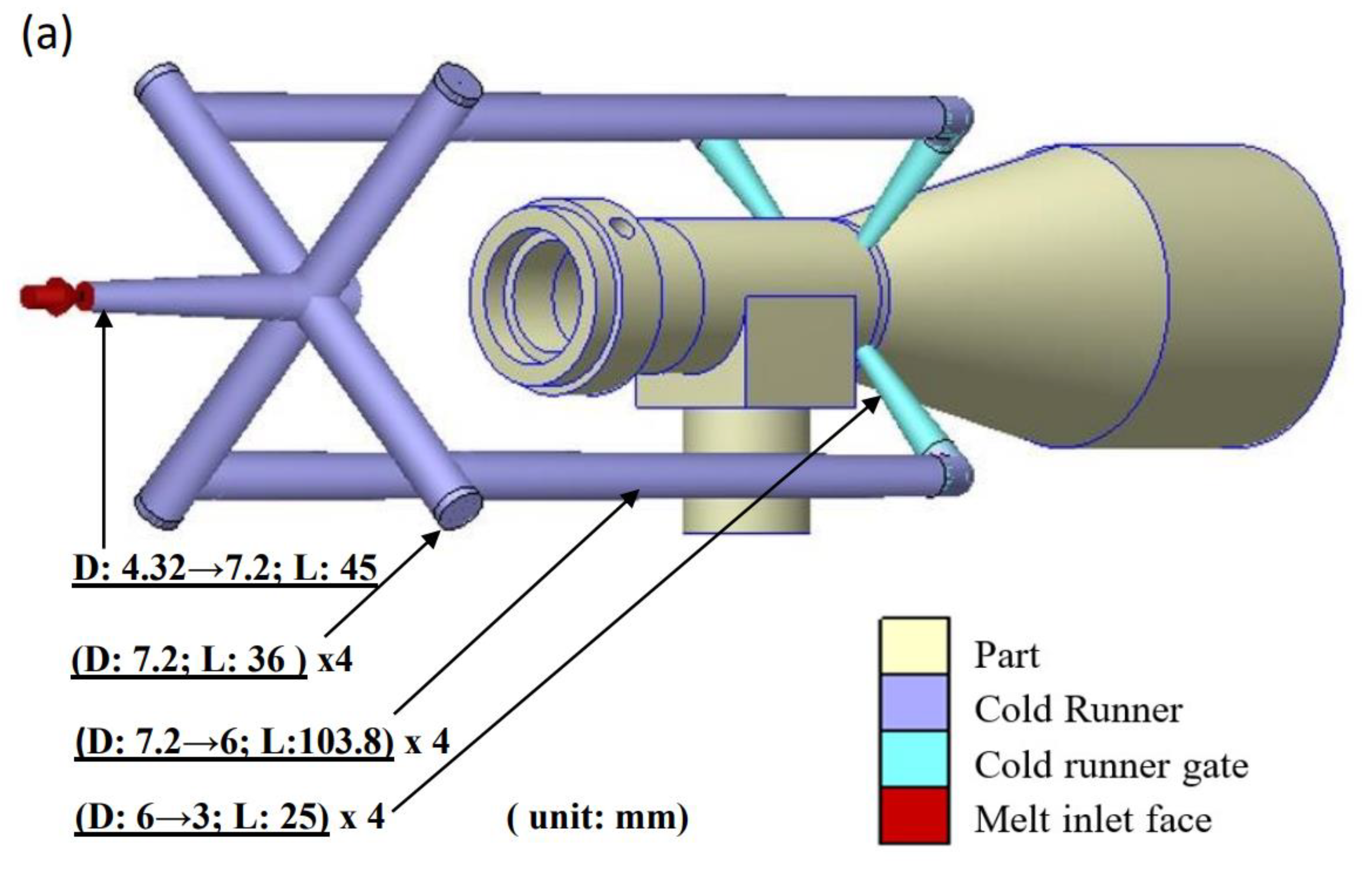
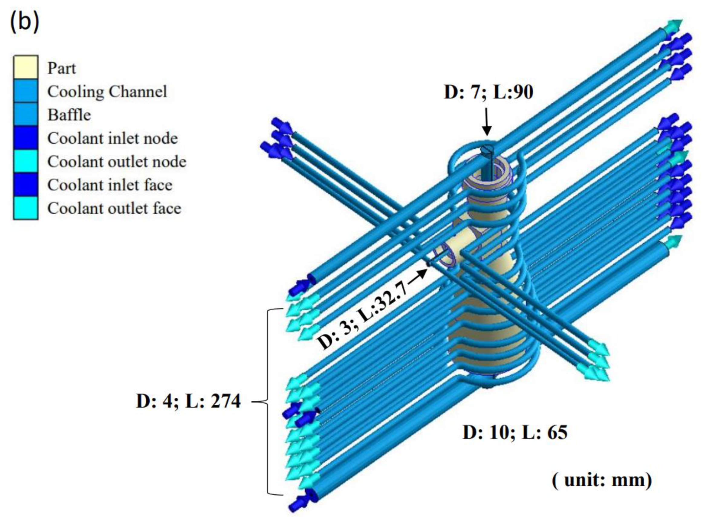
2.1. Materials and Geometry Model

In performing the analysis, it was assumed that the plastic barrel of the BTL was fabricated of PA66 (Polyamide 66 or Nylon 66) polymer (TECHNYL A 216, Solvay Engineering Plastics), with the material properties and recommended injection molding parameters shown in Table 1. Figure 3a shows the relationship between the viscosity of PA66 and the shear rate at different temperatures. Figure 3b shows the P-v-T (pressure/specific volume/temperature) properties of the PA66 material as a function of the shear rate and temperature, and this characteristic was used to calculate the degree of compression of the PA66 material in the packing stage. Table 2 shows the material, geometry dimensions, and optical properties of the four lenses within the BTL.

2.2. Mold Flow Analysis and Taguchi Experimental Method

A geometric model of the BTL barrel was constructed in Rhinoceros and exported to Moldex3D-Mesh to define the corresponding molding system (see Figure 4) with the runner system (see Figure 4a) and cooling system (see Figure 4b). Figure 4a shows that the PA66 melt was injected into the mold cavity with four gates through the runner system, and the size of the runners including the diameter and length is shown in the description. The coolant used in the entire injection molding system was water, and the water entered the cooling runner at a temperature of 25 °C to cool the mold (see Figure 4b). The injection molding process was then simulated using Moldex3D. The simulations considered five molding parameters, namely, the maximum injection pressure, the maximum packing pressure, the melt temperature, the mold temperature, and the cooling time. Each molding parameter (control factor) was assigned four different level settings. Hence, the Taguchi experiments were configured in an L16(54) orthogonal array (OA), as shown in Table 3 (gray region). The aim of the Taguchi experiments (i.e., Moldex3D simulations) was to determine the combination of control factor level settings which minimized the concentricity error of the BTL barrel at the position of each lens and hence optimized the coaxiality of the tube. Hence, for each run of the OA, the quality of the simulation outcome was evaluated using the following smaller-the-better S/N (signal-to-noise) ratio:
S / N = 10 log ( 1 n i = 1 n y i 2 )   ,  
where y i is the concentricity of the barrel at the measurement plane i (i = 1~4), and n is the number of measured points in the trial.

2.3. Roundness, Concentricity, and Coaxiality Measures

For cylindrical objects such as the BTL barrel considered in the present study, the manufacturing quality can be evaluated by three different metrics: the roundness, the concentricity, and the coaxiality. Traditional methods for evaluating the roundness of manufactured parts include the least squares circle (LSC) method, the minimum zone tolerance circle (MZC) method, the maximum inscribed circle (MIC) method, and the minimum circumscribed circle (MCC) method [19]. In the present study, the roundness of the BTL barrels produced using the different processing conditions specified in the Taguchi OA was evaluated using the LSC method [20]. In particular, a fitting process was applied to determine the circle which produced the minimum sum of the square error F(x, y) with the actual circular profile of the tube, i.e.,
F ( x , y ) = i = 1 n [ r ( x , y ) 2 R c 2 ] 2 = i = 1 n [ ( x x c ) 2 + ( y y c ) 2 R c 2 ] 2
where r(x, y) is the distance between the measured point (x, y) and the unknown center (xc, yc) of the circle, n is the number of measured points, and Rc is the radius of the least squares circle. Taking the center (xc, yc) of the least squares error (LSE) circle as the center of the circle after processing deformation, the LSE circle center was calculated at each of the four reference planes (i.e., lens positions) in the BTL barrel. The concentricity, d, of the barrel at each plane was then computed as the offset of the LSE circle center from the designed datum value (xo, yo) = (0, 0). Finally, the concentricity values obtained at the four reference planes were averaged to evaluate the coaxiality of the tube [21,22,23]. For convenience, the corresponding mathematical derivations are given in the following.
The concentricity of the BTL at plane i was evaluated as
d i = ( x c x o ) 2 + ( y c y o ) 2
The coaxiality (overall concentricity) of the BTL was computed as
Coaxiality = i = 1 n [ d i ] 2 / n

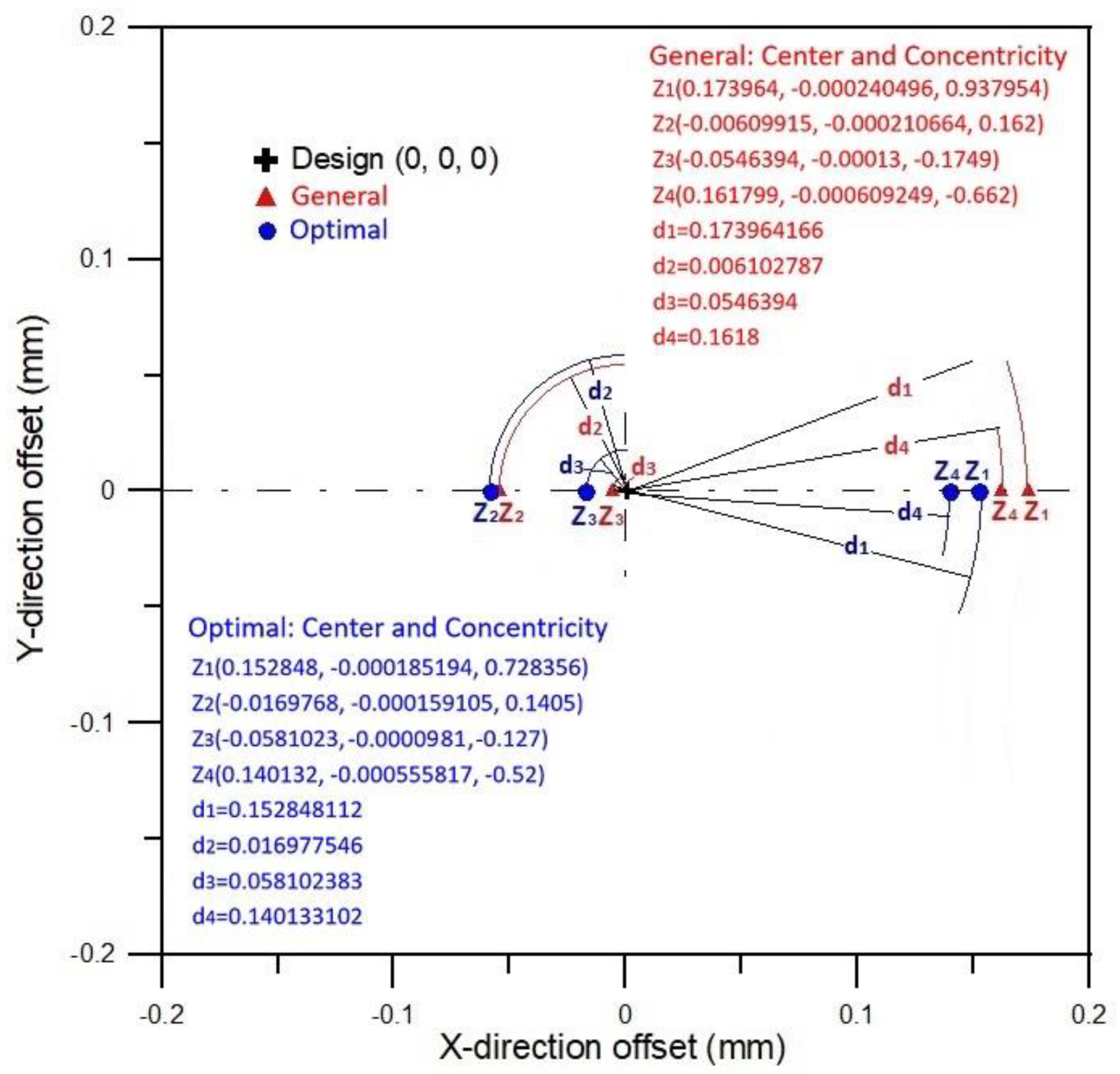
2.4. CODE V Optical Evaluation Using Eccentric Coordinates (xc, yc, zc)

Following the Taguchi/Moldex3D simulations, the concentricity coordinates (xc, yc) and axial displacements (zc) of each lens in the barrel were input to CODE V software in order to evaluate the optical performance of the device. The performance was evaluated in terms of three metrics, namely, the MTF, the spot diagram, and the 2D imaging simulation. In general, the MTF indicates how a lens reproduces contrast over a broad range of spatial frequencies, while the spot diagram computes the focused image size and provides a quick and qualitative assessment of the overall quality of the lens assembly. Finally, the 2D imaging simulation (resolution results with grayscale analysis) provides a further simple visualization of the optical system performance [24].

3. Results and Discussion

3.1. Taguchi Optimization Results

The general (or standard for specific machines) processing parameters for the considered PA66 polymer material were taken from the manufacturer’s specification as follows: maximum injection pressure 200 MPa, maximum packing pressure 200 MPa, melt temperature 280 °C, mold temperature 80 °C, and cooling time 13 s (see the upper row in Table 3). However, the Taguchi analysis results indicated that the optimal parameter settings (i.e., the parameter settings which minimized the coaxiality error of the BTL tube) were a maximum injection pressure of 220 MPa, a maximum packing pressure of 240 MPa, a melt temperature of 275 °C, a mold temperature of 90 °C, and a cooling time of 17 s (see the lower row in Table 3). Table 4 shows the Taguchi S/N response data for the five control factors and their level settings. As shown, the control factors can be ranked in terms of a diminishing effect on the coaxiality of the tube as follows: maximum packing pressure > melt temperature > cooling time > maximum injection pressure > mold temperature. In other words, the coaxiality of the molded tube is dominated by the packing pressure and melt temperature, while the cooling time, injection pressure, and mold temperature all have more minor effects. Table 4 shows that the S/N ranges of factor A (maximum injection pressure) and factor D (molding temperature) are much smaller than those of factor B (maximum packing pressure), factor C (melt temperature), and factor E (cooling time). It is worth noting that under the condition of coaxial optimization of control factors A and D, their individual influence is significantly smaller than that of other factors (B, C, and E). However, factor A and factor D are different in the S/N range (but their values are very close). Therefore, their impact evaluation should be discussed in consideration of other different processing conditions.
In general, the results show that a larger maximum packing pressure, a lower melt temperature, and a longer cooling time are beneficial in reducing the concentricity error (in each plane) of the tube and improving the coaxiality as a result. Table 5 shows the injection molding simulation parameters for the general design and the optimal design to verify the results of the Taguchi method.
Figure 5 shows the real sprue pressure changes and real flow rate changes in the filling stage and the packing stage after the injection molding simulation. It can be seen that increasing the maximum packing pressure and the maximum injection pressure helps to maintain the stability of the flow rate (about 31.97 cm3/s) and is very close to the expected constant flow rate (34.05 cm3/s). For the V/P (velocity-to-pressure) transition point, the general design and optimal design have values of 2.098 s and 2.097 s, respectively. The setting of the maximum injection pressure helps to keep the flow rate at a certain level during the filling stage and limits the injection pressure during the filling stage to prevent mold or machine failure. In fact, the real injection pressure also changes at the set desired flow rate, and the real injection pressure is always less than the maximum injection pressure during the filling stage. On the other hand, an injection molding machine with such a high maximum packing pressure setting (200 MPa) is an extreme upper limit and is not widely used throughout the process. Because this paper is a numerical simulation analysis, the setting of the packing pressure does not fully consider the actual situation. Generally speaking, when the packing pressure is too high, the pressure in the mold will be too large. Such a processing procedure can cause stress concentration and residual stress, which can lead to difficulty in ejection and even cracking. For the peak flow rate shown in Figure 5, this is not a typical velocity profile for injection molding. The possible reason is that the numerical simulation in this study adopted a one-stage flow rate setting. Under the influence of all the complex processing factors, the cavity space that is not fully filled must be filled before the expected end of time. Therefore, there is a tendency for the flow rate to suddenly increase before entering the packing stage. Of course, this situation still needs further confirmation and discussion.
Figure 6 plots the coaxiality error and S/N values for each of the 16 runs in the L16(54) OA, together with those for the general (i.e., recommended) processing parameters and optimal processing parameters. As shown, the tube produced using the optimal molding parameters has the maximum S/N value of 19.33078 dB and the minimum coaxiality error of 0.011666 mm2. The S/N value and coaxiality error of the optimal tube are 5.76% higher and 21.5% lower, respectively, than those of the tube produced using the recommended processing parameters. In other words, the effectiveness of the optimized parameter settings in improving the coaxiality of the BTL tube is confirmed.

3.2. Geometry Analysis

Table 6 and Figure 7 show the center coordinate positions and concentricity values at the four reference planes (Z1~Z4) of the ideal BTL design (with zero concentricity and coaxiality errors), and the BTL tubes produced using the general and optimal processing conditions. The results indicate that the geometric distortion produced by the manufacturing process is far less than that produced by the asymmetric design of the barrel itself (i.e., the protruding handle structure (see Figure 1)). In addition, the optimal process parameters have a greater effect in reducing the concentricity error at measurement planes Z1 and Z4 (at the two ends of the BTL barrel) than at planes Z2 and Z3 (in the central region of the barrel). Notably, however, the results presented in Figure 7 show that even though the concentricity values at the four planes are not markedly improved in the optimal design, the overall coaxiality of the tube is significantly improved compared to that of the tube produced using the general parameters (i.e., from 0.014866 to 0.011666 mm, as shown in Table 6). It should be noted that the runner design and cooling system in this study are based on virtual simulation. If the injection molding process is to be carried out realistically, the interference problem caused by the mold assembly must be considered.

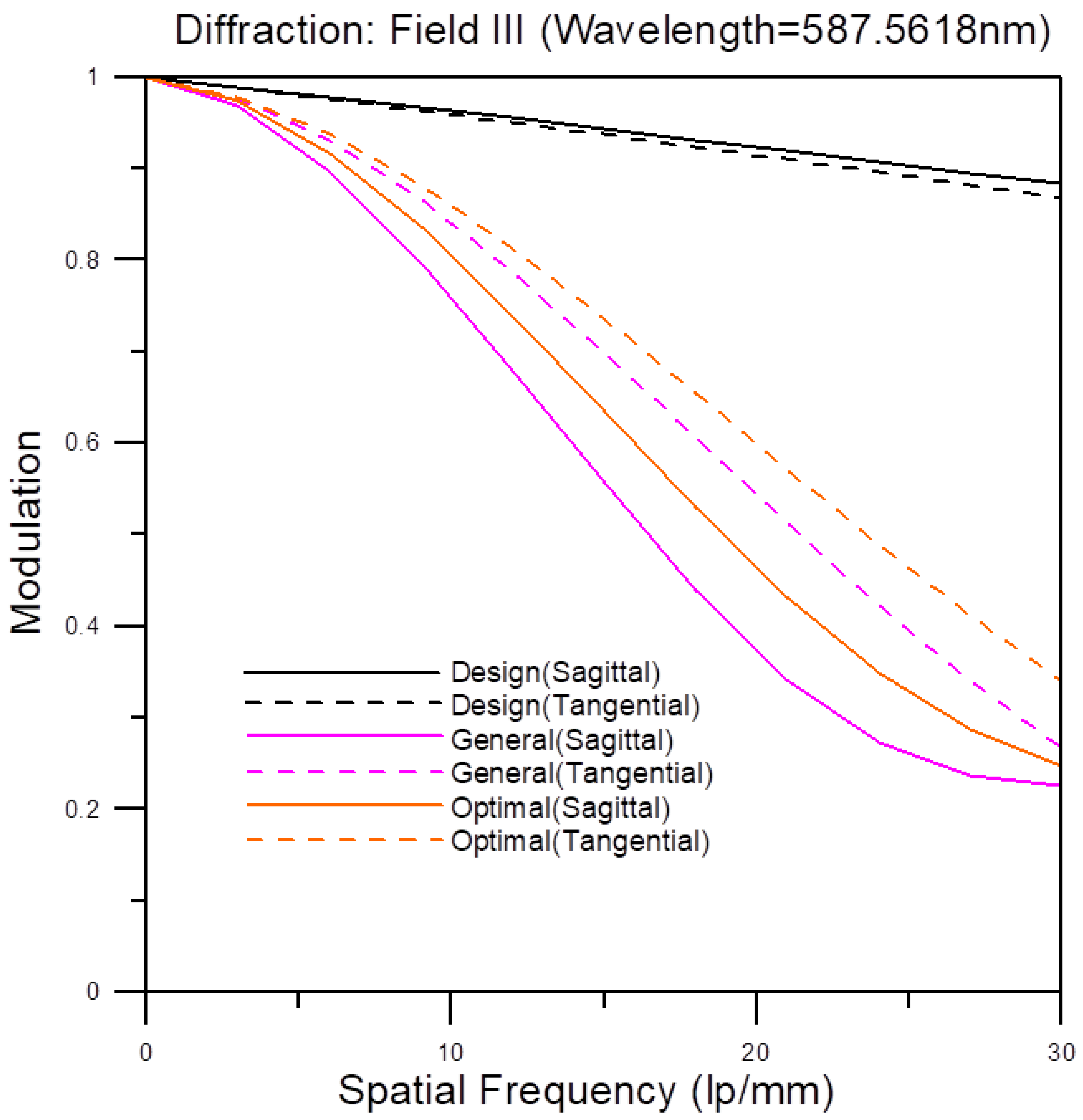
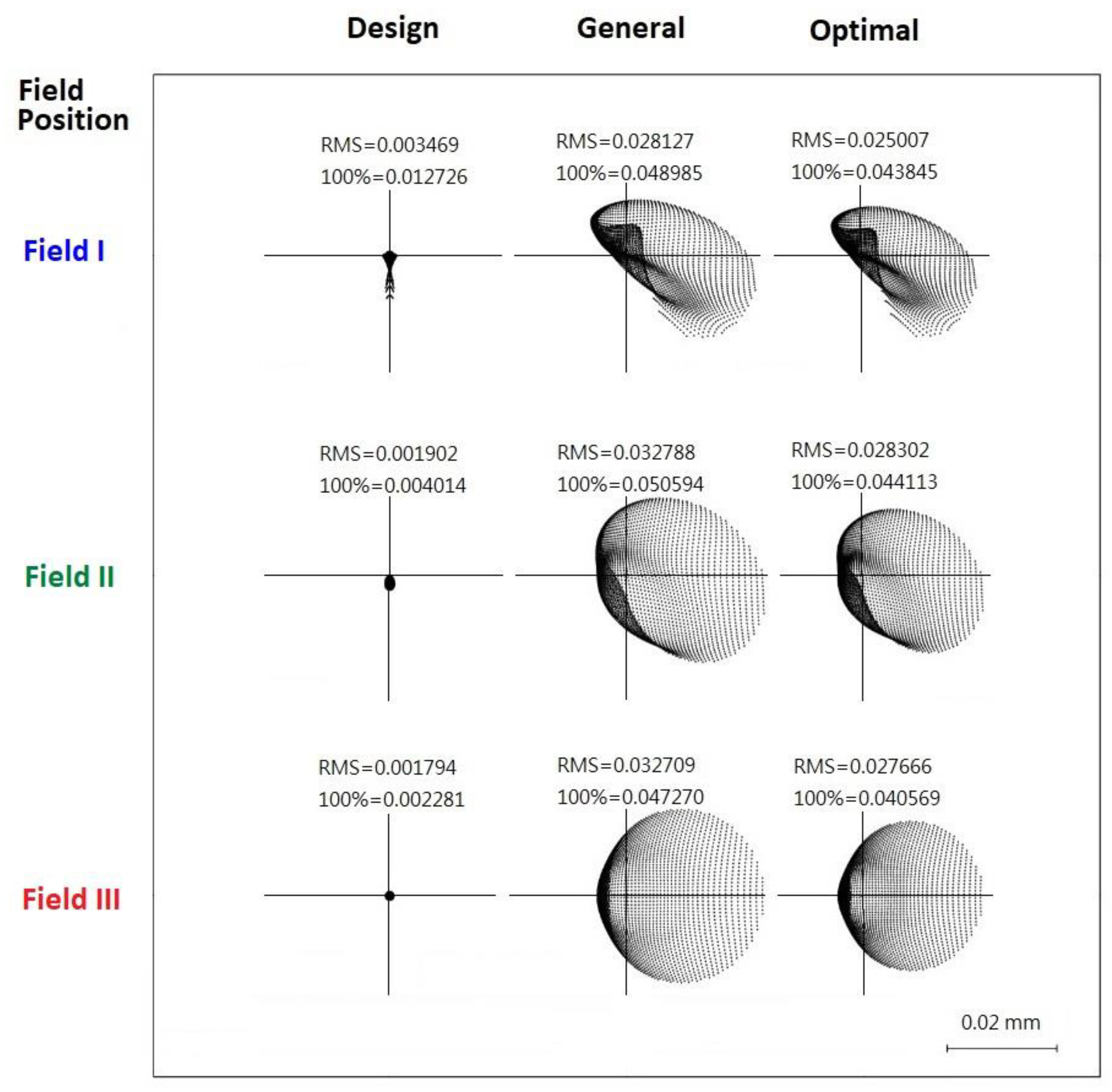
3.3. Optical Performance

As described in Section 2.4, the optical performance of the BTL barrel produced using the optimal processing conditions was evaluated by means of MTF plots, spot diagrams, and 2D imaging simulations. For comparison purposes, CODE V simulations were also performed for the ideal design barrel and for the BTL barrel produced using the general processing conditions. Note that the center coordinates and concentricity values of the four lenses in each barrel were assigned the values shown in Table 6.
Figure 8 shows the sagittal and tangential MTF curves of the three BTL tubes (designated as design, general, and optimal) for light fields FI, FII, and FIII (see Figure 1). In general, an MTF curve closer to the diffraction limit curve indicates a better imaging performance. Consequently, all six MTF curves for the ideal BTL design (with zero concentricity errors) are virtually superimposed on the diffraction limit curve. Moreover, the MTF curves for the optimal tube are closer to the diffraction limit curve than those of the general tube. In other words, the optimized parameters yield a significant improvement in the optical performance of the BTL tube compared to that of the tube produced using the general processing parameters. Figure 9, Figure 10 and Figure 11 provide a detailed analysis of the imaging performance of the three tubes for light fields I, II, and III. In general, the results confirm that, for all three light fields, the imaging performance of the optimal tube is closer to the ideal performance than that of the general tube. Furthermore, comparing the three figures, it is seen that the imaging performance of the general tube and optimal tube is close to that of the ideal tube for light rays close to the optical axis of the BTL (i.e., FIII) but gradually degrades with an increasing distance from the axis (i.e., FII and FI).
Figure 12 shows the spot diagrams of the three light fields on the image plane of the design, general, and optimal BTL tubes. Note that for each spot, the RMS (root mean square) value indicates the root mean square values of all the light spot distribution coordinates, while the 100% value indicates the smallest circle diameter (in mm) sufficient to encompass all of the individual light spots within the light field. Observing the three sets of light spots for each tube, it is clear that the optimal tube results in a sharper imaging performance than the general tube. Furthermore, examining the spot diagrams for light field FIII (closest to the optical axis), the minimum circumscribed circle diameters of the design, general, and optimal tubes are found to be 0.002281 mm, 0.047270 mm, and 0.040569 mm, respectively. In other words, the optimal tube reduces the focused spot size by 14.2% compared to that of the general tube. The corresponding improvement values for the FII and FIII fields are 12.8% and 10.5%, respectively. Similarly, the optimal tube improves the RMS value of the focus spot size by 15.4% compared to that of the general tube for light field FIII, and 13.7% and 11.1%, respectively, for light fields FII and FI. In other words, the spot diagram results confirm that the optimal tube, with an improved coaxiality, produces a better overall optical quality than the general tube.

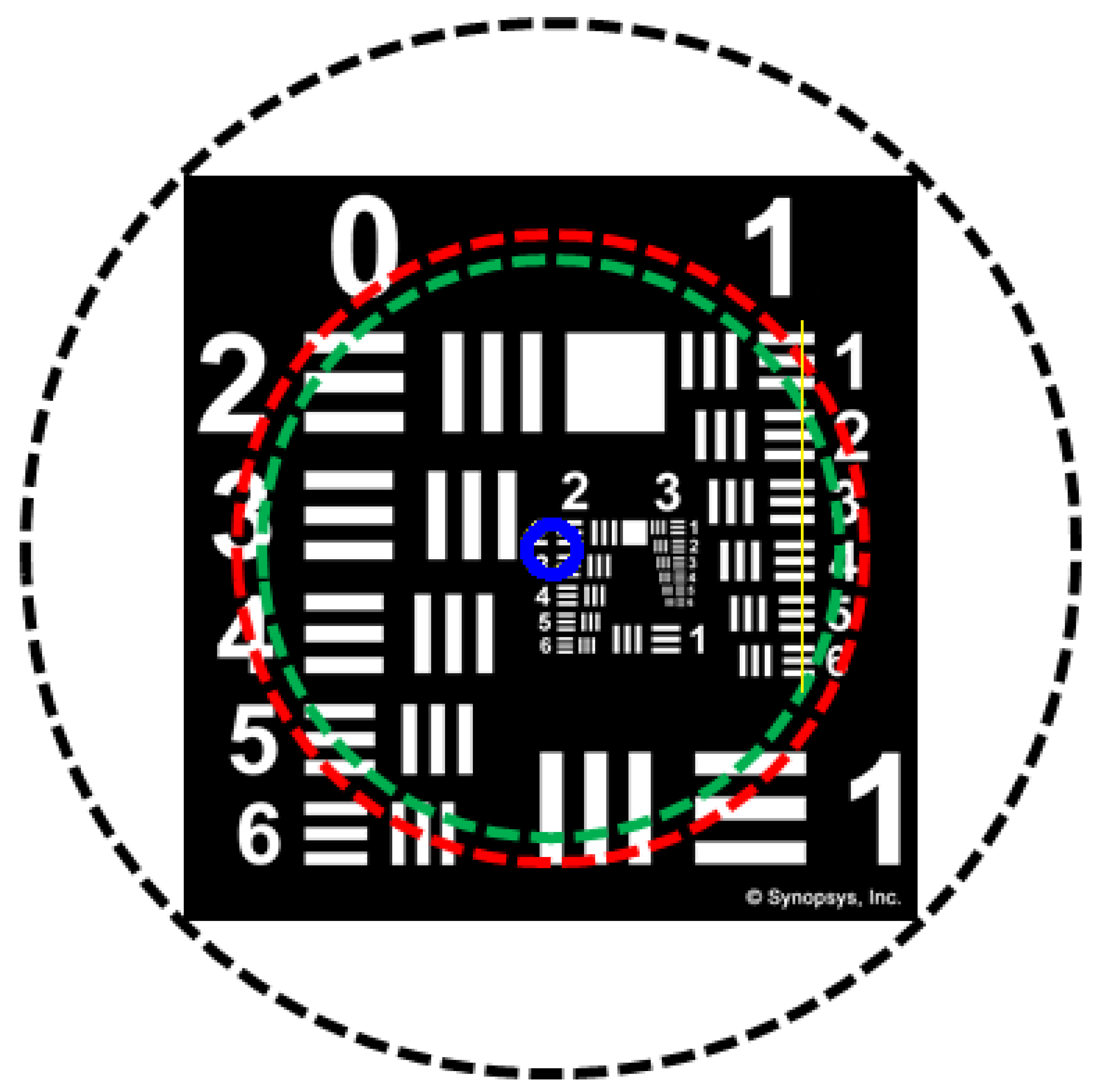
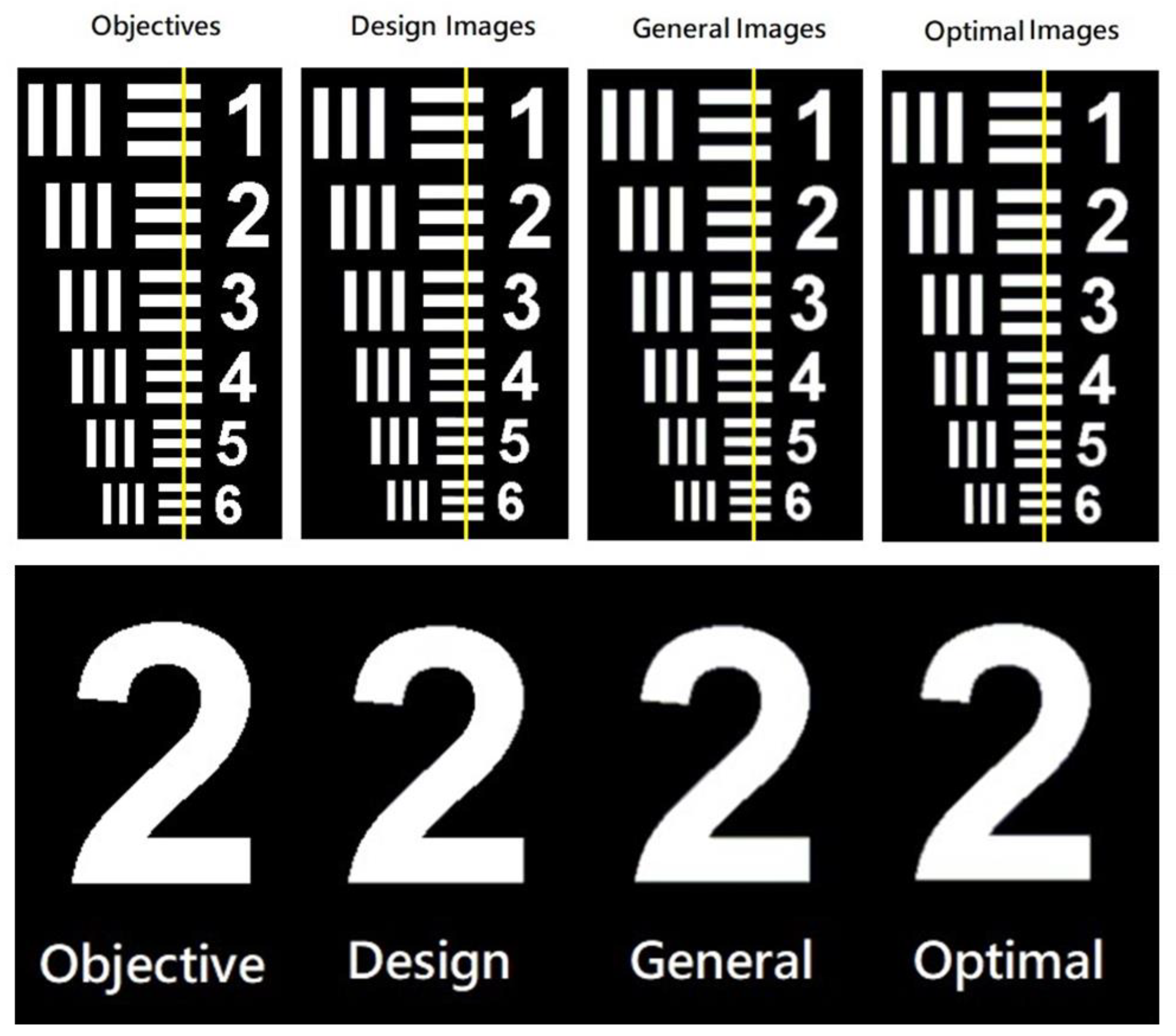
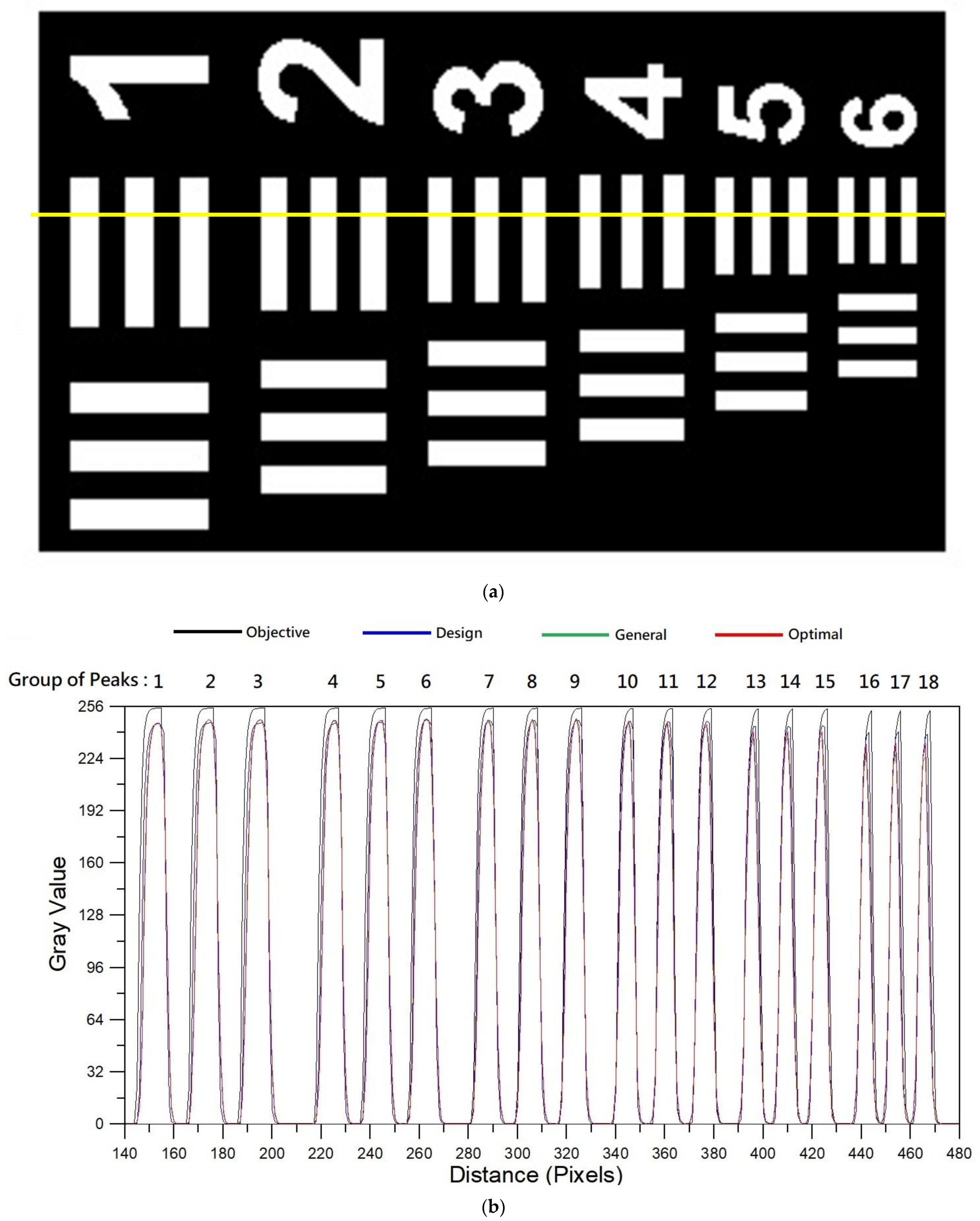
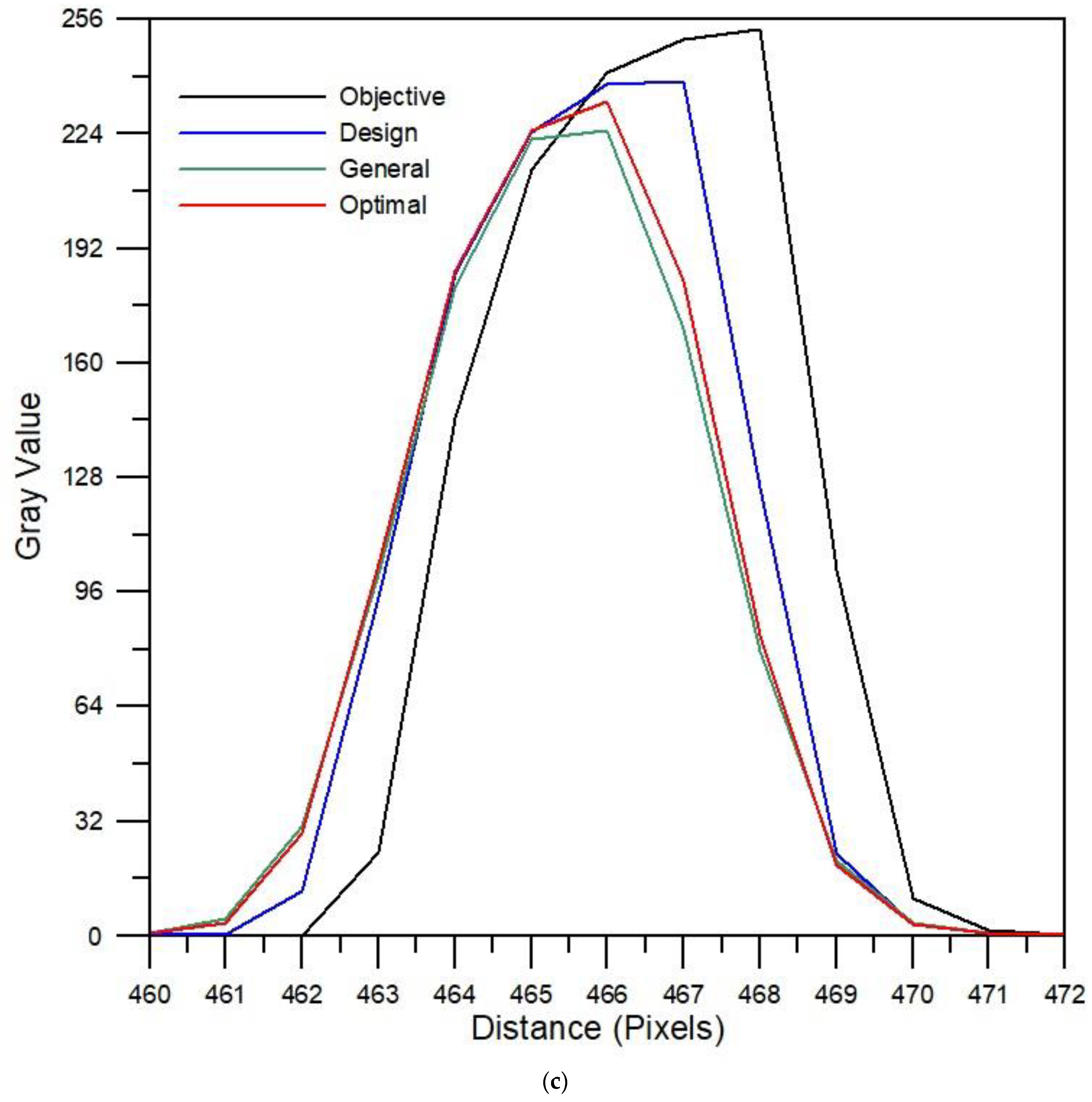
3.4. D Imaging Simulation: Grayscale Analysis of Imaging Quality

The imaging quality of the optimal BTL device was further evaluated by means of grayscale analyses. Figure 13 shows the 1951 USAF resolution test chart commonly used to evaluate the optical imaging quality of lens combinations [25]. Note that the dotted circles correspond to different fields of view (FOVs) with a gradually increasing scale from 0 (blue circle) to 1 (black circle). Figure 14 presents a qualitative comparison of the imaging performance of the ideal (design), general, and optimal BTL designs for the right-hand region of the resolution test chart and numeral “2” in the top-left corner of the chart. Although a slight improvement in the imaging quality is observed for the optimal design, it is unconvincing. Accordingly, quantitative grayscale analysis simulations were conducted along the yellow reference line indicated in the four images in Figure 14 and shown on the right-hand side of Figure 13. As shown in Figure 15a, the analysis was conducted over a distance of 340 pixels, extending from pixel 140 (prior to the first block of three vertical lines in the resolution test chart) to pixel 480 (after the final block of three vertical lines in the test chart). Figure 15b shows the variation in the grayscale intensity along the considered line as observed through the ideal BTL, general BTL, and optimal BTL. In Figure 15b, there are 18 peak groups corresponding to the black and white contrast area of the 18 areas crossed by the yellow line in Figure 15a. The black and white interface is grayscaled due to optical errors and imaging characteristics. These differences can be used to explain the pros and cons of imaging. To better evaluate and compare the imaging qualities of the three BTL designs, the grayscale profiles shown in Figure 15 were partitioned into three sub-profiles corresponding to the 1st peak group, 8th peak group, and 18th peak group in Figure 15. The corresponding results are presented in Figure 16a–c, respectively, where a grayscale curve closer to the objective curve indicates an improved imaging quality (i.e., a lower imaging distortion).
Figure 16 shows that the 1st peak group is the imaging section roughly between pixel distances 143 and 161, the 8th peak group is the imaging section roughly between pixel distances 297 and 313, and the 18th peak group is the imaging section roughly between pixel distances 460 and 472. Observing the three figures, it is clear that the design curve (i.e., the ideal BTL curve) lies closest to the objective curve in all three cases. Moreover, the optimal curve lies closer to the objective curve than the general curve in every case. In other words, the superior imaging quality of the optimized BTL design compared to the general BTL design is confirmed. For the grayscale curves shown in Figure 16a–c, a steeper gradient in the interface regions between the black and white features in the resolution test image implies a greater imaging sharpness. Thus, a detailed inspection of the grayscale analysis results for the optimal and general BTL designs confirms that the optimal design yields a better image sharpness.
The grayscale curves shown in Figure 16a–c correspond to the upper-right, central-right, and lower-right regions of the objective image, respectively (see Figure 13). Comparing the grayscale curves in the three figures, it is seen that the image distortions of the three BTL designs in Figure 16a,c are relatively large and are located to the upper right and lower right of the objective image (see Figure 13), respectively. This result is reasonable since the FOVs are quite large in both cases (i.e., ~0.6 and 0.55, respectively) and the target geometry is not perpendicular to the direction of the FOV, resulting in a larger distortion and asymmetry, respectively. However, the grayscale curves in Figure 16b show both a smaller distortion and a greater symmetry since the FOV is smaller (i.e., 0.45 to 0.5) and the target geometry is perpendicular to the direction of the FOV.

4. Conclusions

This study combined CODE V optical analysis software, the Taguchi experimental design method, and Moldex3D flow analysis simulations to optimize the injection molding processing parameters for a bilateral telecentric lens (BTL) barrel in such a way as to maximize the coaxiality of the tube and improve the imaging performance as a result. The Taguchi analysis results show that a larger maximum packing pressure, a lower melt temperature, and a longer cooling time are all beneficial in improving the coaxiality of the BTL barrel. Moreover, the CODE V and grayscale analysis results show that the BTL barrel molded using the optimal processing conditions yields a better MTF response and focusing performance than a BTL tube molded using the general processing parameters for the chosen polymer material (PA66).

Author Contributions

Conceptualization, C.-M.L., Y.-J.C.; formal analysis, C.-M.L., Y.-J.C.; writing—original draft preparation, C.-M.L., Y.-J.C.; data curation, Y.-J.C.; writing—review and editing, C.-M.L.; supervision, C.-M.L.; funding acquisition, C.-M.L. All authors have read and agreed to the published version of the manuscript.

Funding

This research was funded by the Ministry of Science and Technology of Taiwan, ROC, under Grant Numbers MOST 109-2221-E-415-001-MY3 and MOST 109-2221-E-415-002-MY3.

Institutional Review Board Statement

Not applicable.

Informed Consent Statement

Not applicable.

Acknowledgments

The authors gratefully acknowledge the financial support provided to this study by the Ministry of Science and Technology of Taiwan, ROC.

Conflicts of Interest

The authors declare no conflict of interest.

References

  1. Lin, C.M.; Tan, C.M.; Wang, C.K. Gate design optimization in the injection molding of the optical lens. Optoelectron. Adv. Mater. Rapid Commun. 2013, 7, 580–584. [Google Scholar]
  2. Lin, C.M.; Hsieh, H.K. Processing optimization of Fresnel lenses manufacturing in the injection molding considering birefringence effect. Microsyst. Technol. 2017, 23, 5689–5695. [Google Scholar] [CrossRef]
  3. Lin, C.M.; Chen, Y.W. Grey optimization of injection molding processing of plastic optical lens based on joint consideration of aberration and birefringence effects. Microsyst. Technol. 2019, 25, 621–631. [Google Scholar] [CrossRef]
  4. Lu, X.; Khim, L.S. A statistical experimental study of the injection molding of optical lenses. J. Mater. Process. Technol. 2001, 113, 189. [Google Scholar] [CrossRef]
  5. Lee, Y.B.; Kwon, T.H.; Yoon, K. Numerical prediction of residual stresses and birefringence in injection/compression molded center-gated disk. Part I: Basic modeling and results for injection molding. Polym. Eng. Sci. 2002, 42, 2246–2272. [Google Scholar] [CrossRef]
  6. Shyu, G.D.; Isayyev, A.I.; Lee, H.S. Numerical simulation of flow-induced birefringence in injection molded disk. Jpn. Korea Plast Process Jt. Semin. 2003, 4, 41–47. [Google Scholar]
  7. Fan, B.; Kazmer, D.O.; Bushko, W.C.; Theriault, R.P.; Poslinski, A.J. Birefringence prediction of optical media. Polym. Eng. Sci. 2004, 44, 814–824. [Google Scholar] [CrossRef]
  8. Liao, S.J.; Chang, D.Y.; Chen, H.J.; Tsou, L.S.; Ho, J.R.; Yau, H.T.; Hsieh, W.H.; Wang, J.T.; Su, Y.C. Optimal process conditions of shrinkage and warpage of thin-wall parts. Polym. Eng. Sci. 2004, 44, 917–928. [Google Scholar] [CrossRef]
  9. Tang, S.H.; Tan, Y.J.; Sapuan, S.M.; Sulaiman, S.; Ismail, N.; Samin, R. The use of Taguchi method in the design of plastic injection mould for reducing warpage. J. Mater. Process. Technol. 2007, 182, 418–426. [Google Scholar] [CrossRef]
  10. Bociaga, E.; Jaruga, T.; Lubczynska, K.; Gnatowski, A. Warpage of injection moulded parts as the result of mould temperature difference. Arch. Mat. Sci. Eng. 2010, 44, 28–34. [Google Scholar]
  11. Shayfull, Z.; Ghazali, M.F.; Azaman, M.; Nasir, S.M.; Faris, N.A. Effect of differences core and cavity temperature on injection molded part and reducing the warpage by Taguchi method. Int. J. Eng. Technol. 2010, 10, 125–132. [Google Scholar]
  12. Fischer, R.E.; Tadic-Galeb, B.; Yoder, P.R. Optical System Design, 2nd ed.; McGraw-Hill: New York, NY, USA, 2008; pp. 179–198. [Google Scholar]
  13. Dilworth, D.C. New tools for the lens designer, Current Developments in Lens Design and Optical Engineering IX. Int. Soc. Opt. Photonics 2008, 7060, 70600B. [Google Scholar]
  14. Sahin, F.E. Lens design for active alignment of mobile phone cameras. Opt. Eng. 2017, 56, 065102. [Google Scholar] [CrossRef]
  15. Grabarnik, S. Optical design method for minimization of ghost stray light intensity. Appl. Opt. 2015, 54, 3083–3089. [Google Scholar] [CrossRef]
  16. Sahin, F.E. Open-source optimization algorithms for optical design. Optik 2019, 178, 1016–1022. [Google Scholar] [CrossRef]
  17. Houllier, T.; Lépine, T. Comparing optimization algorithms for conventional and freeform optical design: Erratum. Opt. Express 2019, 27, 28383. [Google Scholar] [CrossRef]
  18. Lin, C.M.; Chen, Y.J. Taguchi Optimization of Roundness and Concentricity of a Plastic Injection Molded Barrel of a Telecentric Lens. Polymers 2021, 13, 3419. [Google Scholar] [CrossRef]
  19. Sui, W.; Zhang, D. Four Methods for Roundness Evaluation. Phys. Procedia 2012, 24, 2159–2164. [Google Scholar] [CrossRef] [Green Version]
  20. Ahn, S.J. Least Squares Orthogonal Distance Fitting of Curves and Surfaces in Space; Springer: Berlin/Heidelberg, Germany, 2004. [Google Scholar]
  21. Srinivasan, V.; Shakarji, C.M.; Morse, E.P. On the enduring appeal of least-squares fitting in computational coordinate metrology. J. Comput. Inf. Sci. Eng. 2011, 12, 011008. [Google Scholar] [CrossRef]
  22. Kim, N.H.; Kim, S.W. Geometrical tolerances: Improved linear approximation of least-squares evaluation of circularity by minimum variance International. J. Mach. Tools Manuf. 1996, 36, 355–366. [Google Scholar] [CrossRef]
  23. Hichem, N.; Pierre, B. Evaluation of roundness error using a new method based on a small displacement screw. Meas. Sci. Technol. 2014, 25, 25. [Google Scholar]
  24. O’Shea, D.C.; Bentley, J.L. Designing Optics Using CODE V; SPIE PRESS: Bellingham, WA, USA, 2018. [Google Scholar]
  25. MIL-STD-150A; Military Standard: Photographic Lenses. EverySpec LLC: Gibsonia, PA, USA, 12 May 1959.
Figure 1. Geometry and optical design of the BTL (unit: mm).
Symmetry 14 00200 g001
Figure 2. Flow chart showing the main steps in the optical design and injection molding optimization procedure for the BTL.
Symmetry 14 00200 g002
Figure 3. (a) Viscosity and (b) P-v-T properties of PA66 material (source: Moldex3D material library).
Symmetry 14 00200 g003
Figure 4. (a) Injection molding system and (b) cooling system of the BTL (D: diameter; L: length; unit: mm).
Symmetry 14 00200 g004aSymmetry 14 00200 g004b
Figure 5. Considering the processing factors (maximum injection pressure and maximum packing pressure), the real sprue pressure change and flow rate change presented by the general design and the optimal design during the filling stage and the packing stage are shown.
Symmetry 14 00200 g005
Figure 6. Coaxiality and S/N values for different control factor level settings in Moldex3D simulations.
Symmetry 14 00200 g006
Figure 7. Center distribution and concentricity values in the design, general, and optimal BTL models.
Symmetry 14 00200 g007
Figure 8. Modulation vs. spatial frequency response for different light fields in the design, general, and optimal BTL models.
Symmetry 14 00200 g008
Figure 9. MTF for light field I in the design, general, and optimal BTL models.
Symmetry 14 00200 g009
Figure 10. MTF for light field II in the design, general, and optimal BTL models.
Symmetry 14 00200 g010
Figure 11. MTF for light field III in the design, general, and optimal BTL models.
Symmetry 14 00200 g011
Figure 12. Spot diagrams of three light fields in the design, general, and optimal BTL models.
Symmetry 14 00200 g012
Figure 13. 1951 USAF resolution test chart with graduated FOV. Black circle: FOV = 1; red circle: FOV = 0.6; green circle: FOV = 0.55; blue circle: FOV = 0. Yellow line shows reference line used to examine image distortion and sharpness of different BTL designs by grayscale analysis.
Symmetry 14 00200 g013
Figure 14. Two-dimensional image simulation results for the design, general, and optimal BTL models.
Symmetry 14 00200 g014
Figure 15. Quantitative image distortion and sharpness evaluation of objective, design, general, and optimal BTL models. (a) Analysis region in the USAF resolution test chart (refer to Figure 12, rotate 90 degrees counterclockwise). (b) Variation in grayscale intensity with pixel distance along yellow reference line.
Symmetry 14 00200 g015
Figure 16. (a) Variation in grayscale intensity over pixel range of 143–161 (peak group 1 in Figure 15b). (b) Variation in grayscale intensity over pixel range of 297–313 (peak group 8 in Figure 15b). (c) Variation in grayscale intensity over pixel range of 460–472 (peak group 18 in Figure 15b).
Symmetry 14 00200 g016aSymmetry 14 00200 g016bSymmetry 14 00200 g016c
Table 1. Material properties and recommended processing conditions for PA66 (TECHNYL A 216, Solvay Engineering Plastics).
Material PropertiesValuesUnit
Density1140Kg/m3
Specific heat2 × 10−11J/Kg. °C
Heat conduction coefficient0.25J/s.m. °C
Mold shrinkage1.90%
Tensile modulus3000MPa
Melt temperature263°C
Coefficient of linear thermal expansion (23–85 °C)7 × 10⁻⁵°C
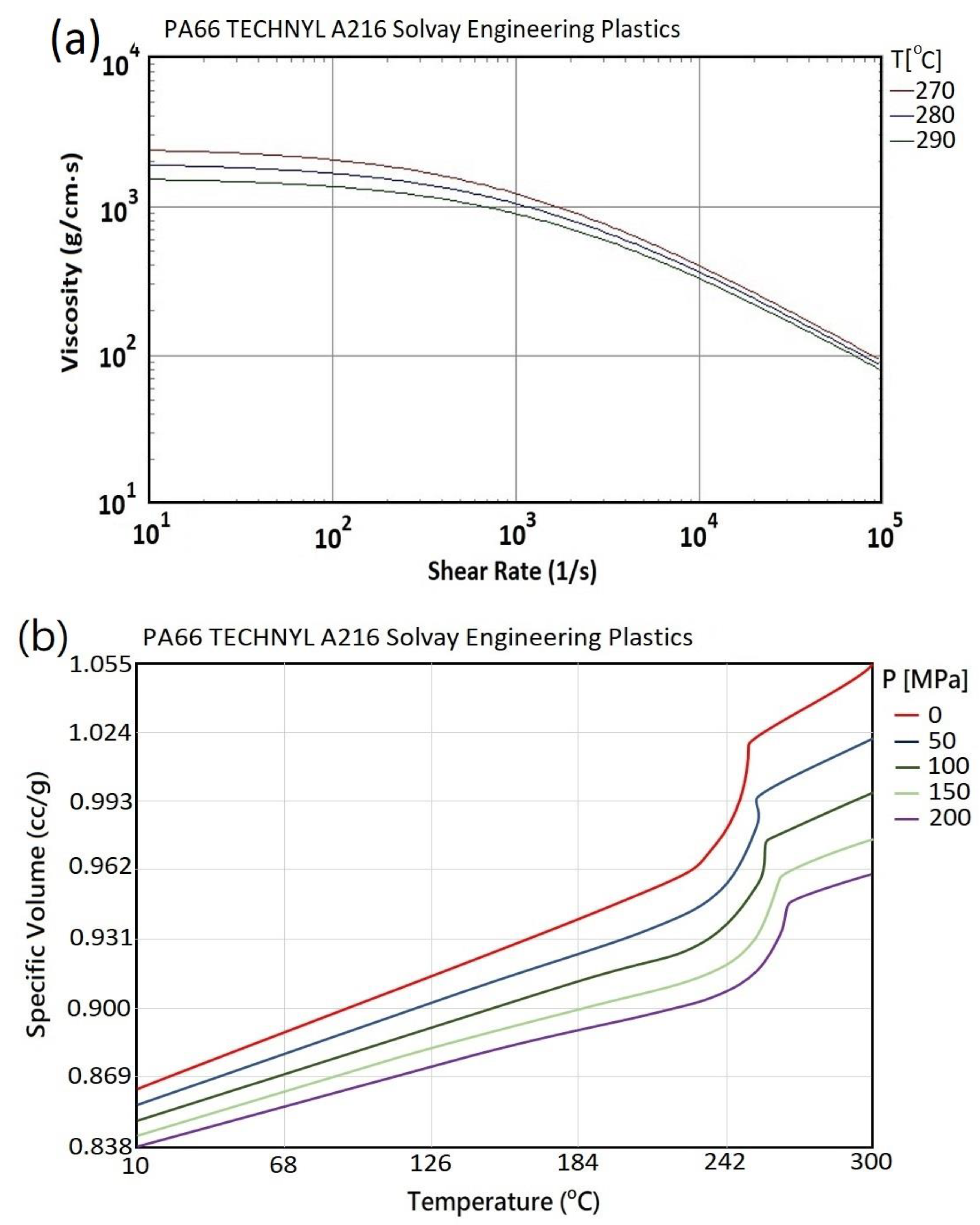
Viscosity vs. shear rate under different temperaturesshown in Figure 3a
P-v-Tshown in Figure 3b
Processing Conditions in Injection Molding (Recommended)ValuesUnit
Maximum injection pressure180–240MPa
Maximum packaging pressure180–240MPa
Melt temperature270–290°C
Mold temperature60–100°C
Cooling time11–17s
Ejection temperature190°C
Curing temperature210°C
Table 2. Optical properties and geometrical dimensions of lenses in the BTL.
Lens No.Glass/SCHOTTCurvature Radius
(mm)
Thickness
(mm)
Refractive Index
(-)
Abbe Value
(-)
Partial Dispersion
(-)
Dispersion (NL-N1)
(-)
Len 1NLAK33A109.20835.00651.7539352.2710.303230.01442
−786.0770
Len 2NLAK33B38.82835.00441.7550052.3000.303210.01444
137.9732
Len 3FK5HTI−67.991418.19441.4874870.4700.309770.00692
15.3674
Len 4LAFN7427.953417.21651.7495034.9510.294140.02144
−33.0637
Table 3. Taguchi L16(54) orthogonal array for coaxiality optimization of the BTL.
TrialsProcessing Factors
A
Maximum
Injection
Pressure
(MPa)
B
Maximum
Packing
Pressure
(MPa)
C
Melt
Temperature (°C)
D
Mold
Temperature
(°C)
E
Cooling
Time
(s)
General Parameters2002002808013
11801802757011
21802002808013
31802202859015
418024029010017
52001802809017
620020027510015
72002202907013
82002402858011
922018028510013
102202002909011
112202202758017
122202402807015
132401802908015
142402002857017
1524022028010011
162402402759013
Optimal Parameters 2202402759017
Table 4. Signal-to-noise (S/N) response of control factors and level settings.
FactorControl Factors
Level/
Range/Rank
ABCDE
Level 1 (dB)18.4242617.9307418.6493418.433218.38978
Level 2 (dB)18.4400418.2959818.5156218.4585218.36406
Level 3 (dB)18.471418.6306618.382218.4524718.44444
Level 4 (dB)18.449118.9274118.2376518.4406118.58652
S/N Range (dB)0.0471420.9966630.411690.0253220.22246
Influence Rank41253
Table 5. Injection molding process parameters for general design and optimal design.
General DesignOptimal Design
         Filling
Filling time (s)2.132.13
Melt temperature (°C)280275
Mold temperature (°C)8090
Maximum injection pressure (MPa)200220
Injection volume (cm3)68.168.1
         Packing
Packing time (s)77
Maximum packing pressure (MPa)200240
         Cooling
Cooling time (s)1317
Mold-open time (s)55
Eject temperature (°C)190190
Air temperature (°C)2525
         Miscellaneous
Cycle time (s)27.1327.13
Table 6. Center coordinates/concentricity values of four reference planes and coaxiality of the optical tube in the design, general, and optimal BTL models.
Unit: mmDesignGeneralOptimal
Planes Center   Coordinate   Bias :   Z i ( Δ Xc ,   Δ Yc ,   Δ Zc ) ; Concentricity = d i   ( i = 1 4 ) ( mm ) ;   Coaxiality = i = 1 4 ( d i ) 2 / 4 ( mm 2 )
Z1 = 0(0, 0, 0)
0
Z1(0.173964, −0.000240496, 0.937954)
d1 = 0.173964166
Z1(0.152848, −0.000185194, 0.728356)
d1 = 0.152848112
Z2 = 57.75(0, 0, 0)
0
Z2(−0.00609915, −0.000210664, 0.162)
d2 = 0.006102787
Z2(−0.0169768, −0.000159105, 0.1405)
d2 = 0.016977546
Z3 = 82.3(0, 0, 0)
0
Z3(−0.0546394, −0.00013, −0.1749)
d3 = 0.0546394
Z3(−0.0581023, −0.0000981, −0.127)
d3 = 0.058102383
Z4 = 117.7(0, 0, 0)
0
Z4(0.161799, −0.000609249, −0.662)
d4 = 0.1618
Z4(0.140132, −0.000555817, −0.52)
d4 = 0.140133102
Coaxiality00.0148660.011666
Publisher’s Note: MDPI stays neutral with regard to jurisdictional claims in published maps and institutional affiliations.

