An Approximate Solution for the Contact Problem of Profiles Slightly Deviating from Axial Symmetry

Abstract

An approximate solution for a contact problem of profiles which are not axially symmetrical but deviate only slightly from the axial symmetry is found in a closed explicit analytical form. The solution is based on Betti’s reciprocity theorem, first applied to contact problems by R.T. Shield in 1967, in connection with the extremal principle for the contact force found by J.R. Barber in 1974 and Fabrikant’s approximation (1986) for the pressure distribution under a flat punch with arbitrary cross-section. The general solution is validated by comparison with the Hertzian solution for the contact of ellipsoids with small eccentricity and with numerical solutions for conical shapes with polygonal cross-sections. The solution provides the dependencies of the force on the indentation, the size and the shape of the contact area as well as the pressure distribution in the contact area. The approach is illustrated by linear (conical) and quadratic profiles with arbitrary cross-sections as well as for “separable” shapes, which can be represented as a product of a power-law function of the radius with an arbitrary exponent and an arbitrary function of the polar angle. A generalization of the Method of Dimensionality Reduction to non-axisymmetric profiles is formulated.

1. Introduction

In 1882, Heinrich Hertz solved the problem of elastic contact of parabolic bodies [1]. A solution for the contact of an arbitrary body of revolution with a compact contact area was found much later, in 1941–1942 by Föppl and Schubert [2,3,4]. An attempt to overcome the restriction of axial symmetry was undertaken in 1990 by Barber and Billings [5]. Their approach is based on using Betti’s reciprocity theorem as suggested by Shield in 1967 [6] and the extremal principle found by Barber [7]. However, in [5] Barber and Billings merely illustrated their method on examples of contacts with “linear profiles” (pyramids with polygonal cross-sections) since an analytical solution is possible only for this case. In the present paper, we apply the extremal principle of Barber to another case where a largely analytical treatment is possible: To contacts of profiles that are not axially symmetrical but deviate only slightly from the axial symmetry.

2. Barber’s Extremal Principle

In [6], Shield used Betti’s reciprocity theorem to show that the normal force $F_N(A)$ appearing due to indentation of the profile $f(x,y)$ to a depth $d$ (while $A$ is the contact area in this state) is given by the equation

$$F_N(A)=\frac{1}{d^{*}}{\displaystyle {\iint }_A{p}^{*}(x,y)\left(d-f(x,y)\right)\mathrm{d}x\mathrm{d}y}$$

(1)

where in the pressure distribution, $p^{*}(x,y)$ is that under a flat punch with the cross-sectional shape $A$ which is indented by $d^{*}$. Note that the indentation $d^{*}$ is an auxiliary parameter used solely for determining the pressure $p^{*}(x,y)$; it has nothing to do with the true indentation depth d. Of course, the integral (1) does not depend on $d^{*}$ as pressure $p^{*}(x,y)$ under an arbitrary flat punch is proportional to $d^{*}$. In [7], Barber has shown that the area $A$ fulfilling the usual contact conditions (the pressure inside the contact area is positive and there is no interpenetration, outside the contact, the pressure is zero and the distance between surfaces is positive), corresponds to the maximum force at a given indentation depth. (For axisymmetric profiles, this extremal principle has already been used by Shield [6]).

To be able to look constructively for a solution, Barber and Billings propose to use Fabrikant’s approximation [8] for the pressure distribution under a flat-ended punch. Fabrikant’s hypothesis is that the stress distribution is given in a good approximation by the equation

$$p=\frac{2E^{*}d}{L}\frac{a(\phi )}{\sqrt{a{(\phi )}^2-r^2}}$$

(2)

where $a(\phi )$ is the equation for the contact boundary in polar coordinates and

$$L={\displaystyle \underset{0}{\overset{2\pi }{\int }}a(\phi )\mathrm{d}\phi }$$

(3)

The motivation for the ansatz (2) is straightforward. It is known to be exact for elliptical punches with arbitrary eccentricity, and it provides the correct kind of asymptotic behavior in the vicinity of the boundary, which must be fulfilled for a flat-ended punch of arbitrary shape [9].

The origin for the polar coordinate system has to be taken as the centroid of the area A provided there are no tilting moments around the origin (which we will assume in this paper).

With Fabrikant’s pressure (2), Equation (1) becomes

$$F_N(A)=\frac{2E^{*}}{L}{\displaystyle \underset{0}{\overset{2\pi }{\int }}{\displaystyle \underset{0}{\overset{a(\phi )}{\int }}\frac{a(\phi )\left(d-f(r,\phi )\right)r\mathrm{d}r\mathrm{d}\phi }{\sqrt{a{(\phi )}^2-r^2}}}}$$

(4)

Introducing definitions

$$g_{\phi }(a)=a{\displaystyle \underset{0}{\overset{a}{\int }}\frac{f^{\prime }\left(r,\phi \right)}{\sqrt{a^2-r^2}}\mathrm{d}r},\frac{\mathrm{d}{G}_{\phi }(a)}{\mathrm{d}a}=g_{\phi }(a),$$

(5)

the force (4) can be rewritten as

$$F_N(A)=\frac{2E^{*}}{L}{\displaystyle \underset{0}{\overset{2\pi }{\int }}\left(d\cdot a{(\phi )}^2-a(\phi )G_{\phi }(a(\phi ))\right)\mathrm{d}\phi }$$

(6)

3. Finding the Force Maximum

3.1. Axially Symmetric Profiles

In the case of an axially symmetric profile, $a(\phi )=a_0$, $L=2\pi a_0$, the force equation simplifies to

$$F_N(a_0)=2E^{*}\left(d\cdot a_0-G(a_0)\right)$$

(7)

The condition for its maximum reads $\mathrm{d}{F}_N(a_0)/\mathrm{d}{a}_0=2E^{*}\left(d-g(a_0)\right)=0$ or

$$d=g(a_0)$$

(8)

and the normal force is equal to

$$F_N(a_0)=E^{*}{\displaystyle \underset{-a_0}{\overset{a_0}{\int }}\left(d_0-g(a)\right)}\mathrm{d}a$$

(9)

The pressure distribution can be calculated by integrating contributions (2) during indentation from the first touch up to the given indentation depth, as described in detail in [10] (Appendix B),

$$p(r)=\frac{E^{*}}{\pi }{\displaystyle \underset{r}{\overset{a}{\int }}\frac{1}{\sqrt{{\tilde{a}}^2-r^2}}}\frac{\mathrm{d}g(\tilde{a})}{\mathrm{d}\tilde{a}}\mathrm{d}\tilde{a}$$

(10)

Equations (8)–(10) are the well-known equations of the Method of Dimensionality Reduction (MDR) [11].

3.2. General Profiles

In the general case of non-axisymmetric profiles, let us first search for the maximum of functional (6) at a constant value of $L$. This can be done, according to Lagrange, by searching for an unconditional extremum of the functional

$$\frac{2E^{*}}{L}{\displaystyle \underset{0}{\overset{2\pi }{\int }}\left(d\cdot a{(\phi )}^2-a(\phi )G_{\phi }(a(\phi ))\right)\mathrm{d}\phi }-D\left({\displaystyle \underset{0}{\overset{2\pi }{\int }}a(\phi )\mathrm{d}\phi -L}\right)$$

(11)

where $D$ is a Lagrange multiplier. At the maximum of this functional, the first variation must vanish identically

$$\frac{2E^{*}}{L}\left(2d\cdot a(\phi )-G_{\phi }(a(\phi ))-a(\phi )g_{\phi }(a(\phi ))\right)=D$$

(12)

This equation determines implicitly the contact boundary $a(\phi )$, while $D$ is connected with $L$ through the condition (3). After substitution of $a(\phi )$ into (6), the force will remain a function of the still undefined L, which should finally be found as a value giving the maximum to the force. All stated operations, beginning with the solution of Equation (12) with respect to $a(\phi )$, can be carried out analytically without approximations only in two cases: Either the above case of axisymmetric profiles (leading to the MDR) or in the case of linear (conical) profiles. The latter has already been done in the paper [5] for polygonal cross-sections. To be able to constructively realize the above program for more general shapes, let us consider profiles that only slightly deviate from axisymmetric ones. We will show below that this is the third case where a largely analytical treatment is possible.

3.3. Profiles Slightly Deviating from Axisymmetric Ones

Let us consider a profile that is not axially symmetrical but deviates only slightly from axial symmetry:

$$f(r,\phi )=f_0(r)+\delta f(r,\phi )$$

(13)

where $\delta f(r,\phi )$ is a small deviation. We define the position of the origin of coordinates in such a way that

$$f(0,\phi )=f_0(0)=\delta f(0,\phi )=0$$

(14)

The functions $g_{\phi }(a)$ and $G_{\phi }(a)$ will correspondingly consist of two parts

$$G_{\phi }(a)=G_0(a)+\delta G_{\phi }(a),g_{\phi }(a)=g_0(a)+\delta g_{\phi }(a),g_{\phi }{}^{\prime }(a)=g_0{}^{\prime }(a)+\delta g_{\phi }{}^{\prime }(a)$$

(15)

with

$$g_0(a)=a{\displaystyle \underset{0}{\overset{a}{\int }}\frac{f_0{}^{\prime }\left(r\right)}{\sqrt{a^2-r^2}}\mathrm{d}r},\delta g_{\phi }(a)=a{\displaystyle \underset{0}{\overset{a}{\int }}\frac{\delta f_0{}^{\prime }\left(r,\phi \right)}{\sqrt{a^2-r^2}}\mathrm{d}r}$$

(16)

and correspondingly

$$G_0{}^{\prime }(a)=g_0(a),\delta {G^{\prime }}_{\phi }(a)=\delta g_{\phi }(a)$$

(17)

The contact boundary will also be almost a circle with a small perturbation

$$a(\phi )=a_0+\delta a(\phi )$$

(18)

Substituting (18) into (12), expanding all functions with respect to small deviation $\delta a(\phi )$ and neglecting all terms of the second or higher orders, we get for the deviation of the contact contour from a circle in the first approximation

$$\delta a(\phi )=\frac{\frac{D\pi a_0}{E^{*}}-2d{a}_0+G_{\phi }(a_0)+a_0{g}_{\phi }(a_0)}{2d-2g_{\phi }(a_0)-a_0{g}_{\phi }{}^{\prime }(a_0)}$$

(19)

With (15), we obtain

$$\begin{array}{l}\delta a(\phi ){\left[2d-2g_0(a_0)-a_0{g}_0{}^{\prime }(a_0)\right]}^2\\ =\left[\frac{D\pi a_0}{E^{*}}-2d{a}_0+G_0(a_0)+a_0{g}_0(a_0)\right]\left[2d-2g_0(a_0)-a_0{g}_0{}^{\prime }(a_0)\right]\\ +\left[2d-2g_0(a_0)-a_0{g}_0{}^{\prime }(a_0)\right]\left[\delta G_{\phi }(a_0)+a_0\delta g_{\phi }(a_0)\right]\\ +\left[\frac{D\pi a_0}{E^{*}}-2d{a}_0+G_0(a_0)+a_0{g}_0(a_0)\right]\left[2\delta g_{\phi }(a_0)-a_0\delta g_{\phi }{}^{\prime }(a_0)\right]\end{array}$$

(20)

To determine the Lagrange multiplier $D$ we require

$${\displaystyle \underset{0}{\overset{2\pi }{\int }}\delta a(\phi )\mathrm{d}\phi }=0$$

(21)

Note that the separation (13) into an axisymmetric part and perturbation is not unique. We can use this freedom to essentially simplify the following relations. Let us define the deviation in such a way that

$${\displaystyle \underset{0}{\overset{2\pi }{\int }}\delta g_{\phi }(a_0)\mathrm{d}\phi }=0$$

(22)

for all $a_0$. This will automatically mean that

$${\displaystyle \underset{0}{\overset{2\pi }{\int }}\delta G_{\phi }(a_0)\mathrm{d}\phi }=0\mathrm{and}{\displaystyle \underset{0}{\overset{2\pi }{\int }}\delta g_{\phi }{}^{\prime }(a_0)\mathrm{d}\phi }=0$$

(23)

and also guarantee that

$${\displaystyle \underset{0}{\overset{2\pi }{\int }}\left[\delta G_{\phi }(a_0)+a_0\delta g_{\phi }(a_0)\right]\mathrm{d}\phi }=0$$

(24)

and thus, that integral over $\phi$ of the term in the third line in (20) vanishes. If we now chose the constant $D$ such that $\left[\frac{D\pi a_0}{E^{*}}-2d{a}_0+G_0(a_0)+a_0{g}_0(a_0)\right]=0$, then the integrals over $\phi$ of the terms in the second and fourth lines of (20) vanish identically and the condition (21) is fulfilled. We then obtain from (20)

$$\delta a(\phi )=\frac{\left[\delta G_{\phi }(a_0)+a_0\delta g_{\phi }(a_0)\right]}{\left[2d-2g_0(a_0)-a_0{g}_0{}^{\prime }(a_0)\right]}$$

(25)

The force (6) can now be written as

$$\begin{array}{l}{F}_N(A)=\frac{E^{*}}{\pi a_0}{\displaystyle \underset{0}{\overset{2\pi }{\int }}\left(d\cdot a{(\phi )}^2-a(\phi )G_{\phi }(a(\phi ))\right)\mathrm{d}\phi }\\ =\frac{E^{*}}{\pi a_0}{\displaystyle \underset{0}{\overset{2\pi }{\int }}\left(d\cdot a_0{}^2-a_0{G}_0(a_0)\right)\mathrm{d}\phi }+\frac{E^{*}}{\pi a_0}{\displaystyle \underset{0}{\overset{2\pi }{\int }}\left[2d\cdot a_0-G_0(a_0)-a_0{g}_0(a_0)\right]\delta a(\phi )\mathrm{d}\phi }-\frac{E^{*}}{\pi }{\displaystyle \underset{0}{\overset{2\pi }{\int }}\delta G_{\phi }(a_0)\mathrm{d}\phi }\end{array}$$

(26)

The second and the third term are equal to zero due to relations (22) and (23) so that only the first term remains. Its maximization leads to the usual MDR result [11]

$$d=g_0(a_0)$$

(27)

This means that Equation (25) can finally be rewritten as follows:

$$\delta a(\phi )=-\frac{\delta G_{\phi }(a_0)+a_0\delta g_{\phi }(a_0)}{a_0{g}_0{}^{\prime }(a_0)}$$

(28)

This equation provides the explicit solution for the deviation of the contact boundary from the circle with radius $a_0$. The normal force is given by the Equation (9)

$$F_N(a_0)=2E^{*}{\displaystyle \underset{0}{\overset{a_0}{\int }}\left(d-g_0(a)\right)}\mathrm{d}a$$

(29)

3.4. Pressure Distribution for Profiles Slightly Deviating from Axisymmetric Ones

Let us take a close look at the process of indentation from the first touch to the final indentation depth $d$ and denote the current values of the force, the indentation depth and the effective contact radius respectively by ${\tilde{F}}_N$, $\tilde{d}$ and ${\tilde{a}}_0$. The entire process consists of changing the indentation depth from $\tilde{d}=0$ to $\tilde{d}=d$, whereby the contact radius changes from $\tilde{a}=0$ to ${\tilde{a}}_0=a_0$ and the contact force from ${\tilde{F}}_N=0$ to ${\tilde{F}}_N=F_N$. An infinitesimal indentation by $\mathrm{d}\tilde{d}$ of the area, which is given by the contour equation $r=a(\phi )$, produces the following contribution to the pressure distribution

$$\mathrm{d}p=\frac{E^{*}}{\pi a_0}\frac{a(\phi )}{\sqrt{a{(\phi )}^2-r^2}}\mathrm{d}\tilde{d}\mathrm{for}r<a(\phi )$$

(30)

The pressure distribution at the end of the indentation process is equal to the sum of the incremental pressure distributions:

$$p(r,\phi )=\frac{E^{*}}{\pi }{\displaystyle \underset{d\left(r\right)}{\overset{d}{\int }}\frac{1}{{\tilde{a}}_0}\frac{\tilde{a}(\phi )}{\sqrt{\tilde{a}{(\phi )}^2-r^2}}\mathrm{d}\tilde{d}}=\frac{E^{*}}{\pi }{\displaystyle \underset{r}{\overset{a(\phi )}{\int }}\frac{1}{\sqrt{\tilde{a}{(\phi )}^2-r^2}}}\frac{\tilde{a}(\phi )}{{\tilde{a}}_0}\frac{\mathrm{d}{g}_0({\tilde{a}}_0)}{\mathrm{d}\tilde{a}(\phi )}\mathrm{d}\tilde{a}(\phi )$$

(31)

where ${\tilde{a}}_0$ must be considered here as a function of $\tilde{a}(\phi )$.

4. Examples

4.1. Contact with Parabolic Profiles with Arbitrary Cross-Section

Consider a profile

$$z=f(r,\phi )=r^2\psi (\phi )$$

(32)

Thus

$$f_0(r)=r^2\overline{\psi }\mathrm{and}\delta f(r,\phi )=r^2\left(\psi (\phi )-\overline{\psi }\right)$$

(33)

where $\overline{\psi }$ is the averaged value of $\psi (\phi )$ over all angles:

$$\overline{\psi }=\frac{1}{2\pi }{\displaystyle \underset{0}{\overset{2\pi }{\int }}\psi (\phi )\mathrm{d}\phi }$$

(34)

The corresponding angle-dependent “MDR profile” is

$$g_{\phi }(a)=2a^2\psi (\phi )$$

(35)

For all necessary auxiliary functions, we get

$$g_0(a)=2\overline{\psi }{a}^2,\delta g_{\phi }(a)=2a^2\left(\psi (\phi )-\overline{\psi }\right),g_0{}^{\prime }(a)=4\overline{\psi }a,$$

(36)

$$G_0(a)=\frac{2\overline{\psi }{a}^3}{3},\delta G_{\phi }(a)=\frac{2a^3}{3}\left(\psi (\phi )-\overline{\psi }\right).$$

(37)

The effective contact radius is given by Equation (27):

$$a_0=\sqrt{\frac{d}{2\overline{\psi }}}$$

(38)

and the contact area is given by the relation (18)

$$a(\phi )=a_0\left(\frac{5}{3}-\frac{2}{3}\frac{\psi (\phi )}{\overline{\psi }}\right)$$

(39)

To find the pressure distribution, we use Equation (31)

$$p(r,\phi )=\frac{E^{*}}{\pi }{\displaystyle \underset{r}{\overset{a(\phi )}{\int }}\frac{\tilde{a}(\phi )}{\sqrt{\tilde{a}{(\phi )}^2-r^2}}}\frac{1}{{\tilde{a}}_0}\frac{\mathrm{d}{g}_0({\tilde{a}}_0)}{\mathrm{d}\tilde{a}(\phi )}\mathrm{d}\tilde{a}(\phi )=\frac{2}{\pi }{E}^{*}{\left(2d\cdot \overline{\psi }\right)}^{1/2}\sqrt{1-{\left(\frac{r}{a(\phi )}\right)}^2}$$

(40)

4.2. Contact with a Paraboloid

As a special case of a general parabolic profile, let us consider a paraboloid

$$z=f(x,y)=\frac{x^2}{2R_1}+\frac{y^2}{2R_2}=\frac{r^2}{2}\left(\frac{{\cos }^2\phi }{R_1}+\frac{{\sin }^2\phi }{R_2}\right)$$

(41)

In this case,

$$\psi (\phi )=\frac{1}{2}\left(\frac{{\cos }^2\phi }{R_1}+\frac{{\sin }^2\phi }{R_2}\right)=\frac{1}{4}\left(\frac{1}{R_1}+\frac{1}{R_2}\right)+\frac{1}{4}\left(\frac{1}{R_1}-\frac{1}{R_2}\right)\cos 2\phi$$

(42)

and

$$\overline{\psi }=\frac{1}{4}\left(\frac{1}{R_1}+\frac{1}{R_2}\right)$$

(43)

Equations (38)–(40) take the form

$$a_0=\sqrt{\frac{2d\cdot R_1{R}_2}{R_1+R_2}}$$

(44)

$$a(r,\phi )=a_0\left[1-\frac{2}{3}\frac{R_2-R_1}{R_1+R_2}\cos 2\phi \right]$$

(45)

and

$$p(r,\phi )=\frac{2}{\pi }{E}^{*}{\left(\frac{d\cdot (R_1+R_2)}{2R_1{R}_2}\right)}^{1/2}\sqrt{1-{\left(\frac{r}{a(\phi )}\right)}^2}$$

(46)

The total normal force is equal to

$$F_N=\frac{4}{3}{E}^{*}{\left(\frac{2R_1{R}_2}{R_1+R_2}\right)}^{1/2}{d}^{3/2}\left(1-{\left(\frac{2}{3}\frac{R_2-R_1}{R_1+R_2}\right)}^2\right)$$

(47)

Equation (45) describes in the approximation of small eccentricities an ellipse with half-axes

$$a=a_0\left[1+\frac{2}{3}\frac{R_2-R_1}{R_1+R_2}\right],\mathrm{and}b=a_0\left[1-\frac{2}{3}\frac{R_2-R_1}{R_1+R_2}\right]$$

(48)

For the eccentricity of the contact area, we get

$$e=\sqrt{1-\frac{b^2}{a^2}}=\frac{2}{\sqrt{3}}{e}_g\frac{\sqrt{1-e_g^2/2}}{1-e_g^2/6}$$

(49)

where

$$e_g=\sqrt{1-\frac{R_1}{R_2}}$$

(50)

is the eccentricity of cross-sections of the indenter. For small eccentricities, the ratio of eccentricities of contact area and cross-sections of the ellipsoid is constant and equal to $2/\sqrt{3}$, which is the exact asymptotic value according to the Hertzian solution [9] (p. 35). Equation (49) provides a very good approximation for the exact solution for eccentricities up to 0.7 (see Figure 1).

4.3. Contact of a Conical Indenter with an Arbitrary Cross-Section

Consider a general conical profile with an “almost axisymmetric” shape

$$f(r,\phi )=r\cdot \psi (\phi )=f_0(r)+\delta f(r,\phi )$$

(51)

Thus

$$f_0(r)=r\overline{\psi }\mathrm{and}\delta f(r,\phi )=r\left(\psi (\phi )-\overline{\psi }\right)$$

(52)

where $\overline{\psi }$ is the averaged value of $\psi (\phi )$ over all angles according to (34). For all necessary auxiliary functions, we get

$$g_0(a)=\frac{\pi }{2}a\overline{\psi },\delta g_{\phi }(a)=\frac{\pi }{2}a\left(\psi (\phi )-\overline{\psi }\right),g_0{}^{\prime }(a)=\frac{\pi }{2}\overline{\psi }$$

(53)

$$G_0(a)=\frac{\pi }{4}{a}^2\overline{\psi },\delta G_{\phi }(a)=\frac{\pi }{4}{a}^2\left(\psi (\phi )-c\right)$$

(54)

The contact area is given by the relation (18)

$$a(\phi )=\frac{2}{\pi }\frac{d}{\overline{\psi }}\left(\frac{5}{2}-\frac{3}{2}\frac{\psi (\phi )}{\overline{\psi }}\right)$$

(55)

To find the pressure distribution, we use Equation (31)

$$p(r,\phi )=\frac{E^{*}}{\pi }{\displaystyle \underset{r}{\overset{a(\phi )}{\int }}\frac{1}{\sqrt{\tilde{a}{(\phi )}^2-r^2}}}\frac{\tilde{a}(\phi )}{{\tilde{a}}_0}\frac{\mathrm{d}{g}_0({\tilde{a}}_0)}{\mathrm{d}\tilde{a}(\phi )}\mathrm{d}\tilde{a}(\phi )=\frac{E^{*}}{2}\overline{\psi }\cdot \ln \left(\frac{a(\phi )}{r}+\sqrt{{\left(\frac{a(\phi )}{r}\right)}^2-1}\right)$$

(56)

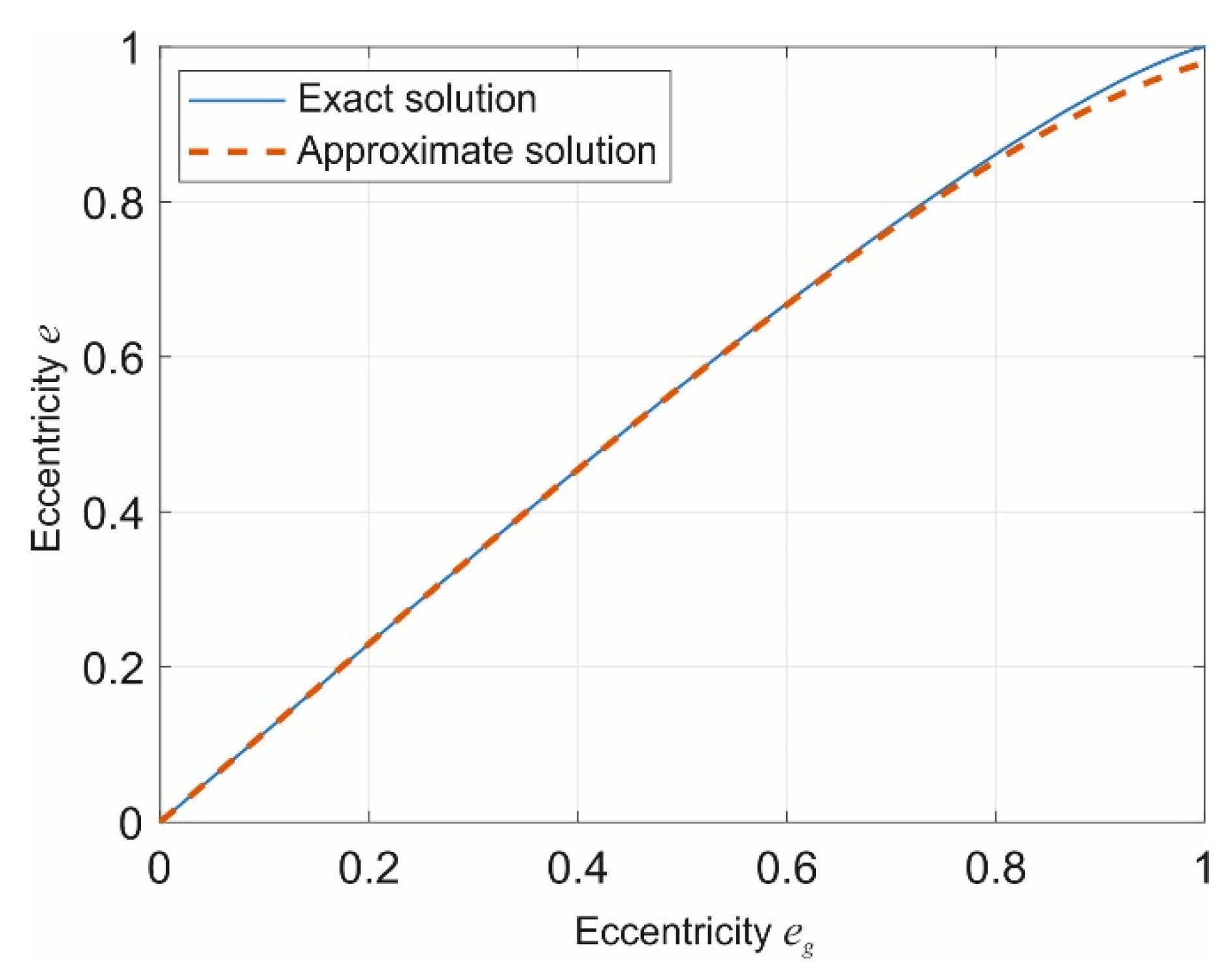
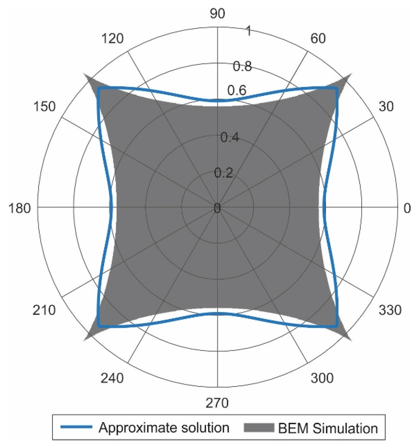
4.4. Contact of a Pyramid with Square Cross-Section

Let’s consider a linear profile

$$f(r,\phi )=r\tan \alpha \cos \phi ,-\frac{\pi }{4}<\phi <\frac{\pi }{4}$$

(57)

and similar equations for the angles $\pi /4<\phi <3\pi /4$, $3\pi /4<\phi <5\pi /4$ and $-3\pi /4<\phi <-\pi /4$, which describes a pyramid with square cross-sections and the angle $\alpha$ between the inclined planes of the pyramid and the horizon. In this case,

$$\psi (\phi )=\tan \alpha \cos \phi ,\overline{\psi }=\frac{2\sqrt{2}}{\pi }\tan \alpha$$

(58)

The boundary of the contact area is given by the relation (55) (see Figure 2)

$$a(\phi )=\frac{d}{\tan \alpha }\left(\frac{5}{2\sqrt{2}}-\frac{3\pi }{8}\cos \phi \right)\mathrm{for}-\frac{\pi }{4}<\phi <\frac{\pi }{4}\mathrm{usw}.$$

(59)

For the normal force, we get

$$F_N=\frac{2}{\pi }{E}^{*}\frac{d^2}{\overline{\psi }}=\frac{E^{*}{d}^2}{\sqrt{2}\tan \alpha }$$

(60)

Numerical simulation gives the solution $F_N=0.7395E^{*}{d}^2/\tan \alpha$ which is 4.6% larger than the above analytical result.

For the pressure distribution in the contact area, we obtain, according to (56),

$$p(r,\phi )=\frac{E^{*}}{2}\overline{\psi }\cdot \ln \left(\frac{a(\phi )}{r}+\sqrt{{\left(\frac{a(\phi )}{r}\right)}^2-1}\right)$$

(61)

4.5. Contact of Power-Law Shapes

Consider a profile having the form

$$f(r,\phi )=r^n\cdot \psi (\phi )$$

(62)

which means that all vertical cross-sections are self similar differing only by the scaling factor $\psi (\phi )$. The decomposition into a rotationally symmetric part and deviation is as follows

$$f_0(r)=r^n\cdot \overline{\psi },\delta f(r,\phi )=r^n\cdot \left(\psi (\phi )-\overline{\psi }\right)$$

(63)

where $\overline{\psi }$ is the average value of $\psi (\phi )$, Equation (34).

For all necessary auxiliary functions, we get

$$g_{\phi }(a)=\psi (\phi )\cdot \gamma (a),G_{\phi }(a)=\psi (\phi )\cdot \Upsilon (a),{\Upsilon }^{\prime }(a)=\gamma (a),g_0(a)=\overline{\psi }\cdot \gamma (a)$$

(64)

with

$$\gamma (a)=a{\displaystyle \underset{0}{\overset{a}{\int }}\frac{n{r}^{n-1}}{\sqrt{a^2-r^2}}\mathrm{d}r}={\kappa }_n{a}^n,{\kappa }_n={\displaystyle \underset{0}{\overset{1}{\int }}\frac{{\xi }^{n-1}\mathrm{d}\xi }{\sqrt{1-{\xi }^2}}}=\frac{\sqrt{\pi }}{2}\frac{n\mathsf{\Gamma }\left(\frac{n}{2}\right)}{\mathsf{\Gamma }\left(\frac{n}{2}+\frac{1}{2}\right)}$$

(65)

while $\mathsf{\Gamma }(\dots )$ is the gamma function.

For the deviations, we have

$$\delta g_{\phi }(a)={\kappa }_n{a}^n\left(\psi (\phi )-\overline{\psi }\right),\delta G_{\phi }(a)={\kappa }_n\frac{a^{n+1}}{n+1}\left(\psi (\phi )-\overline{\psi }\right)$$

(66)

The boundary of the contact area is given by the relation (28)

$$a(\phi )=a_0\left(1+\frac{n+2}{n(n+1)}\left(1-\frac{\psi (\phi )}{\overline{\psi }}\right)\right)$$

(67)

where $a_0$ is determined by the condition $\overline{\psi }{\kappa }_n{a}_0{}^n=d$:

$$a_0={\left(\frac{d}{{\kappa }_n\overline{\psi }}\right)}^{1/n}$$

(68)

The normal force is equal to

$$F_N(a_0)=2E^{*}{\displaystyle \underset{0}{\overset{a_0}{\int }}\left(d-\overline{\psi }{\kappa }_n{a}^n\right)}\mathrm{d}a=2E^{*}d{a}_0\frac{n}{n+1}=\frac{2n}{n+1}{E}^{*}{d}^{\frac{n+1}{n}}{\left({\kappa }_n\overline{\psi }\right)}^{-1/n}$$

(69)

The average pressure is equal to

$$\overline{p}=\frac{F_N(a_0)}{\pi a_0^2}=\frac{2n}{n+1}\frac{E^{*}{d}^{\frac{n-1}{n}}{\left({\kappa }_n\overline{\psi }\right)}^{1/n}}{\pi }$$

(70)

For the pressure distribution in the contact area, normalized by the average pressure, we obtain, according to (31),

$$p(r,\phi )=\frac{\left(n+1\right)}{2}{\displaystyle \underset{\overline{r}}{\overset{1}{\int }}\frac{{\xi }^{n-1}}{\sqrt{{\xi }^2-{\overline{r}}^2}}}\mathrm{d}\xi$$

(71)

with $\overline{r}=r/a(\phi )$. It is again the same result as that for an axisymmetric contact ([10], p. 78) with the substitution $r/a_0\to r/a(\phi )$.

5. Extended Method of Dimensionality Reduction (MDR) for Slightly Non-Axisymmetric Contacts

The above-sketched solution procedure can be considered as an extension of the Method of Dimensionality Reduction [11] to non-axisymmetric profiles. Let us summarize the above findings in the form of procedure that has to be applied for the solution of such problems.

We consider an “arbitrary” profile $z=f(r,\phi )$ underlying the following restrictions:

(1)

the profile deviates only weakly from an axisymmetric one;

(2)

during the normal indentation, only the normal contact force appears (no tilting forces or moments).

Under these conditions, the following procedure can be applied.

I.

In the first step, an “equivalent axisymmetric profile” is determined. In the first-order approximation, it was shown to be just the profile averaged over the angles:

$$f_0(r)=\frac{1}{2\pi }{\displaystyle \underset{0}{\overset{2\pi }{\int }}f(r,\phi )\mathrm{d}\phi }$$

(72)

II.

The profile can now be decomposed into an axisymmetric part and the small deviation

$$f(r,\phi )=f_0(r)+\delta f(r,\phi )$$

(73)

with

$$\delta f(r,\phi )=f(r,\phi )-f_0(r)$$

(74)

by definition.

III.

With the equivalent axisymmetric profile (72), the usual MDR solution procedure is applied. In particular, the MDR-transformed profile is determined as

$$g_0(a)=a{\displaystyle \underset{0}{\overset{a}{\int }}\frac{f_0{}^{\prime }\left(r\right)}{\sqrt{a^2-r^2}}\mathrm{d}r}$$

(75)

IV.

The effective radius $a_0$ is determined by the condition

$$d=g_0(a_0)$$

(76)

V.

The normal force is given by the equation

$$F_N=2E^{*}{\displaystyle \underset{0}{\overset{a_0}{\int }}\left(d-g_0(x)\right)\mathrm{d}x}$$

(77)

VI.

The effective pressure distribution in the contact area is given by the usual MDR equation [14] (p. 9)

$$p_0(r/a_0)=-\frac{1}{\pi }{\displaystyle \underset{r}{\overset{\infty }{\int }}\frac{q^{\prime }(x)}{\sqrt{x^2-r^2}}\mathrm{d}x}$$

(78)

with

$$q(x)=E^{*}\{\begin{array}{l}d-g(x),\left|x\right|<a_0\\ 0,\left|x\right|>a_0\end{array}$$

(79)

VII.

The true non-axisymmetric contact area is given by the equation

$$a(\phi )=a_0+\delta a(\phi )$$

(80)

where $\delta a(\phi )$ is determined by (28).

VIII.

Finally, the true pressure distribution is given by

$$p(r,\phi )=p_0(r/a(\phi ))$$

(81)

The last equation can be considered as a generalization of Fabrikant’s ansatz for flat-ended punches. Fabrikant states that the pressure distribution under a non-axisymmetric punch is equal to that under an axisymmetric punch but “rescaled” to the true shape of the contact area. Similarly, Equation (81) states that the contact pressure is equal to that under an “equivalent axisymmetric indenter” but rescaled to the true contact area. In the present paper, we have shown that Equation (81) is the exact first-order approximation for the power-law profiles (with arbitrary cross-section)—independently of the exponent of the power law. Even while it was not proven in a general case, the independence of the exponent gives hope that it could be a good approximation for arbitrarily shaped profiles. Testing of this hypothesis (e.g., through comparison with a numerical solution with BEM) is an important task of further studies.

6. Discussion

Using the Barber’s extremal principle, we derived explicit analytical relations for all essential contact properties of an indenter of “arbitrary” shape (under restriction that it should be close to an axisymmetric one). The solution provides the dependency of the normal force on the indentation depth, the size and the shape of the contact area, and the pressure distribution in the contact area. The derivation has been carried out under two assumptions (which are the main sources of deviation from the exact solution): (1) Fabrikant’s approximation for the stress of a flat-ended punch with arbitrary cross-section and (2) assumption of a small deviation of the indenter shape from an axial one. However, an acceptable accuracy is obtained even with relatively large deviations from axial symmetry, e.g., the eccentricity of the contact area for a paraboloid is given accurately up to an eccentricity of approximately 0.7. The deviation of normal force in a contact of a pyramid indenter with square cross-section is of about 4.6%. The whole calculation resembles the Method of Dimensionality Reduction very much and can be considered as its generalization for non-axially symmetric contacts. A central approximation used in this paper is Fabrikant’s approximation for the pressure under a flat punch. This approximation could be further improved by using higher-order corrections obtained by Golikova and Mossakovskii for the pressure distribution under plane stamps of nearly circular cross-section [15].

References

1. Hertz, H. Über die Berührung fester elastischer Körper. J. Für Die Reine Und Angew. Math. 1882, 92, 156–171. [Google Scholar] [CrossRef]
2. Popova, E.; Popov, V.L. Ludwig Föppl and Gerhard Schubert: Unknown classics of contact mechanics. ZAMM-J. Appl. Math. Mech./Z. Für Angew. Math. Und Mech. 2020, 100, e202000203. [Google Scholar] [CrossRef]
3. Föppl, L. Elastische Beanspruchung des Erdbodens unter Fundamenten. Forsch. Auf Dem Geb. Des Ing. A 1941, 12, 31–39. [Google Scholar] [CrossRef]
4. Schubert, G. Zur Frage der Druckverteilung unter elastisch gelagerten Tragwerken. Ing.-Arch. 1942, 13, 132–147. [Google Scholar] [CrossRef]
5. Barber, J.R.; Billings, D.A. An approximative solution for the contact area and elastic compliance of a smooth punch of arbitrary shape. Int. J. Mech. Sci. 1990, 32, 991–997. [Google Scholar] [CrossRef]
6. Shield, R.T. Load-displacement relations for elastic bodies. Z. Für Angew. Math. Und Phys. ZAMP 1967, 18, 682–693. [Google Scholar] [CrossRef]
7. Barber, J.R. Determining the contact area in elastic indentation problems. J. Strain Anal. 1974, 9, 230–232. [Google Scholar] [CrossRef]
8. Fabrikant, V.I. Flat punch of arbitrary shape on an elastic half-space. Int. J. Eng. Sci. 1986, 24, 1731–1740. [Google Scholar] [CrossRef]
9. Barber, J.R. Contact Mechanics; Springer: Cham, Switzerland, 2018; p. 585. [Google Scholar] [CrossRef]
10. Popov, V.L. Contact Mechanics and Friction. Physical Principles and Applications, 2nd ed.; Springer: Berlin/Heidelberg, Germany, 2017. [Google Scholar] [CrossRef]
11. Popov, V.L.; Heß, M. Method of Dimensionality Reduction in Contact Mechanics and Friction; Springer: Berlin/Heidelberg, Germany, 2015; 265p. [Google Scholar] [CrossRef]
12. Li, Q.; Technische Universität, Berlin, Germany. Personal Communication, 2022.
13. Pohrt, R.; Li, Q. Complete boundary element formulation for normal and tangential contact problems. Phys. Mesomech. 2014, 17, 334–340. [Google Scholar] [CrossRef]
14. Popov, V.L.; Heß, M.; Willert, E. Handbook of Contact Mechanics. Exact Solutions of Axisymmetric Contact Problems; Springer: Berlin/Heidelberg, Germany, 2019. [Google Scholar] [CrossRef]
15. Golikova, S.S.; Mossakovskii, V.I. Pressure of a plane stamp of nearly circular cross section on an elastic half-space. PMM J. Appl. Math. Mech. 1976, 40, 1085–1088. [Google Scholar] [CrossRef]
Figure 1. Eccentricity e of the contact area as a function of eg according to Equation (49) (dashed line) and comparison with the value according to the Hertzian solution [9] (solid line).
Symmetry 14 00390 g001
Figure 2. The normalized contact boundary line ( a ( φ ) tan α / d ) according to Equation (59) (blue line) and the result of numerical simulation with Boundary Element Method (gray figure). Numerical data have been obtained by Qiang Li [12] with the method described in [13].
Symmetry 14 00390 g002
Publisher’s Note: MDPI stays neutral with regard to jurisdictional claims in published maps and institutional affiliations.