

Autonomous Navigation and Obstacle Avoidance for Small VTOL UAV in Unknown Environments


Abstract
1. Introduction
1.1. Autonomous Positioning
1.2. Map Building and Trajectory Planning
1.3. Target Detection and Recognition
2. Autonomous Positioning
2.1. The Introduction of the Autonomous Positioning Module
2.2. The Preprocessing of Signals
2.2.1. Visual Front-End
- (1)
- Bidirectional Kanade–Lucas–Tomasi (KLT) tracking
- (2)
- The selection strategy of the key frames
2.2.2. IMU Pre-Integration
2.3. Pose Initialization
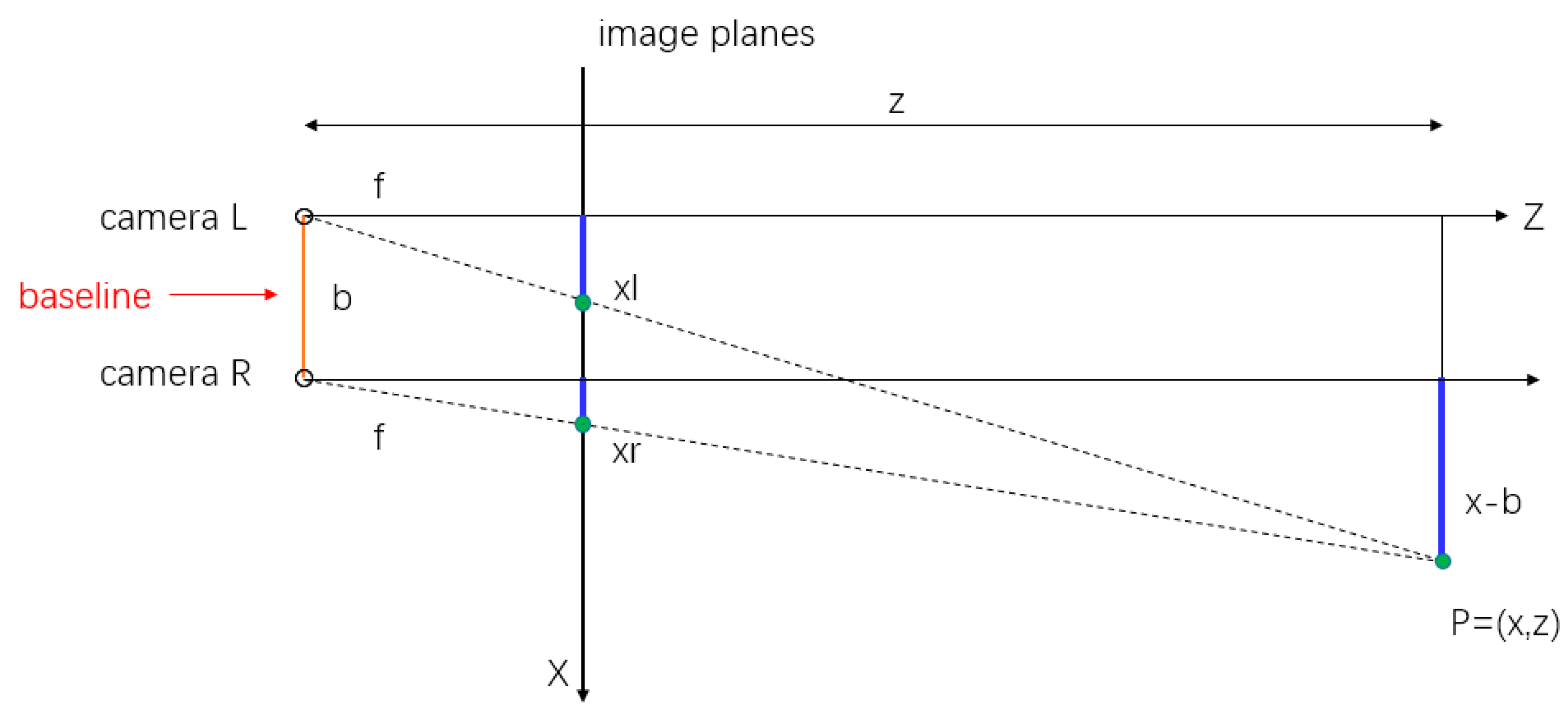
2.3.1. The Depth Estimation of Feature Points
2.3.2. Pose Initialization
2.4. VIO Algorithm
2.4.1. Sliding Window Method
2.4.2. The Calculation of IMU Measurement Residual
2.4.3. Visual Measurement Residual
2.5. Loopback Optimization
2.5.1. DBoW Loopback Detection
2.5.2. Bidirectional KLT Tracking and PNP Relocation
2.5.3. The Management of 4-Dof Pose Diagram
2.6. Simulation Analysis Test
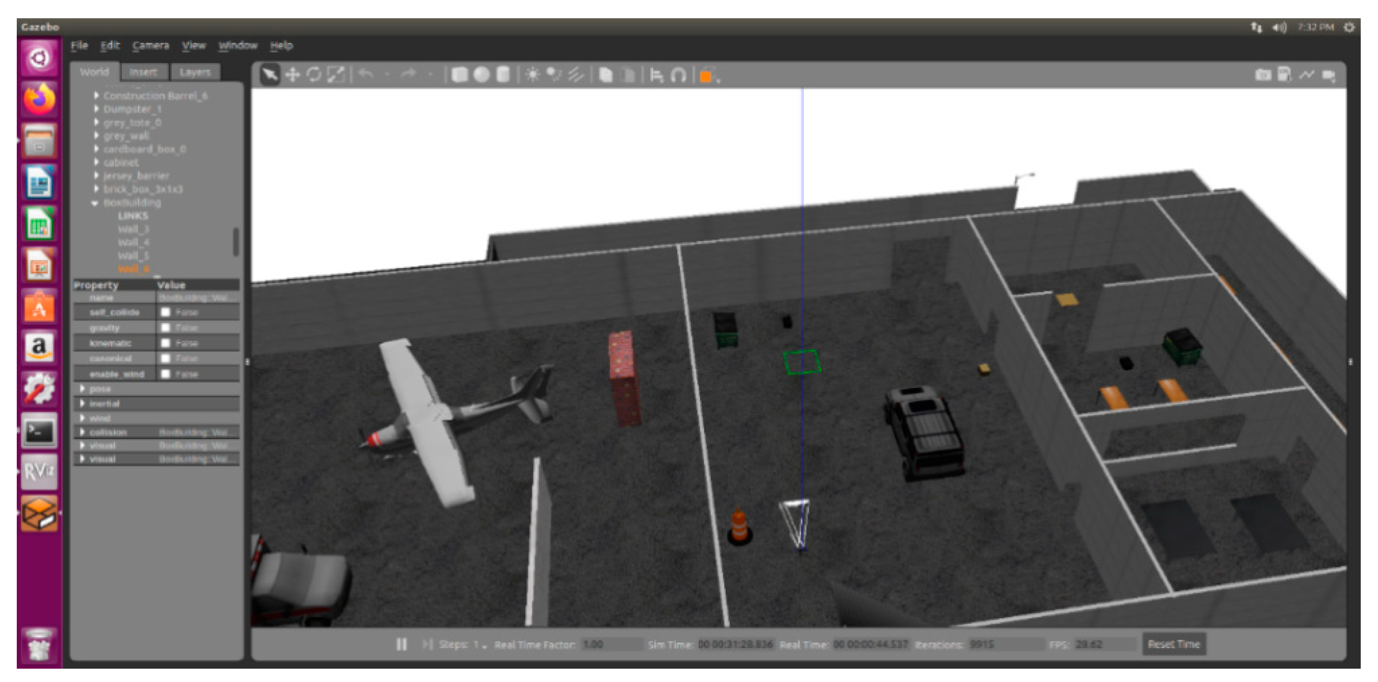
2.6.1. Simulation Engine Gazebo
- To test a robot algorithm;
- To design a robot;
- To perform a regression test in actual scenarios.
- It contains multiple physics engines;
- It contains a rich library of robot models and environments;
- It contains a variety of sensors;
- The program is convenient to design and has a simple graphical interface.
2.6.2. Simulation System


| Maximum error along X direction | Yaw angle error | ||
| Maximum error along Y direction | Absolute error | ||
| Maximum error along Z direction | Calculated closed-loop error | ||
| Standard deviation | X | ||
| Y | |||
| Z | |||
2.7. Section Conclusion
3. Detailed Design of the Map-Building and Trajectory-Planning Algorithm
3.1. The Introduction of the Autonomous Positioning Module
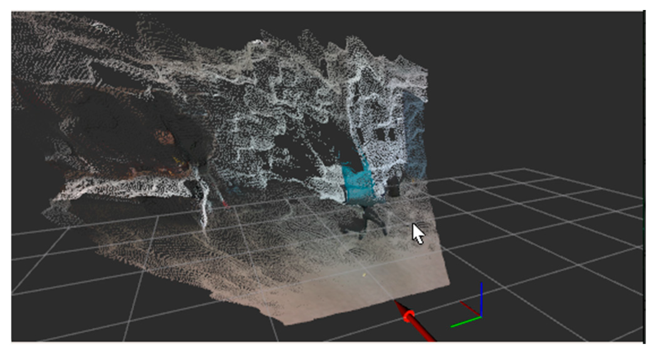
3.2. Octree Map
- It has a huge amount of data, and there is serious redundant storage and information redundancy.
- Point cloud maps are stored in continuous space, which means they can’t be directly discretized and fast searched.
- This method cannot deal with moving objects and observation errors because we can add objects into the maps but not remove objects from maps.
3.2.1. The Data Structure of the Octree Map
3.2.2. Node Probability Updating
3.3. Path Planning
3.3.1. Basic RRT Algorithm
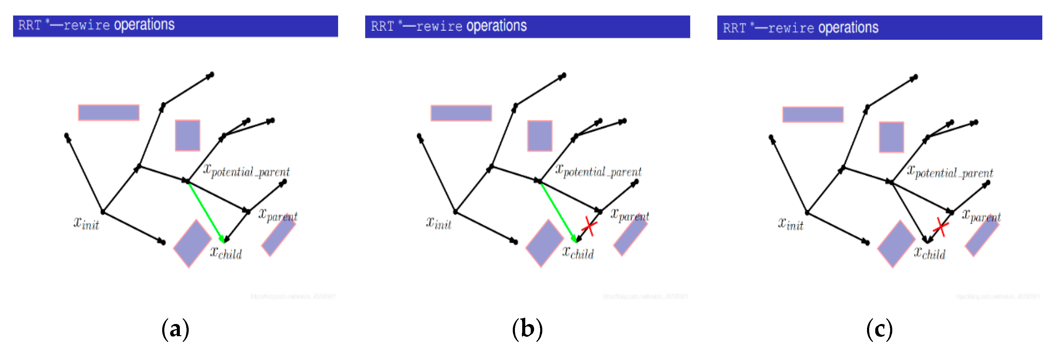
3.3.2. RRT* Algorithm
- (1)
- Generate a random point Xrand;
- (2)
- Find the nearest node Xnearest from Xrand on the tree;
- (3)
- Connect Xrand with Xnearest;
- (4)
- With Xrand as the center, search for nodes in the tree with a certain radius and find out the set of potential parent nodes {Xpotential_parent}. The purpose is to update Xrand and observe whether there is a better parent node;
- (5)
- Start with a potential parent, Xpotential_parent;
- (6)
- Calculate the cost of Xnearest being the parent node;
- (7)
- Instead of performing collision detection, connect Xpotential_parent with Xchild (that is, Xrand) and calculate the path cost;
- (8)
- Compare the cost of the new path with that of the initial path. If the cost of the new path is smaller, the collision detection will be carried out; otherwise, the next potential parent node will be replaced;
- (9)
- If collision detection fails, the potential parent node will not act as the new parent node;
- (10)
- Turn to the next potential parent;
- (11)
- Connect the potential parent node to Xchild (that is, Xrand) and calculate the path cost;
- (12)
- Compare the cost of the new path with the cost of the original path. If the cost of the new path is smaller, the collision detection will be carried out; if the cost of the new path is larger, the next potential parent node will be replaced;
- (13)
- The collision detection passes;
- (14)
- Delete the previous edges from the tree;
- (15)
- Add a new edge to the tree, and take the current Xpotential_parent as the parent of Xrand.


3.4. Smoothing the Interpolation of Third-Order β Spline
3.4.1. Node Table
3.4.2. Basic Function Tables
3.4.3. Calculation
3.5. Simulation Test and Analysis
3.6. Section Conclusion
4. The Detailed Design of the Target Detection and Recognition Algorithm
4.1. The Introduction of Target Detection and Recognition Module
4.2. Target Detection Network
- (1)
- Features extraction network
- (2)
- Residual mechanism
- (3)
- Feature map
4.3. TensorRT Inference Acceleration
- (1)
- Interlayer fusion and tensor fusion
- (2)
- Data accuracy calibration
- (3)
- CUDA core optimization
- (4)
- Tensor memory management
- (5)
- GPU multi-stream optimization
4.4. Analysis Test
4.5. Section Conclusion
5. Technical Validation
5.1. Introduction of the Platform Plan
5.1.1. The Fuselage Part
- (1)
- Power system
- (2)
- Frame design
- (3)
- Battery
- (4)
- Flight control system

5.1.2. Autonomous Navigation System
- (1)
- Core processing unit
- (2)
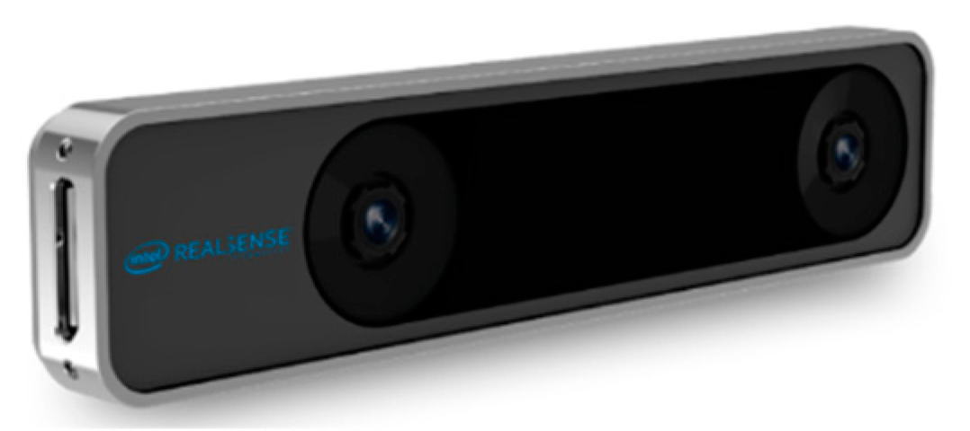
- Sensor
5.1.3. Data Transfer System
5.1.4. Ground Control System
5.2. Flight Test
5.2.1. Performance Test
- (1)
- Positioning accuracy of integrated navigation
- Combined navigation and positioning accuracy (CEP): ≤0.2 m;
- Fixed-altitude, fixed-point flight accuracy (CEP): ≤0.5 m (RMS).
- (2)
- (3)
- Obstacle detection channel and range
- (4)
- Minimum size of detectable obstacle
- (5)
- Obstacle detection rate
5.2.2. Single-Machine Indoor Autonomous Obstacle Avoidance and Navigation
- (1)
- Scene experiment with three obstacles
- (2)
- Scene experiment with two obstacles
6. Conclusions
- ⮚
- Advantages: (1) Uses distributed hardware solution to realize obstacle observation (D435i) and SLAM (T265) functions, which greatly reduces the computational power requirements of the airborne computer; (2) optimizes the YOLO network using TensorRT so it can run in real time on the onboard computer; (3) OCtomAP mapping, RRT* and β spline curve fitting are finished mainly by CPU, target recognition mainly by GPU, making full use of onboard computer resources.
- ⮚
- Weaknesses: (1) The basic assumption of a l-SLAM system is that the environment remains static. If the environment moves in whole or part, the localization results will be disturbed; (2) OctomAP requires a cumulative period of stable observations to effectively identify obstacles, which makes the UAV unable to effectively respond to obstacles that suddenly appear; (3) the motion trajectory generated by 3-RRT* and β spline curve only has position command, but no speed and acceleration command, and so cannot guide the UAV to fly at high speed.
Author Contributions
Funding
Data Availability Statement
Conflicts of Interest
Nomenclature
| UAV | Unmanned aerial vehicle |
| GNSS | Global navigation satellite system |
| SLAM | Simultaneous location and mapping |
| USV | Unmanned surface vehicle |
| UAM | Urban air mobility |
| SAFDAN | Solar atomic frequency discriminator for autonomous navigation |
| VPC | Visual predictive control |
| MPC | Model predictive control |
| UUV | Unmanned underwater vehicle |
| VR | Virtual reality |
| GPS | Global positioning system |
| VI-SLAM | Visual–inertial simultaneous localization and mapping |
| IMU | Inertial measurement unit |
| VIO | Visual–inertial odometry |
| KLT tracking | Kanade–Lucas–Tomasi tracking |
| RRT | Rapidly exploring random trees |
| CNN | Convolutional neural network |
| RCNN | Region-convolutional neural network |
| SSD | Single shot multi-box detector |
| VGG | Visual geometry group |
| FPN | Feature pyramid network |
| GPU | Graphics processing unit |
| GIE | GPU inference engine |
| CUDA | Compute unified device architecture |
| CBR | Case-based reasoning |
| FP32 | Full 32-bit precision |
| FOV | Field of view |
References
- Li, Z.; Lu, Y.; Shi, Y.; Wang, Z.; Qiao, W.; Liu, Y. A Dyna-Q-based solution for UAV networks against smart jamming attacks. Symmetry 2019, 11, 617. [Google Scholar] [CrossRef]
- Kuriki, Y.; Namerikawa, T. Consensus-based cooperative formation control with collision avoidance for a multi-UAV system. In Proceedings of the 2014 American Control Conference, Portland, OR, USA, 4–6 June 2014; IEEE: New York, NY, USA, 2014; pp. 2077–2082. [Google Scholar]
- Kwak, J.; Park, J.H.; Sung, Y. Unmanned aerial vehicle flight point classification algorithm based on symmetric big data. Symmetry 2016, 9, 1. [Google Scholar] [CrossRef]
- Turan, E.; Speretta, S.; Gill, E. Autonomous navigation for deep space small satellites: Scientific and technological advances. Acta Astronaut. 2022, 193, 56–74. [Google Scholar] [CrossRef]
- Kayhani, N.; Zhao, W.; McCabe, B.; Schoellig, A.P. Tag-based visual-inertial localization of unmanned aerial vehicles in indoor construction environments using an on-manifold extended Kalman filter. Autom. Constr. 2022, 135, 104112. [Google Scholar] [CrossRef]
- Li, Z.; Zhang, Y. Constrained ESKF for UAV Positioning in Indoor Corridor Environment Based on IMU and WiFi. Sensors 2022, 22, 391. [Google Scholar] [CrossRef]
- Aldao, E.; González-de Santos, L.M.; González-Jorge, H. LiDAR Based Detect and Avoid System for UAV Navigation in UAM Corridors. Drones 2022, 6, 185. [Google Scholar] [CrossRef]
- Zhang, W.; Yang, Y.; You, W.; Zheng, J.; Ye, H.; Ji, K.; Chen, X.; Lin, X.; Huang, Q.; Cheng, X.; et al. Autonomous navigation method and technology implementation of high-precision solar spectral velocity measurement. Sci. China Phys. Mech. Astron. 2022, 65, 289606. [Google Scholar] [CrossRef]
- Ramezani Dooraki, A.; Lee, D.J. A Multi-Objective Reinforcement Learning Based Controller for Autonomous Navigation in Challenging Environments. Machines 2022, 10, 500. [Google Scholar] [CrossRef]
- Durand Petiteville, A.; Cadenat, V. Advanced Visual Predictive Control Scheme for the Navigation Problem. J. Intell. Robot. Syst. 2022, 105, 35. [Google Scholar] [CrossRef]
- Specht, C.; Świtalski, E.; Specht, M. Application of an autonomous/unmanned survey vessel (ASV/USV) in bathymetric measurements. Pol. Marit. Res. 2017, nr 3, 36–44. [Google Scholar] [CrossRef]
- Xie, S.; Wu, P.; Peng, Y.; Luo, J.; Qu, D.; Li, Q.; Gu, J. The obstacle avoidance planning of USV based on improved artificial potential field. In Proceedings of the 2014 IEEE International Conference on Information and Automation (ICIA), Hailar, China, 28–30 July 2014; IEEE: New York, NY, USA, 2014; pp. 746–751. [Google Scholar]
- Wang, X.; Yadav, V.; Balakrishnan, S.N. Cooperative UAV formation flying with obstacle/collision avoidance. IEEE Trans. Control. Syst. Technol. 2007, 15, 672–679. [Google Scholar] [CrossRef]
- Manhães, M.M.M.; Scherer, S.A.; Voss, M.; Douat, L.R.; Rauschenbach, T. UUV Simulator: A Gazebo-based package for underwater intervention and multi-robot simulation. In Proceedings of the OCEANS 2016 MTS/IEEE Monterey, Monterey, CA, USA, 19–23 September 2016; pp. 1–8. [Google Scholar]
- Liu, L.; Wu, Y.; Fu, G.; Zhou, C. An Improved Four-Rotor UAV Autonomous Navigation Multisensor Fusion Depth Learning. Wirel. Commun. Mob. Comput. 2022, 2022, 2701359. [Google Scholar] [CrossRef]
- Sajjadi, S.; Mehrandezh, M.; Janabi-Sharifi, F. A Cascaded and Adaptive Visual Predictive Control Approach for Real-Time Dynamic Visual Servoing. Drones 2022, 6, 127. [Google Scholar] [CrossRef]
- Nascimento, T.; Saska, M. Embedded Fast Nonlinear Model Predictive Control for Micro Aerial Vehicles. J. Intell. Robot. Syst. 2021, 103, 74. [Google Scholar] [CrossRef]
- Ambroziak, L.; Ciężkowski, M.; Wolniakowski, A.; Romaniuk, S.; Bożko, A.; Ołdziej, D.; Kownacki, C. Experimental tests of hybrid VTOL unmanned aerial vehicle designed for surveillance missions and operations in maritime conditions from ship-based helipads. J. Field Robot. 2021, 39, 203–217. [Google Scholar] [CrossRef]
- Hassan, S.A.; Rahim, T.; Shin, S.Y. An Improved Deep Convolutional Neural Network-Based Autonomous Road Inspection Scheme Using Unmanned Aerial Vehicles. Electronics 2021, 10, 2764. [Google Scholar] [CrossRef]
- Zhu, H.; Liu, C.; Li, M.; Shang, B.; Liu, M. Unmanned aerial vehicle passive detection for Internet of Space Things. Phys. Commun. 2021, 49, 101474. [Google Scholar] [CrossRef]
- He, L.; Aouf, N.; Song, B. Explainable Deep Reinforcement Learning for UAV autonomous path planning. Aerosp. Sci. Technol. 2021, 118, 107052. [Google Scholar] [CrossRef]
- Miranda, V.R.; Rezende, A.; Rocha, T.L.; Azpúrua, H.; Pimenta, L.C.; Freitas, G.M. Autonomous Navigation System for a Delivery Drone. J. Control. Autom. Electr. Syst. 2022, 33, 141–155. [Google Scholar] [CrossRef]
- Zhao, X.; Chong, J.; Qi, X.; Yang, Z. Vision Object-Oriented Augmented Sampling-Based Autonomous Navigation for Micro Aerial Vehicles. Drones 2021, 5, 107. [Google Scholar] [CrossRef]
- Ren, Y.; Liu, X.; Liu, W. DBCAMM: A novel density based clustering algorithm via using the Mahalanobis metric. Appl. Soft Comput. 2012, 12, 1542–1554. [Google Scholar] [CrossRef]
- Guitton, A.; Symes, W.W. Robust inversion of seismic data using the Huber norm. Geophysics 2003, 68, 1310–1319. [Google Scholar] [CrossRef]
- Elmokadem, T.; Savkin, A.V. Towards Fully Autonomous UAVs: A Survey. Sensors 2021, 21, 6223. [Google Scholar] [CrossRef] [PubMed]
- Zammit, C.; Van Kampen, E.J. Comparison between A* and RRT algorithms for UAV path planning. In Proceedings of the 2018 AIAA Guidance Navigation, and Control Conference, Kissimmee, FL, USA, 8–12 January 2018; p. 1846. [Google Scholar]
- Aguilar, W.G.; Morales, S.; Ruiz, H.; Abad, V. RRT* GL based optimal path planning for real-time navigation of UAVs. In Proceedings of the International Work-Conference on Artificial Neural Networks, Cádiz, Spain, 14–16 June 2017; Springer: Cham, Switzerland, 2017; pp. 585–595. [Google Scholar]
- Wang, C.; Meng, M.Q.H. Variant step size RRT: An efficient path planner for UAV in complex environments. In Proceedings of the 2016 IEEE International Conference on Real-Time Computing and Robotics (RCAR), Angkor Wat, Cambodia, 6–10 June 2016; IEEE: New York, NY, USA, 2016; pp. 555–560. [Google Scholar]
- Kang, Z.; Zou, W. Improving accuracy of VI-SLAM with fish-eye camera based on biases of map points. Adv. Robot. 2020, 34, 1272–1278. [Google Scholar] [CrossRef]


| Ability | 10 W Mode | 15 W Mode |
|---|---|---|
| AI performance | 14 TOPS (INT8) | 21 TOPS (INT8) |
| GPU | 384-core NVIDIA Volta™ GPU with 48 Tensor cores | |
| GPU max freq | 800 MHz | 1100 MHz |
| CPU | 6-core NVIDIA Carmel ARM®v8.2 64-bit CPU 6 MB L2 + 4 MB L3 | |
| CPU max freq | 2-core @ 1500 MHz 4-core @ 1200 MHz | 2-core @ 1900 MHz 4/6-core @ 1400 Mhz |
| Memory | 8 GB 128-bit LPDDR4x @ 1600 MHz 51.2 GB/s | |
| Storage | 16 GB eMMC 5.1 | |
| Power | 10 W|15 W | |
| Computing Platforms | Initialization/ms | Average Time/ms |
|---|---|---|
| CUP | - | 790 |
| GPU(CUDA) | 2310 | 85 |
| GPU(TensorRT) | 1103 | 12 |
| Model | AP6750-10T |
| Type | Distributed wireless router |
| Wireless standard | IEEE 802.11 a/b/g/ac/ac wave2, support 2×2MIMO |
| Wireless rate | 3000 Mbps |
| Working frequency range | 2.4 GHz, 5 GHz |
| Support agreement | 802.11a/b/g/n/ac/ax |
| Software parameters | |
| WPS support | Supports WPS one-click encryption |
| Safety performance | Support Open System authentication Support WEP authentication, and support 64-bit, 128-bit, 152-bit, and 192-bit encryption bytes Support wap2-psk Support wpa2-802.1x Support wpa3-sae Support wap3-802.1x Support wap-wpa2 Support wap-wpa3 |
| Internet management | Support IEEE 802.3ab standard Support sub-negotiation of rate and duplex mode Compatible with the IEEE 802.1 q Support NAT |
| Qos support | Based on the WMM, it supports the WMM power saving mode, uplink packet priority mapping, queue mapping, queue mapping, VR/ mobile game application acceleration, and hierarchical HQos scheduling for airports. |
| Hardware parameters | |
| Local network interfaces | 2 × 10 GE electrical interface, 1 × 10 GE SFP+ |
| Other interfaces | one |
| Type of antenna | Built-in type |
| Working environment | Temperature: −10~+50 °C |
Publisher’s Note: MDPI stays neutral with regard to jurisdictional claims in published maps and institutional affiliations. |
© 2022 by the authors. Licensee MDPI, Basel, Switzerland. This article is an open access article distributed under the terms and conditions of the Creative Commons Attribution (CC BY) license (https://creativecommons.org/licenses/by/4.0/).
Share and Cite
Chen, C.; Wang, Z.; Gong, Z.; Cai, P.; Zhang, C.; Li, Y. Autonomous Navigation and Obstacle Avoidance for Small VTOL UAV in Unknown Environments. Symmetry 2022, 14, 2608. https://doi.org/10.3390/sym14122608
Chen C, Wang Z, Gong Z, Cai P, Zhang C, Li Y. Autonomous Navigation and Obstacle Avoidance for Small VTOL UAV in Unknown Environments. Symmetry. 2022; 14(12):2608. https://doi.org/10.3390/sym14122608
Chicago/Turabian StyleChen, Cheng, Zian Wang, Zheng Gong, Pengcheng Cai, Chengxi Zhang, and Yi Li. 2022. "Autonomous Navigation and Obstacle Avoidance for Small VTOL UAV in Unknown Environments" Symmetry 14, no. 12: 2608. https://doi.org/10.3390/sym14122608
APA StyleChen, C., Wang, Z., Gong, Z., Cai, P., Zhang, C., & Li, Y. (2022). Autonomous Navigation and Obstacle Avoidance for Small VTOL UAV in Unknown Environments. Symmetry, 14(12), 2608. https://doi.org/10.3390/sym14122608