Abstract
This paper presents a novel algorithm about the industrial robot contouring control based on the NURBS (non-uniform rational B-spline) curve. First, aiming at the error between the industrial robot’s actual trajectory and the desired trajectory, the contour error is proposed as the trajectory evaluation index, and the estimation algorithm of contour error based on the tangent approximation is proposed. Based on the tangent approximation algorithm, the estimation algorithm of contour error in the local task coordinate frame is proposed to realize the transformation from the Cartesian coordinate frame to the local task coordinate frame. Second, according to the configuration of the industrial robot, a modified cross-coupling control scheme based on the local task coordinate frame is designed. Finally, the Bernoulli’s lemniscate curves are constructed by NURBS curve and five-order polynomial curve, respectively, and they are symmetrical. The contrast experiment is designed using the two types of constructed Bernoulli’s lemniscate curves as the incentive trajectory. Through the analysis and comparison between the obtained uniaxial tracking error and the contour error curve of the two incentive trajectories, it is concluded that the incentive trajectory constructed by the NURBS curve has better contour control performance than that constructed by the five-order polynomial curve. The results drawn from this paper lay a certain foundation for the future high-precision contouring control of industrial robots.
1. Introduction
In the working process of the industrial robot, the quality of trajectory makes a difference in the overall working process of the robot [1]. Generally speaking, for the industrial robot, given all the critical path points through online-teaching, there exists trajectory error between the actual trajectory and the desired trajectory inevitably because the dynamic response process of the robot always lags behind the reference input [2,3,4], which are mainly manifested in tracking error and contour error [5,6]. With multi-joint motors of the robot coordinate with each other, the tracking error of single axis motor will superimpose on the operation trajectory, which forms contour errors [7]. Tracking error could be defined as the distance between the desired position and the actual position at a certain moment, while the definition of the contour error is the tangential distance between the actual position at a certain moment and the desired track point. That is to say, contour error could also be defined as the distance between the desired trajectory and the actual trajectory [8]. According to the definition of tracking error and contour error, tracking error describes the distance between two different points, while contour error describes the distance from the actual point to a set of points. In the research of the precision contour error control, the value of contour error is less than or equal to the tracking error’s value, and the tracking error could be regarded as the maximum value of e contour error at the very moment. However, the tracking error and contour error does not have a specific relation with each other, and according to the two definitions above, the two kinds of error is completely different [9]. The contour error and tracking error of the robot operation trajectory are shown in Figure 1.
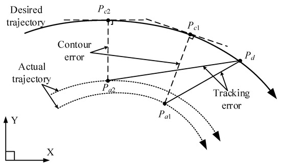
Figure 1.
Contour error and tracking error.
In order to explain the difference between the contour error and the tracking error more directly, as shown in Figure 1, is the expected point, while point and are the actual points at different moments. Then, the tracking error corresponding to the actual point and could be expressed as and , meanwhile and are the contour error corresponding to the actual point and . It could be seen from Figure 1 that the tracking error is less than , but the contour error is greater than . When , , the opposite is not true. It is obviously concluded that has more practical significance for the contour control than . According to the above definitions, it is easy to conclude that the contour error only depends on the current actual position and the geometry shape of the desired trajectory, and is irrelevant to the desired point and the tracking error.
The calculation of the contour error depends on the shape of the robot’s end-effector trajectory. Contour error could be accurately calculated when the trajectory is a simple curve such as a straight line or arc [10,11]. However, under any common smooth curve, contour error could not be accurately calculated [12], which could be approximated with a variety of approximation algorithms in these cases. Yeh [13] et al. proposed a general curve contour error estimation algorithm based on the tangent approximation of the line contour error, which achieved good estimation effect for curves with small curvature. J. Yang [14] et al. improved the estimation accuracy of the contour error through the osculating circle at any point of the curve as an approximation condition. Y. Zhu [15] et al. proposed new contour error calculation model under task coordinates, and calculated the first order approximation of the contour error, which does not depend on the single axis tracking error. During the calculation process, we just need to know the equation of the desired trajectory, and the coordinates of the actual point, which achieved good results in planar curve contour error calculation. However, the contour error calculation for the spatial curve needs further research [16]. In addition, with the improvement of the processor’s computing speed in robot system, F. Huo [17] took the minimum value of the distance between the actual position points and a series of the path points on the desired trajectory as the estimated value of the contour error. When the interpolation period is short, the estimation effect of this algorithm is better for the contour error, but this kind of algorithm needs higher controller performance.
In order to reduce contour error, and improve trajectory performance, L.B [18] et al. applied the single-axis uncoupled control algorithm to control a single axis separately, which reduced the tracking error of each axis and improved track accuracy. Jin.Z [19] established contour error models of the OMPR in straight line, arc, and spiral trajectories are. Then, they established feed-forward combined multi-axis cross-coupled contour control compensation strategy which achieved good control effect. L. Wang [20] et al. designed a cross-coupled controller in which the inputs of the controller were the tracking errors obtained according to the five feed-axes commands and encoder feedbacks. S. Wang [21] et al. designed a self-adaptive fuzzy PID cross-coupled controller which can eliminate the influence of the characteristics mismatching and parameter difference of each axis. N.T. Hu [22] et al. proposed a new structure of cross-coupled position command shaping controller using control scheme for the precise tracking in the multiaxial motion control which remarkably reduces contour error. Cross coupling control was applied to solve the multi-axis motion incoordination caused by a large tracking error of single axis which achieved good control effect for the motion platform with orthogonal axes, and multi-axis CNC machining platform [10,19,20,23,24,25].
However, most of the estimation algorithms mentioned above for the contour error are suitable for the contour error of the planar curve; furthermore, the estimation algorithms for the spatial curve contour error are rarely involved. In recent years, more and more researchers have started to engage in this field. H. Zhao [4] et al. proposed a components-based contouring control structure for a six-degree of freedom robot. A locally iterative robotic contour error estimation approach with high accuracy and high efficiency was designed by compensating the weighted contour error components to the velocity commands in the robotic task space. Z. Wang [26] et al. proposed an Atiken method based on acceleration iterative to achieve higher estimation accuracy of contouring error and reduce the real-time calculation burden, and verified the effectiveness of the proposed method through experiments. The estimation algorithms mentioned above are mostly used in CNC machining platforms with orthogonal axes, and the control algorithm design of the spatial curve contour error is also mostly based on the above platforms [27].
Compared with the CNC machine platform, industrial robot has higher degrees of freedom and more complex actions. Therefore, it is necessary to design a contour error control algorithm which suits the robot contour control [28,29,30]. According to the configuration of the industrial robot, this paper presents a trajectory planning algorithm in the Cartesian space based on the NURBS curve [31,32,33]. NURBS curve is often used in robot path generation algorithms. Compared with other algorithms, the NURBS algorithm is more conducive to the generation and processing of multidimensional and irregular curves. G. Wu [34] et al. proposed a path planning method based on the NURBS curve with optimal robot performance. By solving a multi-objective optimization problem, the optimal curve parameters and the execution time distributed along the curve segments can be obtained simultaneously. K. Erwinski [35] et al. presented a NURBS toolpath federate profile generation algorithm for a biaxial linear motor control system, and constructed two-dimensional plane curves of “Bird” and “flower” by using NURBS toolpath with marked control points and polygons. On the basis of existing research results, this paper presents an approximation algorithm to approximate the contour error of the robot, and constructs the incentive trajectory by the NURBS curve. Then, based on the approximation algorithm, a modified cross-coupling controller in the local task coordinate frame is presented, which realizes the contour control of the robot, improves the trajectory performance and quality of industrial robot’s working process.
The main contributions of this paper could be summarized as follows:
- (1)
- A contour error approximation algorithm for the spatial curve based on under the local task coordinate frame was proposed, and realizes the transformation from the tracking error of each axis on the desired trajectory to the contour error;
- (2)
- A modified cross-coupling control algorithm is proposed which realizes the error feedback control from the tracking error to the contour error.
- (3)
- The evaluation system of contour error controller with root mean square as evaluation index is established, and Bernoulli’s lemniscate curves as the incentive trajectory was constructed by NURBS curve through adjusting its parameters.
This paper is organized as follows. In Section 2, the contour error approximation algorithm of general spatial curve in the local task coordinate frame is proposed. In Section 3, based on the above contour error approximation algorithm, a modified cross-coupling control algorithm is proposed, which is suitable for the industrial robot configuration. In Section 4, based on the improved cross-coupling control algorithm, the NURBS curve trajectory planning algorithm is compared with the five-order polynomial planning algorithm, and illustrates the effectiveness of the NURBS planning and modified cross-coupling controller. In Section 5, this paper arrives at some conclusions.
2. Contour Error Estimation Algorithm
2.1. Contour Error Estimation Based on Tangent Approximation
As shown in Figure 2, the contour error of a line can be accurately calculated. Given the actual point , expected trajectory point , then tracking error could be defined as . Given direction vector of the planar line , and is the included angle between the vector and , . Then the contour error of the planar line could be expressed as,
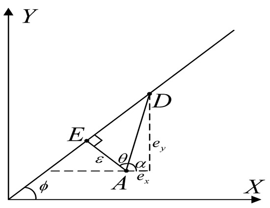
Figure 2.
The contour error of a planar line.
Similarly, for a line in the Cartesian space, its parametric equation is shown as,
Then, the contour error of a spatial straight line can also be expressed in the form of Equation (1). In addition, a spatial straight line could be regarded as the intersection of two planes, i.e.,
where , are the normal vectors of the two planes shown in Equation (3). Then the direction vector of the spatial line is,
For common curves, it is difficult to obtain the geometric description of the desired trajectory, thus it is difficult to calculate the contour error of the common curves. However, the calculation of the contour error about a common curve can be simplified as the tangency distance between the actual point and the corresponding desired point, as shown in Figure 3.
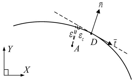
Figure 3.
Contour error estimation based on tangential approximation.
In Figure 3, contour error could be approximated by which is the distance of the tangent line from point to point , and is the unit tangent vector at point , is the unit normal vector, then,
The parametric equation of the spatial curves could be expressed as,
Tangent vector at any point of the spatial curve is . Thus,
In addition, a spatial curve can be thought as the intersection of surfaces, i.e.,
where , are the normal vectors of the two surfaces shown in Equation (8). Then the tangent vector of the common spatial curve is,
2.2. Contour Error in Local Task Coordinate Frame
In Figure 3, and are orthogonal to each other at point on the desired trajectory, where is the unit tangent vector, and is the unit normal vector, which constitute the local task coordinate frame at point . From Cartesian coordinates to the local task coordinates, we have the following transformation of the coordinates,
where T is the transformation matrix from the Cartesian coordinate frame to the local task coordinate frame, and,
In addition, Equation (10) is equivalent to the Equation (1). For the common curves, the approximate value of the tangent approximation could be used to estimate the actual contour error.
For common planar curve whose parametric equation is,
and the unit tangent vector is,
the unit normal vector is,
then,
where Equation (10) is equivalent to Equation (15).
The above is the case of a planar curve. In the case of the spatial curve, the Frenet local task coordinate frame as shown in Figure 4 can be established at point ,
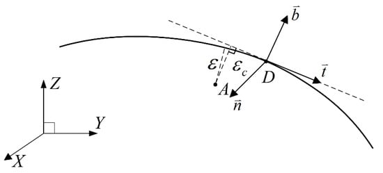
Figure 4.
Frenet local task coordinate frame of spatial curve.
Similar with the case of a planar curve, is the unit tangent vector, is the unit principal normal vector, is the unit binormal vector, furthermore, , , are orthogonal to each other, and satisfy the right-hand coordinate frame. Vector and form the osculating plane at point , and form the rectifying plane, and form the normal plane.
Referring to Equation (6) for parametric equation of spatial curve, then,
and,
The equations of normal plane , osculating plane , and rectifying plane at point are:
The estimated value of the contour error at point can be decomposed into the distance from point to the osculating plane , and the distance from point to the rectifying plane , which could be expressed in the form of:
i.e.,
where the first, second, and third lines of are the , , and components of , , and respectively, referring to Equations (16)–(18). Obviously, Equation (20) is equivalent to Equation (21).
Similar with the case of planar curve, , and are orthogonal to each other, then we can get the conclusion shown in Equation (11).
The approximation algorithm presented in Section 2.1 can obtain the effective estimation value of the contour error for general spatial curve, whereas, the estimation value is expressed as a scalar, which is not suitable for the coordinate transformation from the tracking error to the contour error. Therefore, it is necessary to establish contour error approximation model in the local task coordinate frame as shown in Section 2.2.
3. Modified Cross Coupling Control in the Local Task Coordinate Frame
According to the first section of this paper, traditional cross-coupling control algorithm has better performance for the contour control of the experimental platform with fewer and orthogonal axes. However, industrial robots are different from orthogonal platform in configuration. They have higher degrees of freedom. The motion among adjacent axis motors is transformed through the robot’s link coordinate frame, and the coordinate transformation from the base coordinate frame to the end-effector coordinate frame is more complicated. This paper takes SR4C robot as the experimental platform, and its DH parameter is shown in Table 1.

Table 1.
The DH parameter of the SR4C robot.
The link coordinate frame of the SR4C industrial robot is shown in Figure 5.
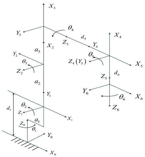
Figure 5.
The link coordinate frame of the SR4C robot.
The transformation matrix from base coordinate frame to the end-effector coordinate frame is Equations (22) and (23).
In traditional cross coupling control application, such as linear motor platforms, the transformation matrix T from tracking error to the contour error only involves the transformation of position, and the calculation is relatively simple, but traditional cross coupling control is not suitable for the robot contour control. Based on the traditional cross coupling control, an improved cross coupling controller is proposed in the local task coordinate frame. It is shown in Figure 6.
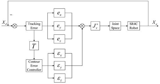
Figure 6.
Cross coupled control based on the local task coordinate frame.
The contour error control flow chart based on the control block diagram of Figure 6 is showed in Figure 7.
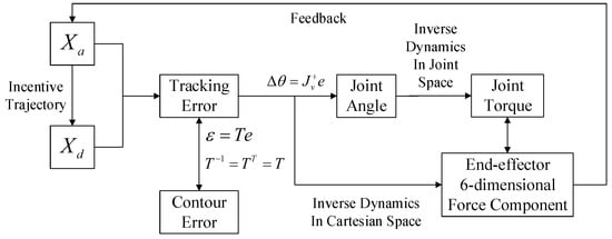
Figure 7.
Control flow chart of the contour error.
The controller proposed in the literature [23] is shown in Figure 8.
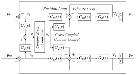
Figure 8.
Block diagram of the typical cross-coupled control system.
In Figure 7, first, we get the corresponding point on the desired trajectory according to the parameter value of the NURBS curve corresponding to point on the actual trajectory, and the tracking error from point to point could be calculated. The contour error at point D is obtained from Equation (21). Then, the end-effector coordinate frame where the tracking error locates is transformed to the joint space where each axis is located through the inverse kinematics equation of the industrial robot in Equation (22). Next, regarding the joint angle solved from Equation (22) as the input of the inverse dynamics equation in the robot joint space, and the solution of robot inverse dynamics, that is to say, joint torque as the output. At the same time, the inverse dynamics equation in joint space can be transformed to the Cartesian space, that is to say, the tracking error is taken as the input of the inverse dynamics equation. Comparing with the controller in Figure 8 which is proposed in the literature [23], controller in Figure 6, the six-dimensional force component at the end of the output is fed back to the actual trajectory, so that we could realize the closed-loop control of the contour error. Thus, the control accuracy of contour error can be improved.
The inverse dynamics equations in joint space and Cartesian space are shown in Equations (24) and (25).
where,
is the Jacobi matrix of the robot, see Equation (27),
Combining Equation (19) with (20) and (26), it can get Equation (28),
For the contour error control, . Suppose that the coordinate of the desired point is , and the coordinate of the actual point is , then the tracking error is . When D is a constant point, also becomes constant, and
Then the inverse dynamics equation in Equation (25) could be written as,
Combining Equation (10) with (11), it can get,
Substitute Equation (31) into Equation (30), we could get the dynamics equation of the robot in the local task coordinate frame, which could be expressed as,
where,
4. Analysis of Simulation Experiment Results
In this paper, SR4C robot is taken as the experimental object, and the dynamic parameters are shown in Table 2.
Table 2.
The dynamical parameter of the SR4C robot.
According to the kinetic parameters in Table 2, the kinetic equation described in Equation (24) could be calculated.
Generally speaking, a k-order NURBS curve can be expressed in the following Equation (34),
where stands for control points, ; is the weight factor corresponding to the control point, , , the rest ; is the node vector, and all the is not decrease; is the normalization factor, , ; the step size of the rest ui in the middle is , i.e., , , … ; is the k-order B-spline basis function, which is defined by the recursion Equation of Cox-de Boor as,
The parameters of the NURBS curve are as follows: the order of the NURBS curve ; the weight factor vector is ; the node vector is ; and the control points could be determined by the following Equation (36),
where, , the number of control points is ; and the step size of in Equation (36) is 0.01 rad.
Bernoulli’s lemniscate is commonly used on the robots, which is selected as the incentive trajectory, as shown in Figure 9.
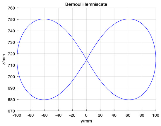
Figure 9.
Incentive trajectory.
According to Equation (36), Bernoulli’s lemniscate curve is constructed by using NURBS curve. At the same time, Bernoulli’s lemniscate curve is also constructed by using the five-order polynomial curve.
The partial enlargement of the above incentive trajectory is shown in Figure 10.
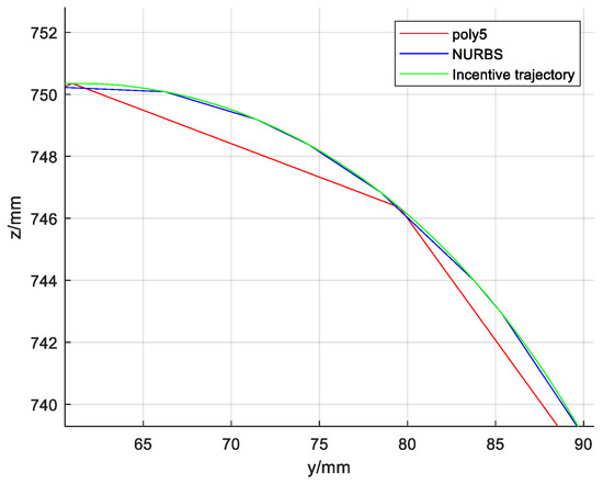
Figure 10.
Partial enlarged view of the incentive trajectory.
To evaluate the performance of the controller, the following indicators are used:
Equation (37) is the root mean square of the contour error, where is the total planning duration, which could be used for measuring the average contour error control performance.
is the maximum absolute value of the contour error, which measures the instant performance.
Figure 11 shows the uniaxial tracking error chart of the NURBS curve, Figure 12 shows the uniaxial tracking error chart of the five-order polynomial curve, and Figure 13 shows the contour error comparison chart of the NURBS curve and the five-order polynomial curve:
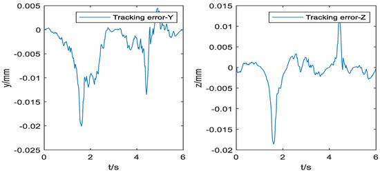
Figure 11.
Tracking error of the NURBS curve.
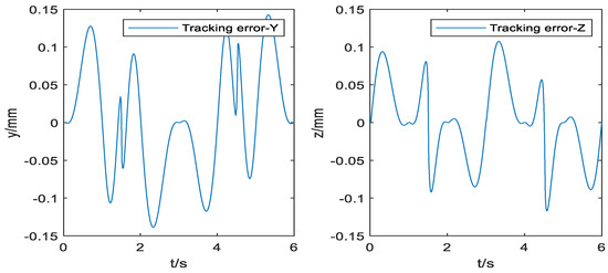
Figure 12.
Tracking error of the five-order polynomial curve.
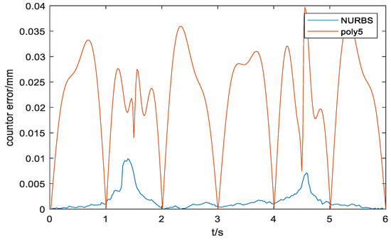
Figure 13.
Contour error comparison between the NURBS curve and the five-order polynomial curve.
The tracking error and the contour error of the NURBS curve and five-order polynomial curve can be seen in Table 3 and Table 4.
Table 3.
Error value of the NURBS curve.
Table 4.
Error value of the five-order polynomial curve.
It could be concluded from Figure 9 that the curve constructed by the NURBS curve trajectory planning is closer to the desired trajectory than the curve constructed by the five-order polynomials. Furthermore, the improved cross-coupling controller in the local task coordinate frame designed in this paper is used to control the profiles of the above two curves. Then, the single axis tracking error diagram, and the contour error result diagram of the two kinds of the two kinds of curves are obtained. Comparing Figure 10 and Figure 11, single axis tracking error curve, it is obvious that the single axis tracking error precision of the NURBS curve planning is significantly higher than the single axis tracking error precision of the five-order polynomial curve, and the single axis tracking error of the NURBS curve planning fluctuates far less than the single axis tracking error of the five-order polynomial curve.
In the comparison of the contour error curves in Figure 12, the contour error of the NURBS curve planning is significantly lower than that of the five-order polynomial curve, and the amplitude fluctuation of the NURBS curve contour error is smaller, and the fluctuation is less. Combining with the contour control data of the two curves in Table 3 and Table 4, it could be concluded that the curve constructed by the NURBS curve planning controls the contour error at the level of , and the root mean square value of the contour error decreases from of the five-order polynomial curve to of the NURBS curve.
5. Conclusions
In this paper, the difference between tracking error and contour error is described, and the significance of contour error for trajectory evaluation obtained from trajectory planning is discussed. Then, the estimation algorithm of the contour error based on the tangent approximation is proposed. Next, the estimation algorithm of the contour error in the local task coordinate frame is proposed. Then, according to the configuration characteristics of the industrial robot, an improved cross-coupling control scheme based on the local task coordinate frame is designed to control the profiles of the two incentive trajectories which are constructed by the NURBS curve and the five-order polynomial curve. The obtained uniaxial tracking error and contour error curve were compared and analyzed. Through the analysis of simulation experiment results, it is concluded that the NURBS curve has better contour control performance than the five-order polynomial curve. The research results of this manuscript provide practical application value for the high precision contouring control for industrial robots.
Author Contributions
Conceptualization, G.W. and Z.P.; methodology, G.W.; software, G.W. and J.C.; validation, G.W. and K.Z.; formal analysis, J.C.; investigation, Z.P.; resources, G.W.; data curation, K.Z.; writing—original draft preparation, G.W. and Z.P.; writing—review and editing, G.W.; visualization, J.C.; supervision, Z.P.; project administration, G.W.; funding acquisition, G.W. All authors have read and agreed to the published version of the manuscript.
Funding
This research was funded by Natural Science Foundation of Zhejiang Province, grant number LGG22F030001.
Data Availability Statement
Not applicable.
Conflicts of Interest
The authors declare no conflict of interest.
References
- Sun, J.; Han, X.; Zuo, Y.; Tian, S.; Song, J.; Li, S. Trajectory Planning in Joint Space for a Pointing Mechanism Based on a Novel Hybrid Interpolation Algorithm and NSGA-II Algorithm. IEEE Access 2020, 8, 228628–228638. [Google Scholar] [CrossRef]
- Lin, J.; Ye, C.; Yang, J.; Zhao, H.; Ding, H.; Luo, M. Contour error-based optimization of the end-effector pose of a 6 degree-of-freedom serial robot in milling operation. Robot. Comput. Manuf. 2022, 73, 102257. [Google Scholar] [CrossRef]
- Dachang, Z.; Baolin, D.; Aodong, C.; Puchen, Z. Adaptive Non-singular Terminal Sliding Mode Fault-tolerant Control of Robotic Manipulators Based on Contour Error Compensation. arXiv 2021, arXiv:2110.08705. [Google Scholar]
- Zhao, H.; Li, X.; Ge, K.; Ding, H. A contour error definition, estimation approach and control structure for six-dimensional robotic machining tasks. Robot. Comput. Manuf. 2022, 73, 102235. [Google Scholar] [CrossRef]
- Deng, K.; Gao, D.; Ma, S.; Lu, Y. Contouring Errors and Feedrate Fluctuation of Serial Industrial Robot in Complex Toolpath with Different Controller. Intell. Robot. Appl. 2021, 13013, 100–108. [Google Scholar]
- Li, K.; Boonto, S.; Nuchkrua, T. Online Self Tuning of Contouring Control for High Accuracy Robot Manipulators under Various Operations. Int. J. Control Autom. Syst. 2020, 18, 1818–1828. [Google Scholar] [CrossRef]
- Chen, R.; Li, K.; Boonto, S.; Nuchkrua, T. Contouring Control Consensus for Robot Manipulators. In Proceedings of the 2019 58th Annual Conference of the Society of Instrument and Control Engineers of Japan (SICE), Hiroshima, Japan, 10–13 September 2019. [Google Scholar]
- Kim, N.; Shim, J.; Oh, D.; Kim, H.; Lee, W. Pose optimization of robot machining system for improving position accuracy. In Proceedings of the 19th International Conference of the European Society for Precision Engineering and Nanotechnology, Bilbao, Spain, 3–7 June 2019. [Google Scholar]
- Ouyang, P.R.; Pano, V.; Acob, J. Contour Tracking Control for Multi-DOF Robotic Manipulators. In Proceedings of the 2013 10th IEEE International Conference on Control and Automation, Hangzhou, China, 12–14 June 2013. [Google Scholar]
- Li, X.; Zhao, H.; Yang, J.; Ding, H. A High Accuracy On-Line Contour Error Estimation Method of Five-axis Machine Tools. In Proceedings of the International Conference on Intelligent Robotics and Applications, ICIRA 2015, Portsmouth, UK, 24–27 August 2015; Lecture Notes in Computer Science. Springer: Cham, Swizerland, 2015. [Google Scholar]
- Su, K.-H.; Chen, H.-R.; Cheng, M.-Y. Free-form Curves Contour Error Estimation Using the Backward Arc Length Approach. In Proceedings of the 2014 IEEE/SICE International Symposium on System Integration, Tokyo, Japan, 13–15 December 2014. [Google Scholar]
- Cheng, M.-Y.; Lee, C.-C. Motion Controller Design for Contour-Following Tasks Based on Real-Time Contour Error Estimation. IEEE Ind. Electron. Mag. 2007, 54, 1686–1695. [Google Scholar] [CrossRef]
- Yeh, S.-S.; Hsu, P.-L. Estimation of the contouring error vector for the cross-coupled control design. IEEE/ASME Trans. Mechatron. 2002, 7, 44–51. [Google Scholar] [CrossRef]
- Yang, J.; Li, Z. A Novel Contour Error Estimation for Position Loop-Based Cross-Coupled Control. IEEE/ASME Trans. Mechatron. 2011, 16, 643–655. [Google Scholar] [CrossRef]
- Hu, C.; Hu, Z.; Zhu, Y.; Wang, Z. Advanced GTCF-LARC Contouring Motion Controller Design for an Industrial X–Y Linear Motor Stage With Experimental Investigation. IEEE Trans. Ind. Electron. 2017, 64, 3308–3318. [Google Scholar] [CrossRef]
- Zheng, M.; Zhang, F.; Zhu, J.; Zuo, Z. A fast and accurate bundle adjustment method for very large-scale data. Comput. Geosci. 2020, 142, 104539. [Google Scholar] [CrossRef]
- Huo, F.; Poo, A.N. Free-form Two-dimensional Contour Error Estimation Based on NURBS Interpolation. In Proceedings of the Applied Mechanics and Materials. Trans. Tech. Publ. 2012, 157, 236–240. [Google Scholar]
- Biagiotti, L.; Califano, F.; Melchiorri, C. Repetitive Control Meets Continuous Zero Phase Error Tracking Controller for Precise Tracking of B-Spline Trajectories. IEEE Trans. Ind. Electron. 2020, 67, 7808–7818. [Google Scholar] [CrossRef]
- Jin, Z.; Cheng, G.; Meng, Y. Feedforward Combined Multi-axis Cross-coupling Contour Control Compensation Strategy of Optical Mirror Processing Robot. Robotica 2022, 40, 3476–3498. [Google Scholar] [CrossRef]
- Wang, L.; Kong, X.; Yu, G.; Li, W.; Li, M.; Jiang, A. Error Estimation and Cross-coupled Control Based on a Novel Tool PoseRepresentation Method of a Five-axis Hybrid Machine Tool. Int. J. Mach. Tools Manuf. 2022, 182, 103955. [Google Scholar] [CrossRef]
- Wang, S.; Chen, Y.; Zhang, G. Adaptive fuzzy PID cross coupled control for multi-axis motion system based on sliding mode disturbance observation. Sci. Prog. 2021, 104, 1–19. [Google Scholar] [CrossRef]
- Hu, N.T.; Chen, L.Y.; Chen, C.S. Novel Cross-coupling Position Command Shaping Controller using in Multi-axis Motion Systems. IEEE Trans. Ind. Electron. 2022, 69, 13099–13110. [Google Scholar] [CrossRef]
- Li, B.; Wang, T.; Wang, P. Cross-coupled Control Based on Real-time Double Circle Contour Error Estimation for Biaxial Motion System. Meas. Control 2021, 54, 324–335. [Google Scholar]
- Ji, W.; Cui, X.; Xu, B.; Ding, S.; Ding, Y.; Peng, J. Cross-coupled Control for Contour Tracking Error of Free-form Curve Based on Fuzzy PID Optimized by Im-proved PSO Algorithm. Meas. Control 2022, 55, 807–820. [Google Scholar] [CrossRef]
- Jiang, Y.; Chen, J.; Zhou, H.; Yang, J.; Hu, P.; Wang, J. Contour error modeling and compensation of CNC machining based on deep learning and reinforcement learning. Int. J. Adv. Manuf. Technol. 2022, 118, 551–570. [Google Scholar] [CrossRef]
- Wang, Z.; Hu, C.; Zhu, Y. Accelerated Iteration Algorithm Based Contouring Error Estimation for Multiaxis Motion Control. IEEE/ASME Trans. Mechatron. 2022, 27, 452–462. [Google Scholar] [CrossRef]
- Wu, J.; Xiong, Z.; Ding, H. Integral design of contour error model and control for biaxial system. Int. J. Mach. Tools Manuf. 2015, 89, 159–169. [Google Scholar] [CrossRef]
- Alandoli, E.A.; Lee, T.; Vijayakumar, V.; Lin, Y.; Mohammed, M.Q. Dynamic model and integrated optimal controller of hybrid arms robot for laser contour machining. J. Vib. Control 2022, 1–19. [Google Scholar] [CrossRef]
- Zhang, X.; Lu, W.; Su, M.; Xu, W. Research on Synchronous Control Strategy of Robot Arm Based on Cross-Coupling Control. Int. J. Innov. Comput. Inf. Control 2020, 16, 1987–2005. [Google Scholar]
- Nuchkrua, T.; Kornmaneesang, W.; Chen, S.L.; Boonto, S. Precision Contouring Control of 5 DOF Dual-arm Robot Manipulators with Holonomic Constraints. In Proceedings of the 2017 11th Asian Control Conference (ASCC), Gold Coast, Australia, 17–20 December 2017. [Google Scholar]
- Xu, G.; Zhang, H.; Meng, Z.; Sun, Y. Automatic interpolation algorithm for NURBS trajectory of shoe sole spraying based on 7-DOF robot. Int. J. Cloth. Sci. Technol. 2022, 34, 434–450. [Google Scholar] [CrossRef]
- Zhang, H.; Ni, X.; Hu, P.; Yuan, Y. Real-Time Contour Error Estimation with NURBS Interpolator. In Proceedings of the 2018 2nd International Conference on Robotics and Automation Sciences (ICRAS), Beijing, China, 23–25 June 2018. [Google Scholar]
- Erwinski, K.; Paprocki, M.; Wawrzak, A.; Grzesiak, L.M. Pso Based Feedrate Optimization with Contour Error Constraints for NURBS Toolpaths. In Proceedings of the 2016 21st International Conference on Methods and Models in Automation and Robotics (MMAR), Miedzyzdroje, Poland, 29 August–1 September 2016. [Google Scholar]
- Wu, G.; Zhao, W.; Zhang, X. Optimum time-energy-jerk trajectory planning for serial robotic manipulators by reparameterized quintic NURBS curves. Proc. Inst. Mech. Eng. Part C J. Mech. Eng. Sci. 2021, 235, 4382–4393. [Google Scholar] [CrossRef]
- Erwinski, K.; Wawrzak, A.; Paprocki, M. Real-Time Jerk Limited Feedrate Profiling and Interpolation for Linear Motor Multiaxis Machines Using NURBS Toolpaths. IEEE Trans. Ind. Inform. 2022, 18, 7560–7571. [Google Scholar] [CrossRef]


Publisher’s Note: MDPI stays neutral with regard to jurisdictional claims in published maps and institutional affiliations. |
© 2022 by the authors. Licensee MDPI, Basel, Switzerland. This article is an open access article distributed under the terms and conditions of the Creative Commons Attribution (CC BY) license (https://creativecommons.org/licenses/by/4.0/).