Analysis of the Type V Intermittency Using the Perron-Frobenius Operator

Abstract

A methodology to study the reinjection process in type V intermittency is introduced. The reinjection probability density function (RPD), and the probability density of the laminar lengths (RPDL) for type V intermittency are calculated. A family of maps with discontinuous and continuous RPD functions is analyzed. Several tests were performed, in which the proposed technique was compared with the classical theory of intermittency, the M function methodology, and numerical data. The analysis exposed that the new technique can accurately capture the numerical data. Therefore, the scheme presented herein is a useful tool to theoretically evaluate the statistical variables for type V intermittency.

1. Introduction

Dynamical systems model numerous phenomena, processes, and mechanisms, that can evolve into chaos using different routes. One of these routes is chaotic intermittency, where a dynamical system solution alternates chaotic bursts with laminar or regular phases. The regular phases correspond with pseudo-equilibrium regions or pseudo-periodic solutions, but at the bursts the evolution is chaotic [1,2,3,4].

Classic chaotic intermittency was grouped into three types, I, II and III, according to the periodic orbit stability loss evaluated by the Floquet multipliers, or to the fixed point loss of stability evaluated by the eigenvalues of the map. Subsequent papers introduced other types of intermittencies: on–off (in–out), V, X, eyelet, and ring [5,6,7,8,9,10].

We emphasize that a more complete understanding of chaotic intermittency could expand its application to various fields of study, due to previous experiences observed in physics, chemistry, medicine, and economics [11,12,13,14,15,16,17,18,19,20,21].

One-dimensional maps are widely utilized to analyze chaotic intermittency [1,2,3,4,22]. Maps with intermittency are characterized by a local map that determines the intermittency type, and a non-linear map that generates the reinjection process. The reinjection probability density function (RPD) is utilized to describe the reinjection process, and establishes the probability of the trajectories to be reinjected in the laminar interval [1,4]. Accordingly, the proper calculation of the RPD function is fundamental to accurately outline the chaotic intermittency phenomenon. There was no universal methodology to determine the RPD, and distinct methods were used of which the uniform reinjection mechanism (constant RPD function) was the most utilized [1,2,3,22]. However, a more extensive methodology to calculate the RPD function, the M function, has been developed over the last decade. It has accurately worked for different maps with types I, II, III, and V intermittencies [23,24,25,26,27].

Type V intermittency was previously described in the literature by [28,29,30], and occurs when a fixed point loses its stability via a collision with a non-differentiable point (NDP) forming a channel between the bisector line and the map. However, at this point, the local map is non-differentiable or discontinuous and there is no tangent bifurcation. More recent studies to calculate the RPD in type V intermittency are presented in Refs. [26,27]. Applications of type V intermittency can be found in neuronal activity studies [31,32,33]. For example, in the Hindmarsh–Rose model, there is an intermittent behavior between irregular bursting and laminar phases close to a period-3 bursting [32].

In this paper, we utilize the Perron–Frobenius operator to elaborate a methodology to compute the reinjection probability density function and the probability density of the laminar lengths (RPDL) for type V intermittency [34,35]. Hereafter, this methodology is referred to as the continuity technique. To validate the continuity technique in order to evaluate the RPD and RPDL functions for type V intermittency, a family of maps is analyzed. Comparisons between analytical results calculated using this technique, the classical theory of intermittency, the M function methodology, and numerical data are carried out. Finally, the advantages and drawbacks of the continuity technique are described.

2. Study of Type V Intermittency

Prior to discussing the application to type V intermittency, a short description about the evolution of densities is necessary (the Perron–Frobenius operator). A more complete and deeper explanation of this subject can be found in Refs. [36,37]. We consider a family of evolution operators $F^t\left(x\right):D\to D$, such as $F^{t_1+t_2}=F^{t_1}\circ F^{t_2}$ and $F^0=$ identity, $x\in D$, being D a compact manifold, and t the evolution variable. If t varies over the real numbers ($t\in \mathbb{R}$), $F^t\left(x\right)$ represents a dynamical system. Nevertheless, if t acquires exclusively discrete values, the operator $F^t\left(x\right)$ is a map. There are, at least, two formulations to explain the functioning of $F^t\left(x\right)$. One alternative is to analyze the trajectories evolution, the other considers the density and the probability measure concepts.

Let us introduce a map $y=F\left(x\right)$, that transforms some interval $\mathrm{\Delta }\subset \mathbb{R}$ into another interval ${\mathrm{\Delta }}_a\subset \mathbb{R}$. Hence, $x\in \mathrm{\Delta }$ and $y\in {\mathrm{\Delta }}_a$. In $\mathrm{\Delta }$, the density of trajectories can be defined as $\rho \left(x\right)$, while in ${\mathrm{\Delta }}_a$ the trajectories density is ${\rho }_a\left(y\right)$. We can transform the density $\rho$ in ${\rho }_a$, and we write ${\rho }_a=\mathcal{L}\circ \rho$. If we consider $\mathrm{\Delta }=[y_0,y]$, where the upper limit y is variable, the density ${\rho }_a\left(y\right)$ results

$${\rho }_a\left(y\right)=\frac{d}{dy}{\int }_{F^{-1}[y_0,y]}\rho \left(x\right)\mathrm{d}x=\rho \left(F^{-1}\left(y\right)\right)\left|\frac{d{F}^{-1}\left(y\right)}{dy}\right|.$$

(1)

This equation assumes that $F\left(x\right)$ is piecewise differentiable and invertible. Furthermore, the derivative $\frac{d{F}^{-1}\left(x\right)}{dx}$ is piecewise continuous [36].

To apply Equation (1) in type V intermittency, we introduce the following family of maps

$$F\left(x\right)=\left\{\begin{array}{cc}{F}_1\left(x\right)={\lambda }_{1}x+\epsilon \hfill & \widehat{x}\le x<0,\hfill \\ F_2\left(x\right)=\epsilon +x+{\lambda }_2{x}^2\hfill & 0\le x<x_m,\hfill \\ F_3\left(x\right)=\widehat{x}+\frac{(y_m-\widehat{x}){(y_m-x)}^{\gamma }}{{(y_m-x_m)}^{\gamma }}\hfill & x_m\le x\le y_m,\hfill \end{array}\right.$$

(2)

where $y_m=F\left(x_m\right)=1$, $\epsilon$ is the control parameter, ${\lambda }_1$ is the slope of the straight line ($0<{\lambda }_1<1$), ${\lambda }_2$ is the quadratic term coefficient in $F_2\left(x\right)$, $\gamma$ is the exponent in $F_3\left(x\right)$, and $\widehat{x}$ is the lower boundary of reinjection [4]. For $\epsilon =0$, $x_0=0$ is a fixed point of the map, and for $0<\epsilon \ll 1$ type V intermittency occurs. To carry out a more general study, this family of maps does not have symmetry around the fixed point, and it can generate type V intermittency with continuous and discontinuous RPD functions.

If we apply Equation (1) to the map given by Equation (2), for the sub-interval $[\widehat{x},F_1\left(\widehat{x}\right))$ we obtain

$$\mathcal{L}\circ \rho \left(x\right)=\rho \left(F_3^{-1}\left(x\right)\right)\left|\frac{d{F}_3^{-1}\left(x\right)}{dx}\right|,$$

(3)

for the sub-interval $[F_1\left(\widehat{x}\right),0)$ results

$$\mathcal{L}\circ \rho \left(x\right)=\rho \left(F_1^{-1}\left(x\right)\right)\left|\frac{d{F}_1^{-1}\left(x\right)}{dx}\right|+\rho \left(F_3^{-1}\left(x\right)\right)\left|\frac{d{F}_3^{-1}\left(x\right)}{dx}\right|,$$

(4)

and for the sub-interval $[0,y_m]$ we have

$$\mathcal{L}\circ \rho \left(x\right)=\rho \left(F_2^{-1}\left(x\right)\right)\left|\frac{d{F}_2^{-1}\left(x\right)}{dx}\right|+\rho \left(F_3^{-1}\left(x\right)\right)\left|\frac{d{F}_3^{-1}\left(x\right)}{dx}\right|.$$

(5)

Figure 1 shows how the intervals are mapped to obtain Equations (3)–(5). Blue, red, and green arrows correspond to Equations (3)–(5), respectively. Furthermore, Figure 1 and Equations (4) and (5) show that there is symmetry in the process of density evolution.

On the other hand, for a map $F\left(x_n\right):H\to H$ where $H\subset \mathbb{R}$, the probability measure of an interval $S\subset H$ can be written as

$$P\left(S\right)=\underset{N\to \infty }{lim}\frac{1}{N}\sum _{n=0}^N{I}_S\left(x_n\right),$$

(6)

where $I_S\left(x\right)$ is the characteristic function of the interval S

$$I_S\left(x\right)=\left\{\begin{array}{ccc}1,\hfill & \mathrm{if}& x\in S\\ 0,\hfill & \mathrm{if}& x\notin S.\end{array}\right.$$

(7)

Consequently, the probability measure indicates the frequency that the trajectory reaches the corresponding interval, and is related to the invariant density $\rho \left(x\right)$ by

$$P\left(S\right)={\int }_S\rho \left(x\right)dx.$$

(8)

Let $L\equiv S$ be the laminar region. Before considering the probability $P\left(L\right)$ given by Equation (6), we divide the whole data series into three subsets

$$\left\{x_n\right\}=\left\{x_{n^{\prime }}\right\}\cup \left\{x_{n^{″}}\right\}\cup \left\{x_{n^{‴}}\right\}.$$

(9)

First, we choose $x_{n^{\prime }}\in L$, and in the preceding iteration it has already been there, that is $I_L\left(x_{n^{\prime }}\right)=1$ and $I_L\left(x_{n^{\prime }-1}\right)=1$. Furthermore, we have $x_{n^{″}}\in L$ but in the preceding iteration it has not been there, that is $I_L\left(x_{n^{″}}\right)=1$ and $I_L\left(x_{n^{″}-1}\right)=0$. Finally, $x_{n^{‴}}\notin L$. It is notable that there exists no intersection between them

$$\left\{x_{n^{\prime }}\right\}\cap \left\{x_{n^{″}}\right\}=\left\{x_{n^{″}}\right\}\cap \left\{x_{n^{‴}}\right\}=\left\{x_{n^{‴}}\right\}\cap \left\{x_{n^{\prime }}\right\}=Ø.$$

(10)

Therefore, $P\left(L\right)$ is

$$P\left(L\right)=\underset{N\to \infty }{lim}\frac{1}{N}\sum _{n^{\prime }=0}^N{I}_L\left(x_{n^{\prime }}\right)+\underset{N\to \infty }{lim}\frac{1}{N}\sum _{n^{″}=0}^N{I}_L\left(x_{n^{″}}\right),$$

(11)

The first term in Equation (11) is the probability for the trajectory to be in L when in the preceding iteration it has already been there. Subsequently, only the second term in the RHS of Equation (11) defines the RPD function, denoted here by $\varphi \left(x\right)$, by means of the following relation

$$\underset{N\to \infty }{lim}\frac{1}{N}\sum _{n^{″}=0}^N{I}_L\left(x_{n^{″}}\right)=w{\int }_L\varphi \left(x\right)\mathrm{d}x,$$

(12)

where the weight w is introduced because it is common to normalize the function $\varphi \left(x\right)$ over the whole laminar interval L as ${\int }_L\varphi \left(x\right)dx=1$. Next, to evaluate the RPD function the sums in Equation (3)–(5) have to exclude the contributions that do not produce reinjection inside of the laminar interval [4,35]

$$\varphi \left(x\right)=\sum _{j\ne l}^n\left|\frac{d{F}_j^{-1}\left(x\right)}{dx}\right|\rho \left(F_j^{-1}\left(x\right)\right),$$

(13)

where l indicates the integrals that do not generate reinjection and $\rho \left(F_j^{-1}\left(x\right)\right)$ is the density in the preceding iteration to reinjection. The normalization condition is

$$\sum _{j\ne l}^n{\int }_{{F_j}^{-1}(x_0-c)}^{{F_j}^{-1}(x_0+c)}\rho \left(F_j^{-1}\left(x\right)\right)\mathrm{d}x=1,$$

(14)

where c is the semi-amplitude of the laminar interval, and $x_0$ is the fixed point, $L=[x_0-c,x_0+c]$.

2.1. Continuous RPD

Let us consider the lower boundary of reinjection in the family of maps described by Equation (2) with $\widehat{x}=x_0-c$, $x_0=0$, and $y_m=1$. Therefore, there is no reinjection from points $x<x_0-c$ because the lower limit of the laminar interval is the lower boundary of reinjection. To obtain the RPD function we use Equations (13) and (14). Note that $F_1\left(x\right)$ and $F_2\left(x\right)$ do not produce reinjection, and the RPD can then be calculated as

$$\varphi \left(x\right)=\rho \left(F_3^{-1}\left(x\right)\right)\left|\frac{d{F}_3^{-1}\left(x\right)}{dx}\right|,$$

(15)

where

$$\left|\frac{d{F}_3^{-1}\left(x\right)}{dx}\right|=\frac{(1-x_m){(x+c)}^{1/\gamma -1}}{\gamma {(1+c)}^{1/\gamma }}.$$

(16)

To apply Equation (15) we have to evaluate the density at pre-reinjection points, $\rho \left(F_3^{-1}\left(x\right)\right)$. Let us expand $\rho$ by a Taylor series around the pre-image of the lower boundary of the reinjection $F_3^{-1}(-c)$. Using the notation $y=F_3^{-1}\left(x\right)$ and $y_{-c}=F_3^{-1}(-c)$ we get

$$\rho \left(y\right)=\rho \left(y_{-c}\right)+{\left.\frac{d\rho \left(y\right)}{dy}\right|}_{y=y_{-c}}(y-y_{-c})+\frac{1}{2}{\left.\frac{d^2\rho \left(y\right)}{d{y}^2}\right|}_{y=y_{-c}}{(y-y_{-c})}^2+\dots .$$

(17)

Using the normalization condition, Equation (14), we obtain

$$\begin{array}{cc}\rho \left(y\right)\cong \hfill & \frac{1}{\mathrm{\Delta }y\left(c\right)}+{\left.\frac{d\rho \left(y\right)}{dy}\right|}_{y=y_{-c}}\left(\mathrm{\Delta }y\left(x\right)-\frac{\mathrm{\Delta }y\left(c\right)}{2}\right)\hfill \\ \hfill & +{\left.\frac{d^2\rho \left(y\right)}{d{y}^2}\right|}_{y=y_{-c}}\left(\frac{\mathrm{\Delta }{y}^2\left(x\right)-\frac{\mathrm{\Delta }{y}^2\left(c\right)}{3}}{2}\right),\hfill \end{array}$$

(18)

where we define $\mathrm{\Delta }y\left(x\right)=F_3^{-1}(-c)-F_3^{-1}\left(x\right)$, hence we have $\mathrm{\Delta }y\left(c\right)=F_3^{-1}(-c)-F_3^{-1}\left(c\right)$.

As $c<<1$, the family of maps described by Equation (2) verifies that $\mathrm{\Delta }y\left(x\right)<\mathrm{\Delta }y\left(c\right)<<1$. Note that for $c=0.05$, the linear term has the same magnitude as the first one in the Taylor series if the derivative ${\left.\frac{d\rho \left(y\right)}{dy}\right|}_{y=y_{-c}}$ is approximately one order of magnitude greater than the first term, $\frac{1}{\mathrm{\Delta }y\left(c\right)}$. Following a similar analysis, the second derivative, ${\left.\frac{d^2\rho \left(y\right)}{d{y}^2}\right|}_{y=y_{-c}}$ has to be approximately two orders of magnitude greater than the first term in the series. Furthermore, from Equations (15) and (18) the RPD can be written as

$$\begin{array}{cc}\varphi \left(x\right)\cong \hfill & \left(\frac{1}{\mathrm{\Delta }y\left(c\right)}+{\left.\frac{d\rho \left(y\right)}{dy}\right|}_{y=y_{-c}}\left(\mathrm{\Delta }y\left(x\right)-\frac{\mathrm{\Delta }y\left(c\right)}{2}\right)\right)\left|\frac{dy}{dx}\right|\hfill \\ \hfill & +\left({\left.\frac{d^2\rho \left(y\right)}{d{y}^2}\right|}_{y=y_{-c}}\left(\frac{\mathrm{\Delta }{y}^2\left(x\right)-\frac{\mathrm{\Delta }{y}^2\left(c\right)}{3}}{2}\right)\right)\left|\frac{dy}{dx}\right|.\hfill \end{array}$$

(19)

If the derivative $\left|\frac{dy}{dx}\right|=\left|\frac{d{F}_3^{-1}\left(x\right)}{dx}\right|$ has very high or close to zero values, and the variation generated by the linear and quadratic terms in Equation (18) is not really significant in comparison with the first term, $\frac{1}{\mathrm{\Delta }y\left(c\right)}$, they do not significantly modify the RPD. Therefore, the first term in Equation (18) can be considered the most important, and we can assume that

$$\rho \left(F_3^{-1}\left(x\right)\right)\cong \frac{1}{F_3^{-1}(-c)-F_3^{-1}\left(c\right)}=\frac{1}{1-x_m}{\left(\frac{1+c}{2c}\right)}^{1/\gamma },$$

(20)

then the RPD results

$$\varphi \left(x\right)=\frac{{(x+c)}^{1/\gamma -1}}{\gamma {\left(2c\right)}^{1/\gamma }}.$$

(21)

This is a power function with exponent $\alpha =\frac{1}{\gamma }-1$. This same result was calculated using the M function methodology [27].

To validate the new theoretical evaluations, we perform a comparison between the RPDs here obtained with numerical data, with those calculated by the M function methodology and with the classical theory of intermittency. A detailed explanation of the M function methodology can be found in Refs. [4,23,24,25], and is not described here. On the other hand, the classical theory uses a constant RPD to describe the reinjection process, i.e., uniform reinjection (see Refs. [1,3,4,22]). To obtain the numerical data, we produce an iterative process for the map and also split the laminar interval into $N_s$ sub-intervals. After that, we calculate the histogram of reinjections and the numerical RPD. To obtain the histogram we consider at least $10N_s$ reinjections, which indicates millions of iterations.

For all tests in this section, the following parameters are used $a_1=0.9$, $a_2=1$, and $\widehat{x}=-c$. Thus, the reinjection process is driven only by $F_3\left(x\right)$. The reinjected points in the laminar interval, $L=[x_0-c,x_0+c]$, are mapped only by $F_3\left(x\right)$ from points in the interval $I_3\left(x\right)=[F_3^{-1}(x_0-c),F_3^{-1}(x_0+c)]$. For the first test, we also use $\gamma =1$, $\epsilon =0.001$, and $c=0.05$. To obtain the RPD function, we consider Equation (21), and it results

$$\varphi \left(x\right)=\frac{1}{2c}.$$

(22)

To validate this result, we conduct a complete set of numerical simulations for a different number of reinjected points N, and we divide the laminar interval into $N_s$ sub-intervals, where the RPDs are evaluated. To analyze the difference between numerical data and the theoretical RPD given by Equation (22), we calculate

$$D_r=\sqrt{\frac{{\sum }_{j=1}^{j=N_s}\frac{{({\varphi }_t\left(j\right)-{\varphi }_n\left(j\right))}^2}{{\left({\varphi }_t\left(j\right)\right)}^2}}{N_s^2}},E_r=\frac{{\sum }_{j=1}^{j=N_s}\frac{|{\varphi }_t\left(j\right)-{\varphi }_n\left(j\right)|}{{\varphi }_t\left(j\right)}}{N_s},$$

(23)

where ${\varphi }_n\left(j\right)$ and ${\varphi }_t\left(j\right)$ are the numerical and theoretical values of the RPD in the sub-interval j. Note that $D_r,E_r\ge 0$.

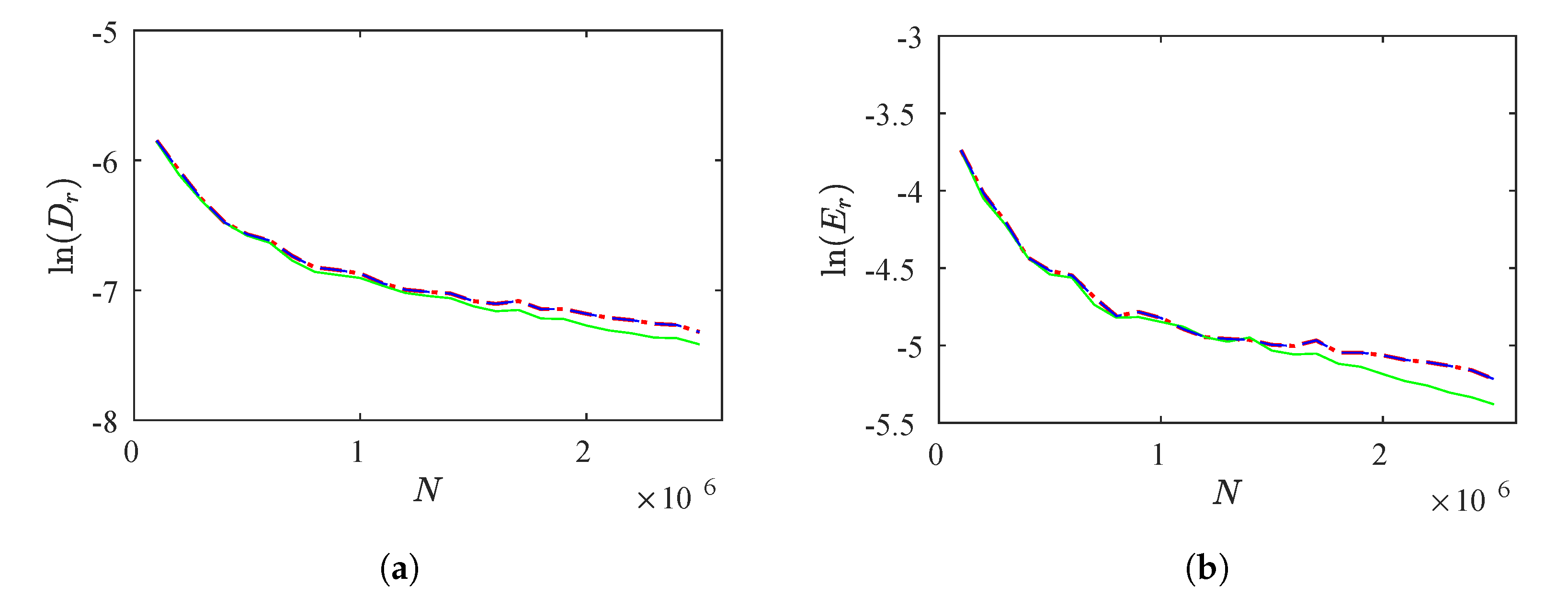
Figure 2a,b show $ln\left(D_r\right)$ and $ln\left(E_r\right)$ for a different number of reinjected points, N from $5\times {10}^4$ to $25\times {10}^5$ with $N_s=100$. We highlight that as the number of reinjected points grows, the differences between the theoretical formulations and the numerical data decrease. Notice that the M function methodology calculates $\alpha \approx 0$. 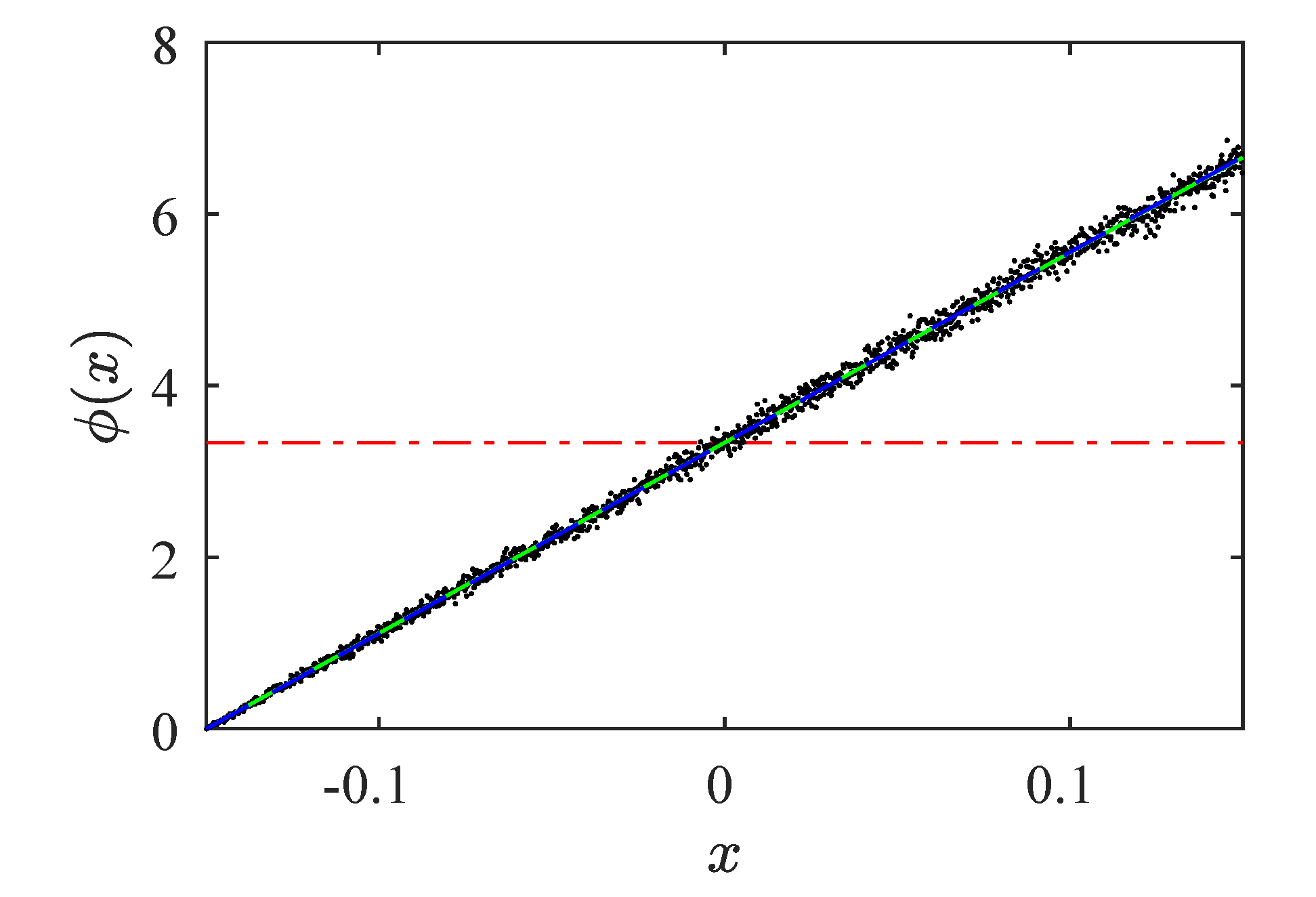This result coincides with Equation (22). Numerical and theoretical RPDs are shown in Figure 3. From Figure 2a,b and Figure 3 we observe a good agreement between the RPD functions.

To evaluate the rate of convergence, we utilize the sequence ${\left\{\frac{1}{N^p}\right\}}_{N=1}^{\infty }$ that converges to zero for $p>0$ (N are positive integer numbers), and we must verify

$$D_r\le K_d\frac{1}{N^{p_d}},E_r\le K_e\frac{1}{N^{p_e}},$$

(24)

for $K_d$, $K_e$, $p_d$ and $p_e$ fixed positive real numbers. Therefore, ${\left\{D_r\right\}}_{N=1}^{\infty }$ and ${\left\{E_r\right\}}_{N=1}^{\infty }$ converge to zero with order, or rate, of convergence $O\left(\frac{1}{N^{p_d}}\right)$ and $O\left(\frac{1}{N^{p_e}}\right)$, respectively, [38]. For this test we obtain $p_d\approx p_e\approx 0.45$. Subsequently, $D_r$ and $E_r$ converge to zero for $N\to \infty$.

The parameters $\gamma =0.5$, $\epsilon =0.005$, and $c=0.15$ are utilized for the second test. By Equation (21) we obtain

$$\varphi \left(x\right)=\frac{(x+c)}{2c^2}=50(x+0.1).$$

(25)

The calculated RPD using the M function methodology is [27]

$$\varphi \left(x\right)=48.99{(x+0.1)}^{0.9999}.$$

(26)

Figure 4a,b show $ln\left(D_r\right)$ and $ln\left(E_r\right)$ for a number of reinjected points, respectively. For these figures, we use N from $5\times {10}^4$ to $25\times {10}^5$ and $N_s=1500$. We can observe that the differences between RPDs calculated with the continuity technique and the M function methodology with numerical data decrease while N increases. However, this behavior is not verified by the classical RPD.

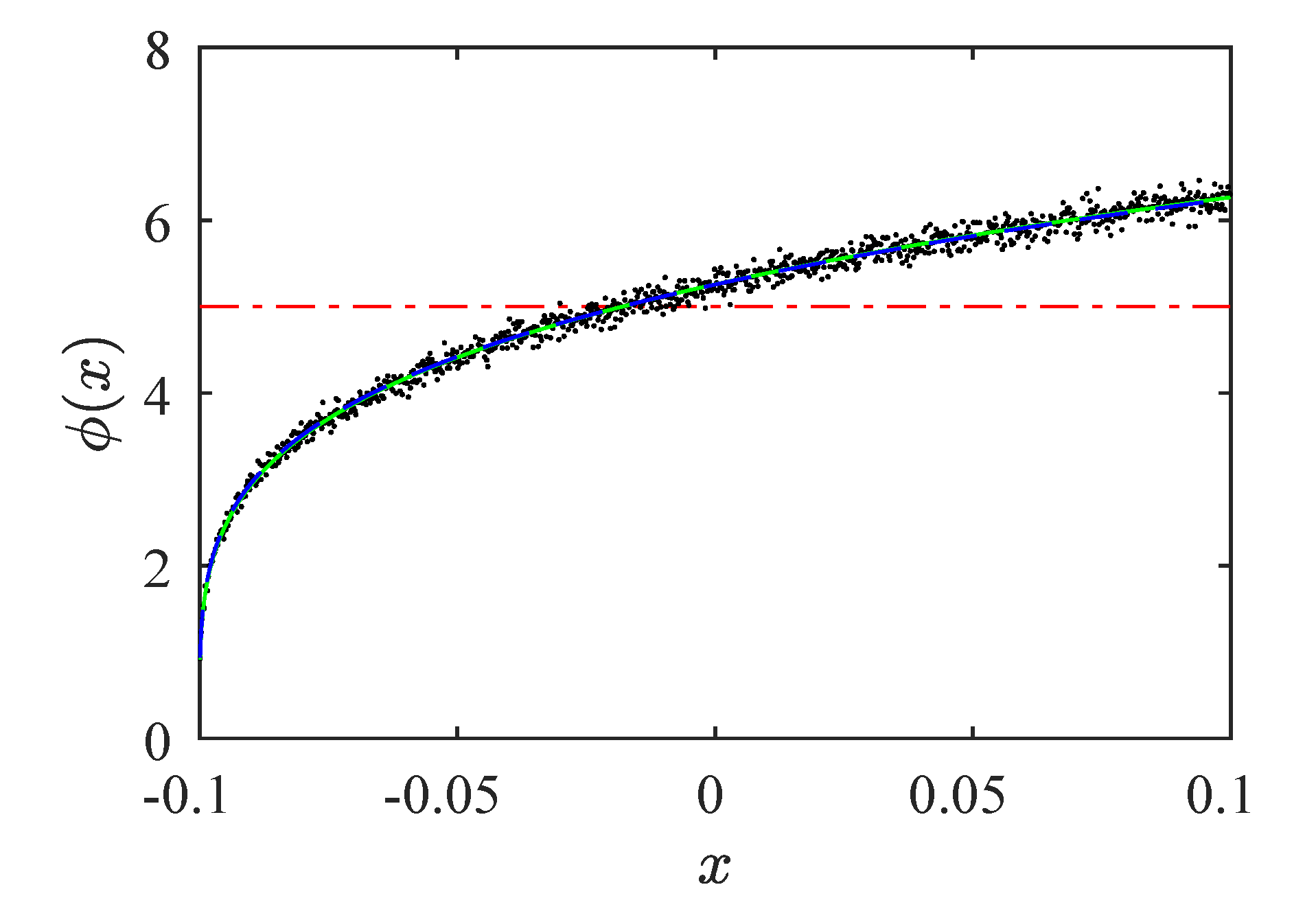
Figure 5 shows the comparison between theoretical and numerical RPDs. From this figure, and Figure 4a,b we note that the classical theory does not obtain correct results for this test. However, we observe that both methodologies, M function, and continuity, work better than classical theory, capture the numerical data, and $D_r$ and $E_r$ decrease while N increases. For the continuity technique, we find that $p_d\approx p_e\approx 0.45$; therefore, $D_r$ and $E_r$ converge to zero for $N\to \infty$.

For the third test, we use $\gamma =0.8$, $\epsilon =0.01$, $c=0.1$, N from $5\times {10}^4$ to $30\times {10}^5$ and $N_s=1000$. From Equation (21) we calculate

$$\varphi \left(x\right)=9.346{(x+0.1)}^{0.25}.$$

(27)

The M function methodology obtains

$$\varphi \left(x\right)=9.414{(x+0.1)}^{0.253}.$$

(28)

Figure 6a,b show $ln\left(D_r\right)$ and $ln\left(E_r\right)$ vs. the number of reinjected points for N from $5\times {10}^4$ to $3\times {10}^6$. We observe that the $D_r$ and $E_r$ calculated with continuity and M function methodologies decrease while N increases. Again, this behavior is not obtained for the classical RPD.

The RPD functions are shown in Figure 7. We note that the RPDs calculated with the continuity and M function methodologies adequately represent the numerical data. However, the classical RPD function cannot accurately reproduce the numerical data. If we use Equation (24) for the continuity technique, we obtain $p_d\approx 0.5$ and $p_e\approx 0.45$, i.e., $D_r$ and $E_r$ converge to zero for $N\to \infty$.

The fourth test uses $\gamma =1.5$, $\epsilon =0.0001$, $c=0.015$, N from $5\times {10}^4$ to $25\times {10}^5$ and $N_s=1000$. From Equation (21) we calculate

$$\varphi \left(x\right)=6.905{(x+0.015)}^{-1/3}.$$

(29)

The M function methodology obtains

$$\varphi \left(x\right)=7.091{(x+0.015)}^{-0.328}.$$

(30)

The $ln\left(D_r\right)$ and $ln\left(E_r\right)$ are shown in Figure 8a,b for N from $5\times {10}^4$ to $25\times {10}^5$ and $N_s=1000$. We observe that the $D_r$ and $E_r$ calculated with continuity and M function methodologies decrease for increasing N. Similar to the previous tests, the classical theory obtains poor results. For the RPD function calculated by the continuity methodology, we obtain $p_d\approx 0.4$ and $p_e\approx 0.45$, then $D_r$ and $E_r$ converge to zero for $N\to \infty$ (see Equation (24)).

Figure 9 shows the RPDs functions. The RPDs calculated using the continuity and M function methodologies can describe the numerical data behavior. On the other hand, the classical RPD function cannot accurately reproduce the numerical data.

For the fifth test, we consider $\gamma =2$, $\epsilon =0.0005$, $c=0.02$, and $N_s=2000$. If we use the continuity technique, Equation (21), we obtain

$$\varphi \left(x\right)=2.5{(x+0.02)}^{-0.5}.$$

(31)

The RPD calculated using the M function methodology is

$$\varphi \left(x\right)=2.474{(x+0.02)}^{-0.502}.$$

(32)

For $N=5\times {10}^4-25\times {10}^5$, Figure 10a,b show $ln\left(D_r\right)$ and $ln\left(E_r\right)$. From these figures, we observe that for the continuity technique and the M function methodology $D_r$ and $E_r$ decrease whereas N increases. However, $D_r$ and $E_r$ are approximately constant for the classical theory. For the RPD given by Equation (31), we obtain that $p_d\approx 0.35$ and $p_e\approx 0.4$, accordingly $D_r,E_r\to 0$ for $N\to \infty$.

The RPD functions are shown in Figure 11. The RPDs calculated by the M function methodology and continuity technique reproduce the numerical results whereas classical theory does not.

The results for the five sets of tests are summarized in

Table 1. Results for the five sets of tests with continuous RPD functions.

$\mathit{\epsilon }$	$\mathit{\gamma }$	c	${\mathit{N}}_{\mathit{s}}$	${\mathit{p}}_{\mathit{e}}$	${\mathit{p}}_{\mathit{d}}$
$0.001$	$1.0$	$0.05$	100	$0.45$	$0.45$
$0.005$	$0.5$	$0.15$	1500	$0.45$	$0.45$
$0.010$	$0.8$	$0.10$	1000	$0.45$	$0.50$
$0.0001$	$1.5$	$0.015$	1000	$0.45$	$0.40$
$0.0005$	$2.0$	$0.02$	2000	$0.40$	$0.35$

. In these tests, we use different values of the exponent $\gamma$, the length of the laminar interval c, the parameter $\epsilon$, and the number of sub-intervals $N_s$, despite that in all these tests for the continuity technique $D_r$ and $E_r$ diminish as the number of re-injected points increases, showing that the theoretical evaluation given by Equation (21) approximates with more accuracy the numerical RPD as the number of reinjected points increases. For all tests, the convergence process verifies $0.35<p_d<0.5$ and $0.4<p_e<0.45$. Furthermore, from the tests we highlight that the continuity technique works better than the classical theory, and obtains RPD functions with approximately the same accuracy as the M function methodology. In addition, the continuity technique has the advantage of being able to predict analytic RPD functions knowing only the map without using numerical or experimental data.

Only the first and second tests produce symmetric RPD functions around the fixed point. For $\gamma \ne 0.5$ and $\gamma \ne 1$ the symmetry is lost.

Note that to obtain the previous results, we have assumed a constant density at pre-reinjection points. This assumption is based on two concepts. The first one is, when the density can be approximated by a Taylor series because the laminar interval is small, large values of the first and second derivatives are needed to affect the density (see Equation (18)). The second one is related with Equation (15), from this equation the RPD function is calculated as the product of two factors, one is the density at pre-reinjection points and the other is $\left|\frac{d{F}_3^{-1}\left(x\right)}{dx}\right|$, which can reach very high or close to zero values. Therefore, this factor has a greater influence in determining the RPD than first and second derivatives in the Taylor series.

2.2. Discontinuous RPD

If the lower boundary of reinjection verifies $\widehat{x}<x_0-c$, type V intermittency shows discontinuous RPD functions. These RPDs occur because there are two different processes of reinjection, one is generated by $F_3\left(x\right)$ and the other one by $F_1\left(x\right)$. To obtain the RPDs, we use Equation (13) with $j\ne 2$

$$\begin{array}{cc}\varphi \left(x\right)\hfill & ={\varphi }_1\left(x\right)+{\varphi }_3\left(x\right)=\left|\frac{d{F}_1^{-1}\left(x\right)}{dx}\right|{\rho }_1^1\left(F_1^{-1}\left(x\right)\right)+\left|\frac{d{F}_3^{-1}\left(x\right)}{dx}\right|{\rho }_3\left(F_3^{-1}\left(x\right)\right),\hfill \end{array}$$

(33)

where ${\rho }_1^1\left(x\right)$ and ${\rho }_3\left(x\right)$ are the trajectory densities inside the intervals $I_1^1=[F_1^{-1}(x_0-c),x_0-c)$ and $I_3=[F_3^{-1}(x_0-c),F_3^{-1}(x_0+c)]$, respectively. Hence

$${\varphi }_1\left(x\right)=\left|\frac{d{F}_1^{-1}\left(x\right)}{dx}\right|{\rho }_1^1\left(F_1^{-1}\left(x\right)\right),$$

(34)

is only defined in the interval $[x_0-c,F_1(x_0-c))$. However, ${\varphi }_3\left(x\right)$ is defined in the complete laminar interval $L=[x_0-c,x_0+c]$

$${\varphi }_3\left(x\right)=\left|\frac{d{F}_3^{-1}\left(x\right)}{dx}\right|{\rho }_3\left(F_3^{-1}\left(x\right)\right).$$

(35)

Accordingly, the RPD is

$$\varphi \left(x\right)=\left\{\begin{array}{cc}{\varphi }_I\left(x\right)={\varphi }_1\left(x\right)+{\varphi }_3\left(x\right)\hfill & x<F_1(x_0-c),\hfill \\ {\varphi }_{II}\left(x\right)={\varphi }_3\left(x\right)\hfill & x\ge F_1(x_0-c).\hfill \end{array}\right.$$

(36)

Following the previous subsection, we use ${\rho }_3\left(x\right)=k=$ constant in the interval $I_3^s=[F_3^{-1}\left(\widehat{x}\right),F_3^{-1}(x_0+c)]$. As $I_3$ is included in $I_3^s$ ($I_3\subset I_3^s$), the density ${\rho }_3\left(F_3^{-1}\left(x\right)\right)$ is constant in Equations (33) and (35). To evaluate ${\rho }_1^1\left(x\right)$, which is defined inside the interval $I_1^1=[F_1^{-1}(x_0-c),x_0-c)$, we must consider the iteration procedure for Equation (2) because ${\rho }_1^1\left(x\right)$ depends on the density at the preceding iteration.

The interval $I_3^a=\left[F_3^{-1}(F_1^{-1}(x_0-c),F_3^{-1}(x_0-c))\right)$ maps on the interval $I_1^1$

$$I_3^a⟶I_1^1:[F_3^{-1}\left(F_1^{-1}(x_0-c)\right),F_3^{-1}(x_0-c))\to [F_1^{-1}(x_0-c),x_0-c).$$

(37)

Moreover, points in the interval $I_1^2=[F_1^{-1}\left(F_1^{-1}(x_0-c)\right),F_1^{-1}(x_0-c))$ map on the interval $I_1^1=[F_1^{-1}(x_0-c),x_0-c)$

$$I_1^2⟶I_1^1:[F_1^{-1}\left(F_1^{-1}(x_0-c)\right),F_1^{-1}(x_0-c))\to [F_1^{-1}(x_0-c),x_0-c),$$

(38)

consequently, the density ${\rho }_1^1\left(x\right)$ in the interval $I_1^1$ receives two contributions (see Equations (37) and (38)), one is generated by ${\rho }_3\left(x\right)$ from the interval $I_3^a$ and the other is given by ${\rho }_1^2\left(x\right)$ from the interval $I_1^2$

$${\rho }_1^1\left(x\right)=\left|\frac{d{F}_1^{-1}\left(x\right)}{dx}\right|{\rho }_1^2\left(F_1^{-1}\left(x\right)\right)+\left|\frac{d{F}_3^{-1}\left(x\right)}{dx}\right|{\rho }_3\left(F_3^{-1}\left(x\right)\right).$$

(39)

As ${\rho }_3\left(x\right)=k$ in $I_3^s=[F_3^{-1}\left(\widehat{x}\right),F_3^{-1}(x_0+c)]$, Equation (39) simplifies

$${\rho }_1^1\left(x\right)=\left|\frac{d{F}_1^{-1}\left(x\right)}{dx}\right|{\rho }_1^2\left(F_1^{-1}\left(x\right)\right)+\left|\frac{d{F}_3^{-1}\left(x\right)}{dx}\right|k,$$

(40)

where k is obtained from the normalization condition

$${\int }_{F_3^{-1}\left(\widehat{x}\right)}^{F_3^{-1}(x_0+c)}-kdx=1\Rightarrow k=\frac{{(y_m-\widehat{x})}^{1/\gamma }}{(x_m-y_m){(x_0+c-\widehat{x})}^{1/\gamma }}.$$

(41)

Now, we must calculate ${\rho }_1^2\left(x\right)$ in the interval $I_1^2$. Let us consider that points in the interval $I_1^n=[\widehat{x},F_1\left(\widehat{x}\right))$ need n iterations to reinject. The density ${\rho }_1^n$ in $I_1^n$ is determined only by ${\rho }_3=k$

$${\rho }_1^n\left(x\right)=k\left|\frac{d{F}_3^{-1}\left(x\right)}{dx}\right|.$$

(42)

The density ${\rho }_1^{n-1}\left(x\right)$ in $I_1^{n-1}=[F_1\left(\widehat{x}\right),F_1\left(F_1\left(\widehat{x}\right)\right))$ can then be calculated as

$${\rho }_1^{n-1}\left(x\right)=\left|\frac{d{F}_1^{-1}\left(x\right)}{dx}\right|{\rho }_1^n\left(F_1^{-1}\left(x\right)\right)+k\left|\frac{d{F}_3^{-1}\left(x\right)}{dx}\right|.$$

(43)

In the interval $I_1^{n-2}=[F_1\left(F_1\left(\widehat{x}\right)\right),F_1\left(F_1\left(F_1\left(\widehat{x}\right)\right)\right))$, the density ${\rho }_1^{n-2}\left(x\right)$ results

$${\rho }_1^{n-2}\left(x\right)=\left|\frac{d{F}_1^{-1}\left(x\right)}{dx}\right|{\rho }_1^{n-1}\left(F_1^{-1}\left(x\right)\right)+k\left|\frac{d{F}_3^{-1}\left(x\right)}{dx}\right|,$$

(44)

where

$$F_1^{-1}\left(x\right)=\frac{x-\epsilon }{a_1};\frac{d{F}_1^{-1}\left(x\right)}{dx}=1/a_1,$$

(45)

and

$$F_3^{-1}\left(x\right)=y_m-\frac{y_m-x_m}{{(y_m-\widehat{x})}^{1/\gamma }}{(x-\widehat{x})}^{1/\gamma },\frac{d{F}_3^{-1}\left(x\right)}{dx}=\frac{x_m-y_m}{\gamma {(y_m-\widehat{x})}^{1/\gamma }}{(x-\widehat{x})}^{-1+1/\gamma }.$$

(46)

If we introduce Equations (41), (45) and (46) into Equations (42)–(44), we find

$${\rho }_1^n\left(x\right)=\frac{{(x-\widehat{x})}^{-1+1/\gamma }}{\gamma {(x_0+c-\widehat{x})}^{1/\gamma }},$$

(47)

$${\rho }_1^{n-1}\left(x\right)=\frac{{(x-\widehat{x})}^{-1+1/\gamma }}{\gamma {(x_0+c-\widehat{x})}^{1/\gamma }}+\frac{{(F_1^{-1}\left(x\right)-\widehat{x})}^{-1+1/\gamma }}{a_1\gamma {(x_0+c-\widehat{x})}^{1/\gamma }},$$

(48)

$${\rho }_1^{n-2}\left(x\right)=\frac{{(x-\widehat{x})}^{-1+1/\gamma }}{\gamma {(x_0+c-\widehat{x})}^{1/\gamma }}+\frac{{(F_1^{-1}\left(x\right)-\widehat{x})}^{-1+1/\gamma }}{a_1\gamma {(x_0+c-\widehat{x})}^{1/\gamma }}+\frac{{(F_1^{-2}\left(x\right)-\widehat{x})}^{-1+1/\gamma }}{a_1^2\gamma {(x_0+c-\widehat{x})}^{1/\gamma }}.$$

(49)

In consequence, we can generalize the previous equations as

$${\rho }_1^{n-h}\left(x\right)=\frac{{\sum }_{l=0}^{l=h}\frac{{(F_1^{-l}\left(x\right)-\widehat{x})}^{-1+1/\gamma }}{a_1^l}}{\gamma {(x_0+c-\widehat{x})}^{1/\gamma }},$$

(50)

where $h=0,1,2,\dots ,n$. For $h=n$, ${\varphi }_I\left(x\right)$ is calculated (see Equation (36))

$${\varphi }_I\left(x\right)=\frac{{\sum }_{l=0}^{l=n}\frac{{(F_1^{-l}\left(x\right)-\widehat{x})}^{-1+1/\gamma }}{a_1^l}}{\gamma {(x_0+c-\widehat{x})}^{1/\gamma }}.$$

(51)

The second RPD in Equation (36), ${\varphi }_{II}\left(x\right)$, results

$${\varphi }_{II}\left(x\right)=k\left|\frac{d{F}_3^{-1}\left(x\right)}{dx}\right|=\frac{{(x-\widehat{x})}^{-1+1/\gamma }}{\gamma {(x_0+c-\widehat{x})}^{1/\gamma }}.$$

(52)

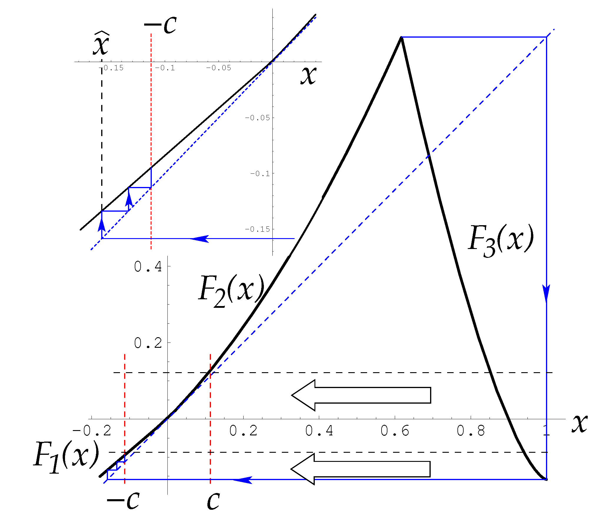
We highlight that ${\varphi }_{II}\left(x_n\right)$ considers only points coming from $F_3\left(x_{n-1}\right)$, where $x_n=F_3\left(x_{n-1}\right)$. Figure 12 shows the reinjection process governed by $F_1\left(x\right)$ and $F_3\left(x\right)$. In the larger figure, the evolution of the density generated by $F_3\left(x\right)$ is indicated with thick arrows and the red discontinuous lines show the laminar interval. In the smaller box, the evolution produced by $F_1\left(x\right)$ is shown with thin blue arrows. In this figure, a trajectory needs three iterations to move from $\widehat{x}$ to $x_0-c$.

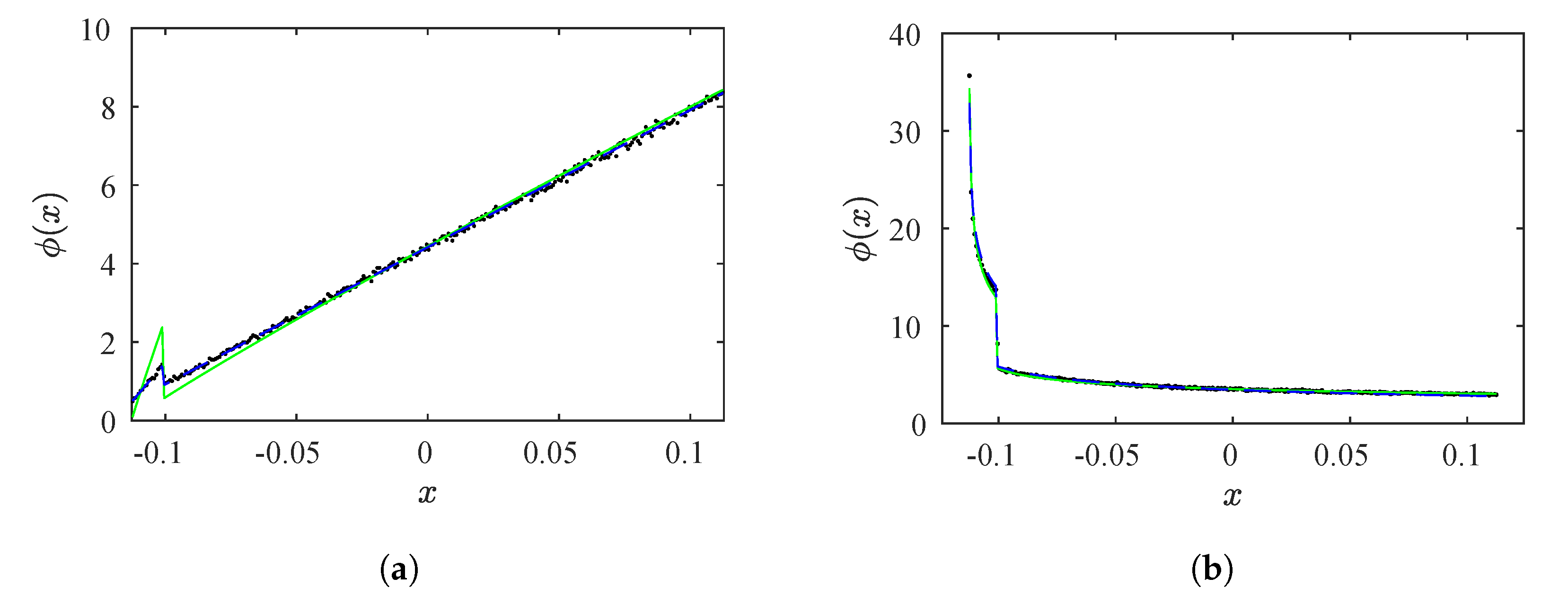
To validate the previous theoretical equations, we performed four sets of tests. The first one used $\epsilon =0.001$, $\gamma =0.5$, $y_m=1$, $x_0=0$, $c=0.1128$, $\widehat{x}=-0.158449931412894$, $N=1\times {10}^5-15\times {10}^5$, and $N_s=300$. For this set of tests, a trajectory took three iterations to displace from $\widehat{x}$ to $x_0-c$. We calculated the RPD function using the continuity technique, the M function methodology, and numerically. Figure 13a shows the comparison between the three RPDs. Black points are the numerical data, the green line is the RPD calculated using the M function methodology, and the RPD obtained by the continuity technique is the dashed blue line. We can observe that both methodologies, M function and continuity technique, capture the behavior of the numerical RPD. However, the continuity technique captures the numerical results more accurately. The rates of convergence using the continuity technique for $D_r$ and $E_r$ are $O\left(\frac{1}{N^{0.1}}\right)$ and $O\left(\frac{1}{N^{0.37}}\right)$, respectively. The values of $D_r$ and $E_r$ for $N=15\times {10}^5$ are $2.314\times {10}^{-3}$ and $1.426\times {10}^{-2}$, respectively.

The parameters for the second set of tests were the same but $\gamma =1.5$. Again, the trajectories took three iterations from $\widehat{x}$ to $x_0-c$. Results are shown in Figure 13b. Again, both methodologies capture the behavior of the numerical data. We have calculated the rates of convergence for the continuity technique: for $D_r$ it is approximately $O\left(\frac{1}{N^{0.06}}\right)$, and for $E_r$ is $O\left(\frac{1}{N^{0.15}}\right)$. For $N=15\times {10}^5$, we obtained $D_r=5.497\times {10}^{-3}$ and $E_r=3.925\times {10}^{-2}$.

The parameters for the third and fourth sets of tests were $\epsilon =0.001$, $y_m=1$, $x_0=0$, $c=0.1128$, $\widehat{x}=-0.12644444444$, $N=1\times {10}^5-15\times {10}^5$, and $N_s=300$. However, $\gamma =0.5$ for the third set of tests, and $\gamma =1.5$ for the fourth one. For both sets of tests, a trajectory needed only one iteration to move from $\widehat{x}$ to $x_0-c$. The theoretical and numerical results are shown in Figure 14a,b. The continuity technique and the M function methodology reproduce the behavior of the numerical RPD. However, from Figure 14a we can observe that the density technique approximates the numerical data more accurately. For the third set of tests, we have obtained $O\left(\frac{1}{N^{0.35}}\right)$ for $D_r$, and $E_r$, and for the fourth set of tests we have calculated $O\left(\frac{1}{N^{0.15}}\right)$ for $D_r$, and $E_r$.

The results of these four sets of tests are summarized in

Table 2. Results for the four tests. $p_e$ and $p_d$ are the order of convergence exponents for $E_r$, and $D_r$, respectively.

$\widehat{\mathit{x}}$	$\mathit{\gamma }$	${\mathit{p}}_{\mathit{e}}$	${\mathit{p}}_{\mathit{d}}$	${\mathit{E}}_{\mathit{r}}$	${\mathit{D}}_{\mathit{r}}$
$-0.158449931412894$	$0.5$	$0.37$	$0.10$	$1.426\times {10}^{-2}$	$2.314\times {10}^{-3}$
$-0.158449931412894$	$1.5$	$0.15$	$0.06$	$3.925\times {10}^{-2}$	$5.497\times {10}^{-3}$
$-0.12644444444$	$0.5$	$0.35$	$0.35$	$1.424\times {10}^{-2}$	$1.255\times {10}^{-3}$
$-0.12644444444$	$1.5$	$0.15$	$0.15$	$3.185\times {10}^{-2}$	$2.559\times {10}^{-3}$

. The first column is the lower boundary of reinjection $\widehat{x}$, the second one gives the exponent $\gamma$, the third and fourth columns are the order of convergence exponents for $E_r$ and $D_r$, respectively, and the last two columns show the calculated values of $E_r$ and $D_r$ for $N=15\times {10}^5$. We note that the rate of convergence and the values of $D_r$ and $E_r$ display a better behavior for $\gamma =0.5$ than for $\gamma =1.5$. This occurs mainly because for $\gamma =1.5$, the value of the numerical RPD in the first sub-interval is slightly larger than predicted by the continuity technique (see Figure 13a and Figure 14b).

From Figure 13 and Figure 14 and Table 2, we can notice that the theoretical evaluations obtained using the continuity technique and the M function methodology capture the numerical RPD behavior. In addition, we can observe that the continuity technique displays a better behavior than the M function methodology.

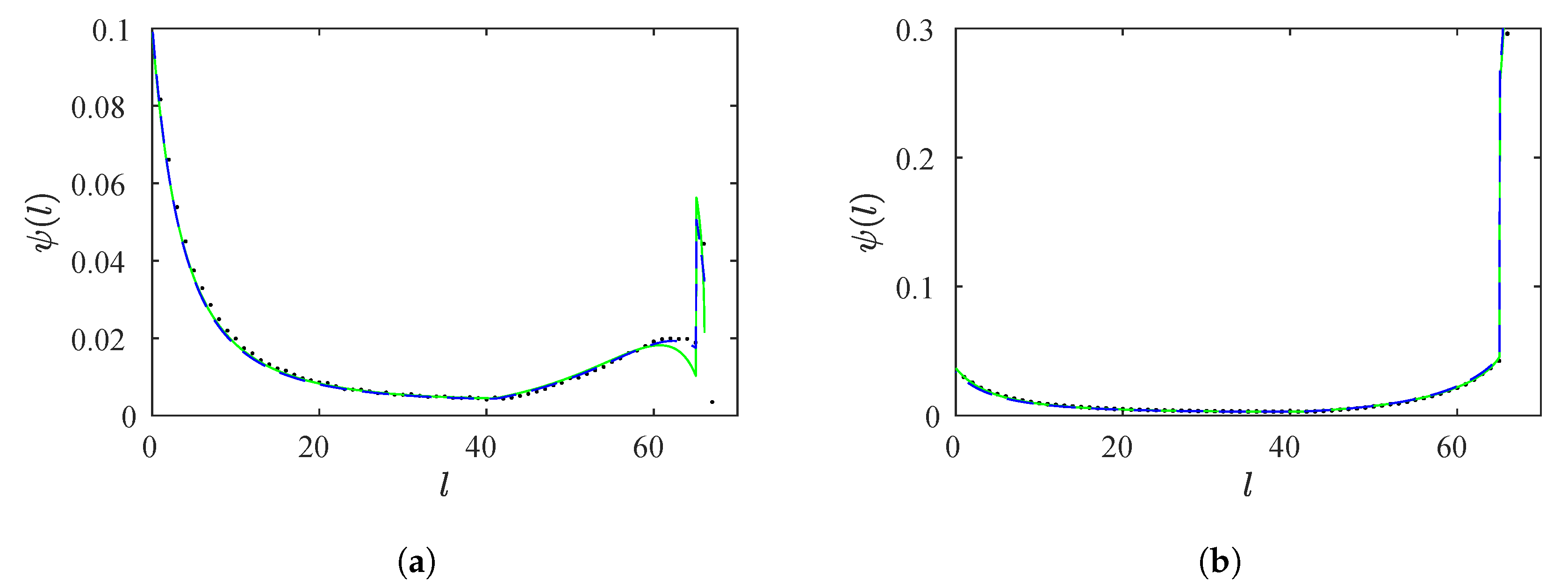
Probability Density of the Laminar Lengths

Once the RPD function is evaluated, we are able to calculate the probability density of the laminar lengths, $\psi \left(l\right)$, which determines the probability of finding laminar lengths between l and $l+dl$ [4]

$$\psi (l,c)=\varphi \left[X(l,c)\right]\left|\frac{dX(l,c)}{dl}\right|,$$

(53)

$X(l,c)$ is the inverse of $l(x,c)$, which is the laminar length for each reinjected point x. For the maps described by Equation (2), $\frac{dX(l,c)}{dl}$ is approximated by

$$\frac{dX(l,c)}{dl}=\left\{\begin{array}{cc}\epsilon +x({\lambda }_1-1)\hfill & x<0,\hfill \\ \epsilon +{\lambda }_2{x}^2\hfill & x\ge 0.\hfill \end{array}\right.$$

(54)

We calculated the RPDL functions for the four sets of tests previously presented. The results are shown in Figure 15 and Figure 16. We can observe a good accuracy between the continuity technique, the M function methodology, and the numerical data.

From Figure 13 and Figure 14, we can observe the different behaviors of the RPD functions. For $\gamma <1$, the number of trajectories that return close to the lower limit of the laminar interval is low, and the RPDs are increasing functions. For $\gamma >1$, the number of trajectories that return close to the lower limit of the laminar interval is high, and the RPDs are decreasing functions. These behaviors are also observed for the probability density of the laminar lengths (see Figure 15 and Figure 16). However, in all tests, we can observe two sub-intervals $[x_0-c,F_1(x_0-c))$ and $[F_1(x_0-c),x_0+c]$ with different behaviors described by Equation (36).

3. Conclusions

In this paper, we presented a new methodology to calculate the statistical properties of type V intermittency. This methodology is obtained from the evolution of densities (Perron–Frobenius operator), and we refer to it as the continuity technique. We introduced and utilized this technique to obtain the reinjection probability density function (RPD), $\varphi \left(x\right)$, and the probability density of the laminar lengths (RPDL), $\psi \left(l\right)$, for the family of maps described by Equation (2).

To the authors’ best knowledge, this is the first time that the continuity technique has been used to calculate the RPD and RPDL functions in type V intermittency. Furthermore, it is the first time that this technique is implemented where multiple iterations are needed to obtain the RPD and where the reinjection is generated simultaneously by two different processes.

We performed comparisons between the theoretical results obtained by the continuity technique with those calculated by the classical theory of intermittency, the M function methodology, and with numerical data. We found that both methodologies, continuity and M function, produce similar $\varphi \left(x\right)$ and $\psi \left(l\right)$ functions for different parameters, either with continuous or discontinuous RPD functions and with one or two functions governing the reinjection process. Furthermore, the theoretical results for the continuity technique accurately capture the numerical data. In addition, the results obtained with the continuity technique are more accurate than those calculated by the classical theory. We highlight that $\varphi \left(x\right)$ and $\psi \left(l\right)$ functions, calculated with the continuity technique, exhibit a wider range of behaviors than those expected by uniform reinjection.

The classical studies on type V intermittency use the assumption that the RPD is uniform [28,29,30]. More recent studies consider a less restrictive hypothesis of a constant density at pre-reinjection points, i.e., points that govern the reinjection process [26,27,35]. Here, the assumption of constant density at pre-reinjection points was analyzed for the family of maps described by Equation (2). The classic formulation of chaotic intermittency used a constant RPD. In this work, this condition was relaxed, allowing the RPD to be a more complex function. However, the hypothesis of constant density at pre-reinjection points was assumed. This assumption works accurately because the length of the laminar interval is small, and the RPD function depends, in addition to the density, on the derivative of the function at pre-reinjection points, which can take very large or close to zero values.

For continuous RPD functions, we have conducted several tests using different values of the exponent $\gamma$, the length of the laminar interval c, the parameter $\epsilon$, the number of reinjected points N, and the number of sub-intervals $N_s$. In all these tests for the continuity technique, the values of $D_r$ and $E_r$ decrease as the number of re-injected points grows, showing that the theoretical evaluation given by Equation (21) approximates the numerical RPD more accurately as the number of reinjected points increases. Furthermore, we have computed the rate of convergence of $D_r$ and $E_r$ for all tests, and detected that the process is convergent with a rate of convergence $O\left(\frac{1}{N^p}\right)$ within $0.35<p<0.5$. We emphasize that the continuity technique converges better than classical theory, and obtains RPDs with similar accuracy to the M function methodology.

A similar study was developed for discontinuous RPD functions using different values of $\gamma$ and the lower boundary of reinjection $\widehat{x}$. For all tests, we observe that the continuity technique captures the behavior of the numerical data. Furthermore, the RPDs calculated using the continuity technique are more accurate for several tests than those obtained with the M function methodology. For all tests performed with the continuity technique, $D_r$ and $E_r$ decrease as the number of re-injected points increases. The exponents to evaluate the order of convergence, $p_e$ and $p_d$ were always positive. In addition, the continuity technique has the advantage of allowing the prediction of analytic RPD functions, continuous or discontinuous, only knowing the map without the need for using numerical or experimental data. If the assumption of constant density at the pre-reinjection points can be used, the RPD function mainly depends on the map derivative at the pre-reinjection points (see Equation (13)).

We can conclude that the continuity technique has the ability to accurately calculate the RPD and RPDL functions for type V intermittency.