Abstract
The Lamé curve is an extension of an ellipse, the latter being a special case. Dr. Johan Gielis further extended the Lamé curve in the polar coordinate system by introducing additional parameters (n1, n2, n3; m): , which can be applied to model natural geometries. Here, r is the polar radius corresponding to the polar angle φ; A, B, n1, n2 and n3 are parameters to be estimated; m is the positive real number that determines the number of angles of the Gielis curve. Most prior studies on the Gielis equation focused mainly on its applications. However, the Gielis equation can also generate a large number of shapes that are rotationally symmetric and axisymmetric when A = B and n2 = n3, interrelated with the parameter m, with the parameters n1 and n2 determining the shapes of the curves. In this paper, we prove the relationship between m and the rotational symmetry and axial symmetry of the Gielis curve from a theoretical point of view with the condition A = B, n2 = n3. We also set n1 and n2 to take negative real numbers rather than only taking positive real numbers, then classify the curves based on extremal properties of r(φ) at φ = 0, π/m when n1 and n2 are in different intervals, and analyze how n1, n2 precisely affect the shapes of Gielis curves.
1. Introduction
Superellipses are defined by the equation:
where x and y represent the horizontal and vertical coordinates of points in the rectangular coordinate system, respectively; A, B and n are positive real numbers (n = +∞ is included). Superellipses include the circle, the diamond and the square for A = B, and the ellipse, the rhombus and the rectangle for A ≠ B [1,2]. Superellipses are a subgroup of Lamé curves whereby the absolute value signs ensure the symmetry of the shapes. The classic conic sections are special cases as well. In the most general cases, the exponent n can also be a negative real number [3].
Gielis [4,5] introduced more model parameters based on the superellipse equation in the polar coordinate system (see Equation (2) below), which extends superellipses to include various ranges of more symmetrical and asymmetrical geometries found in nature. The mathematical expression of the Gielis equation is as follows:
where r and φ are the polar radius and polar angle, respectively, and ni (i = 1, 2, 3) and m are positive real numbers.
For the past few years, various studies [6,7,8,9,10,11,12] have demonstrated the validity of the Gielis equation in describing actual biological geometries. The boundary coordinate data of leaves for 46 bamboo species [6], and eggs of 9 species of birds [7] were well fitted using the Gielis equation (m = 1); Tian et al. [8] used the Gielis equation (m = 2) to simulate the seed projections (in side view) of two Ginkgo biloba cultivars, which provided a fresh viewpoint to identify the morphological differences between species; Li et al. [9] compared the original Gielis equation (m = 3) with its twin version in describing the planar projections (in top view) of Koelreuteria paniculata fruits, and demonstrated that both the original and twin Gielis equation can describe the shapes of the vertical fruit projections well; Shi et al. [10,11] and Wang et al. [12] used the Gielis equation (m = 4, 5) to fit the outline shapes of tree-ring cross sections, sea stars and corolla tubes of Vinca major flowers, respectively, which further displayed various symmetric shapes with more angles generated by the Gielis equation. However, it seems that the above studies involving the Gielis equation were all application oriented, and the symmetry and periodicity of the equation were not studied systematically.
Gielis [4] pointed out that the values of ni (i = 1, 2, 3) and m have different roles for the formation of the shapes of curves generated by the Gielis equation. It is apparent that the unit circle (r = 1) is defined when n2 = n3 = 2 and A = B = 1. For n2 = n3 > 2, the shape circumscribes the unit circle, while the shape will inscribe in the unit circle for n2 = n3 < 2. The value of m determines the number of angles of the Gielis curves and the number of rotations which make the curve closed. The shapes will close after one rotation (0–2π) when m is a positive integer, in other words, . When m is positive but not an integer, the shapes will not close after one rotation (0–2π), that is, . When m is a positive rational number, the numerator of m determines the number of angles of the curves, and the denominator of m determines how many rotations the curves need to close. For example, when m = 4/3, the corresponding curves will close after three rotations (0–6π), generating four angles. The curves will never close if m is an irrational number.
Lenjou [13] proved that there were several invariants in the Gielis curves: the included area of the closed curves, the polar moment of inertia and the distance under angle φ = k/m (k ∈ ℝ), which are independent of the value of the positive integer m for the given values of ni (i = 1, 2, 3), A and B. However, it is not clear whether the proof can be upheld when the values of ni (i = 1, 2, 3) are negative and m is any rational number.
Matsuura [14] examined precisely and analytically the mathematical structure of Gielis curves from a theoretical point of view, analyzed the symmetry of Gielis curves with the condition A = B, and n2 = n3 and calculated the curvature at φ = π/m. This research was limited to the case of m ≥ 3, A = B, n2 = n3 and highlighted the role of m/4, since one could define Gielis polygons by choosing n1 = m2n2/16, in other words, when the ratio of . Under this condition, such polygons get closer to regular polygons for increasing m. Equation (2) also allows for describing regular polygons [15].
However, previous researches did not include the cases when the values of ni (i = 1, 2, 3) are negative. Gielis [5] shows the more general equation, to include negative values and the hyperbolic version with a minus sign between cosine and sine terms, and Spíchal [16] used negative values for approximating some flowers and leaves, but a systematic study is lacking. Here, we explore the rotational symmetry and axial symmetry of Gielis curves for the case of A = B, n2 = n3, and m is a rational number. In particular, we also analyze the influence of the parameters n1 and n2 which not only take positive real values, but can also be negative real numbers, on the shapes of Gielis curves.
2. Materials and Methods
We set A = B, n2 = n3 in Equation (2) so that we have:
where . For n2 = 2, a circle of radius a is obtained. Here, n1, n2 are real numbers and n1 ≠ 0, which determine the shapes of the Gielis curves, and m is a rational number, which determines the number of angles for a closed curve.
We will discuss the symmetry and periodicity of r(φ) in Equation (3) in the form of formulas. Since , which results in the role of the sign of m to r(φ) in Equation (3) being hidden by the absolute value sign, that is , we just need to consider the case of m > 0. Setting m = p/q (p and q are positive integers that are coprime numbers), we have:
Equation (4) indicates that r(φ) in Equation (3) is a periodic function with T1 = 2qπ, where T1 is the minimum closure period. In particular, r(0) = r(2qπ), which manifests that Gielis curves generated by Equation (3) start from φ = 0, close firstly after q rotations, and this pattern will be repeated every 2qπ that we call the minimum closure period. Therefore, we just need to investigate the characters of the curves at .
Additionally, when we set in Equation (3), it follows that
Equation (5) indicates that r(φ) in Equation (3) is also a periodic function with T2 = 2π/m, which shows that Gielis curves generated by Equation (3) are rotationally symmetric with rotation angle 2π/m. We call T2 the minimum rotation period when . In particular, the minimum closure period (T1) divided by the minimum rotation period (T2) is equal to p, that is: (m = p/q), which suggests that each angle corresponds to a minimum rotation period and the curves generate p angles in a minimum closure period.
The above analysis indicates that the shapes generated by Equation (3) have a rotational symmetry and the rotation angle is equal to 2π/m when . Shapes then are always repeated for each 2π/m. So, we just need to consider the curves with , and the axial symmetry of the shapes on this interval is shown as follows:
which indicates that Gielis curves generated by Equation (3) are axisymmetric about the line y = tan(π/m)x when .
The invariants of supershape generated by Equation (3), area, polar moment of inertia and distance under angle φ = k/m (k ∈ ℝ) [13] will be reconsidered as follows when n1, n2 are real numbers, and m is a rational number. Considering the integral A:
Equation (7) indicates that the integral A is independent of the numerator of m. When the denominator of m is equal to 1, that is, m is a positive integer, the integral A represents the area of the closed Gielis curves, which is an invariant for the given values of the parameters n1, n2, a. However, the integral A is not the area when the denominator of m is not equal to 1, the reason being that the area of the closed Gielis curves is doubly-counted many times in this case. It is worth noting that the integral A is not always convergent. We can conclude that when n1, n2 are both negative, the integral A is convergent with , while A is divergent with ; while the integral A is always convergent when at least one of the parameters n1 and n2 is positive.
The discussion about the polar moment of inertia is similar to the area. Considering the integral I:
Equation (8) manifests that the integral I is independent of the numerator of m. When q, the denominator of m, is equal to 1, the integral I represents the polar moment of inertia of the supershape, which is an invariant for the given values of the parameters n1, n2, a. Similarly, the integral I is always convergent when at least one of the parameters n1 and n2 is positive, while when n1, n2 are both negative, the integral I is convergent with , and A is divergent with .
When φ = k/m, we have:
where k is any real number. Equation (9) means that the distance under angle φ = k/m is independent of the value of m with any real numbers n1, n2, and any rational number m.
We now discuss the variations of Gielis curves based on the characteristics of extreme points of the polar coordinates equation r(φ) in Equation (3). For , the first derivative of r(φ) in Equation (3) can be calculated as:
where d represents differential notation. Setting we have:
which indicates that r(φ) may reach its extreme value at φ = π/m, 0 for n2 > 1, and φ = π/m for n2 ≤ 1 with . Since φ = π/m may always be an extreme point, we give priority to the characteristics of the curves at that point. For φ = π/m, the second derivative of r(φ) in Equation (3) can be calculated as:
The sign of the second derivative is used to study whether the equation r(φ) reaches a maximal value or a minimal value at a certain point. Apparently, the sign of in Equation (12) is determined by , and we have:
Equation (13) indicates that r(φ) in Equation (3) will reach its maximal value at φ = π/m when or , and will reach its minimal value at φ = π/m when or . Similarly, we calculate the second derivative of r(φ) at φ = 0 with the condition n2 > 1:
Equation (14) indicates that the sign of the second derivative of r(φ) at φ = 0 is determined by n2/n1 when n2 > 1. For 1 < n2 < 2, when n1 and n2 have the same sign, which means that r(φ) in Equation (3) will reach its maximal value at φ = 0; and when n1 and n2 have the opposite sign, which means that r(φ) will reach its minimal value at φ = 0. For n2 > 2, when n1 and n2 have the same sign, which means that r(φ) in Equation (3) will reach its minimal value at φ = 0; and when n1 and n2 have the opposite sign, which means that r(φ) will reach its maximal value at φ = 0. While for n2 = 2, since r(φ) = a, which represents a circle of radius a.
All calculations and figures were accomplished by using the statistical software R (version 4.2.0) [17] with the ‘biogeom’ package (version 1.0.8) [18].
3. Results
Graphs are used to explain the rotational symmetry and axial symmetry of Gielis curves. An example of Gielis curves with parameter m taking a positive integer, and a positive rational number but not an integer, is shown in Figure 1. The various cases which are obtained from different values of n1 and n2 in Equation (13) will be discussed in the following paragraphs (m = 5 in each case).
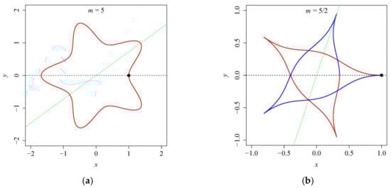
Figure 1.
Representative curves generated by Equation (3) with a = 1, n1 = 2, n2 = 5, m = 5 (a) and with a = 1, n1 = 0.5, n2 = 0.5, m = 5/2 (b). (a) Gielis curve (red line) with 5 angles closes after one rotation (0–2π) for m = 5, which is rotationally symmetric with rotation angle 2π/5; the green line is the axis of symmetry y = tan(π/5)x; (b) Gielis curve (red line and blue line represent the curve generated by r(φ) when φ ∈ [0, 2π) and [2π, 4π), respectively) with 5 angles closes after two rotations (0–4π) for m = 5/2, which is rotationally symmetric with rotation angle 4π/5; the green line is the axis of symmetry y = tan(2π/5)x.
- n1 > 0, n2 > 2;
r(φ) has two extreme points (φ = 0, π/m) and when n1 > 0, n2 > 2, which indicates that r(φ) in Equation (3) reaches its maximal value at φ = π/m and its minimal value at φ = 0. Figure 2 shows the corresponding Gielis curves in this situation, which manifests that all of the curves are circumscribed on the circle (r = a). In addition, the curves are fuller with increasing n1; this change makes the differentiated degree of angles of Gielis curves decrease gradually. The parameter n2 affects the steepness of the corners to some extent, that is, the rmax values of the curves increase as n2 increases, making the curves become more bent. The corners of Gielis curves are rounded by a small value of n2 (Figure 2) and are sharpened by a large value of n2 (Figure A1b). Special cases occur when the shape is a series of lines radiating from the center (Figure A1a) when n1 is small enough and n2 is large enough, and the shape will be like a circle (Figure A1c) when n1 is large enough and n2 is small enough.
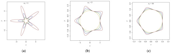
Figure 2.
Gielis curves generated by Equation (3) for a = 1, m = 5. The values of n1 are 1 (a), 5 (b), 10 (c), respectively, and the values of n2 are 2, 4, 6, 8 from the inside out in each panel.
- n1 > 0, n2 < 0;
r(φ) has only one extreme point (φ = π/m) and when n1 > 0, n2 < 0, which indicates that r(φ) reaches its maximal value at φ = π/m. Figure 3 shows the corresponding Gielis curves in this situation, which indicate that when n1 increases, the curves become fuller. Further, when n2 increases, the values of rmax of the curves increase, making the corners rounded. In addition, the shape recedes inward into lines (Figure A2a) when n1 and n2 are small enough, while the shape expands outward into a circle (Figure A2c) when n1 and n2 are large enough. A special case occurs when the curve turns into a circle () with n2 = 0.
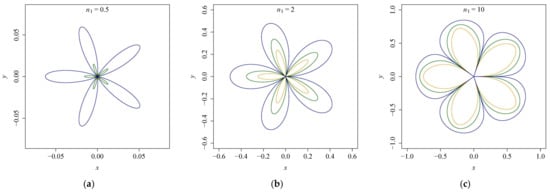
Figure 3.
Gielis curves generated by Equation (3) for a = 1, m = 5. The values of n1 are 0.5 (a), 2 (b), 10 (c), respectively, and the values of n2 are −6, −4, −2 from the inside out in each panel.
- n1 < 0, 0 < n2 < 2;
r(φ) has only one extreme point (φ = π/m) and when n1 < 0, 0 < n2 ≤ 1, which indicates that r(φ) reaches its maximal value at φ = π/m; in contrast, r(φ) has two extreme points (φ = 0, π/m) and when n1 < 0, 1 < n2 < 2, which indicates that r(φ) reaches its minimal value at φ = 0 and its maximal value at φ = π/m. Figure 4 shows the corresponding Gielis curves in this situation, from which it can be seen that the curves will be fuller as n1 decreases from 0 to −∞, with rmax values of the curves decreasing as n2 increases. In addition, the curves at φ = 0 are sharpened when 0 < n2 ≤ 1, and are flattened when 1 < n2 < 2. Special cases occur when the shape expands outward into a circle () and shrinks inward into a circle (r = a) with n2 = 0 and 2, respectively.
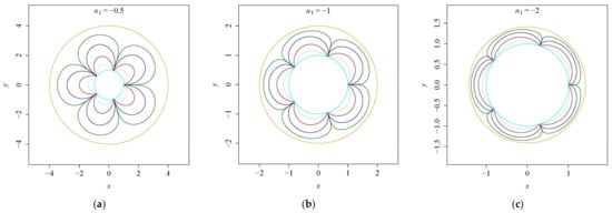
Figure 4.
Gielis curves generated by Equation (3) for a = 1, m = 5. The values of n1 are −0.5 (a), −1 (b), −2 (c), respectively, and the values of n2 from the outside in are 0, 0.2, 0.5, 1, 1.5, 2 in each panel.
- n1 > 0, 0 < n2 < 2;
r(φ) has only one extreme point (φ = π/m) and when n1 > 0, 0 < n2 ≤ 1, which indicates that r(φ) reaches its minimal value at φ = π/m; while r(φ) has two extreme points (φ = 0, π/m) and when n1 > 0, 1 < n2 < 2, which indicates that r(φ) reaches its maximal value at φ = 0 and its minimal value at φ = π/m. Figure 5 shows the corresponding Gielis curves in this situation, similarly to the case of n1 < 0, 0 < n2 < 2, where the curves are fuller as n1 increases from 0 to +∞, and the values of rmin increase as n2 increases. Additionally, the curves at φ = 0 are sharpened with 0 < n2 ≤ 1, and are flattened with 1 < n2 < 2. Special cases occur when the shape shrinks inward into a circle () and expands outward into a circle (r = a) with n2 = 0 and 2, respectively.
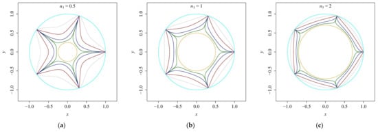
Figure 5.
Gielis curves generated by Equation (3) for a = 1, m = 5. The values of n1 are 0.5 (a), 1 (b), 2 (c), respectively, and the values of n2 are 0, 0.2, 0.5, 1, 1.5, 2 from the inside out in each panel.
- n1 < 0, n2 > 2;
r(φ) has two extreme points (φ = 0, π/m) and when n1 < 0, n2 > 2, which indicates that r(φ) reaches its maximal value at φ =0 and its minimal value at φ = π/m. Figure 6 shows the corresponding Gielis curves in this situation, where all of the curves are inscribed in the circle (r = a). Contrary to the case of n1 > 0, n2 > 2, the curves turn fuller with decreasing n1, and rmin values of the curves decrease (even to zero) as n2 increases, making the curves more bent. Special cases occur when the shape is similar to a series of radiating lines (Figure A3a) when both n1 and n2 are large enough, and the shape will be similar to a circle (Figure A3c) when both n1 and n2 are small enough.
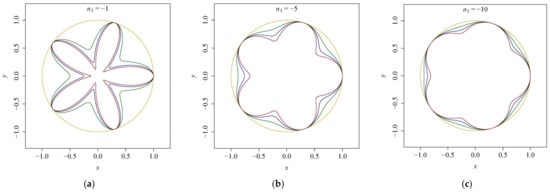
Figure 6.
Gielis curves generated by Equation (3) for a = 1, m = 5. The values of n1 are −1 (a), −5 (b), −10 (c), respectively, and the values of n2 from the outside in are 2, 4, 6, 8 in each panel.
- n1 < 0, n2 < 0.
r(φ) has only one extreme point (φ = π/m) and when n1 < 0, n2 < 0, which indicates that r(φ) reaches its minimal value at φ = π/m. Figure 7 shows the corresponding Gielis curves in this situation, where the curves become fuller with decreasing values of n1, and the rmin values of the curves decrease as n2 increases. Noteworthy is that r(φ) is not always continuous as r(0) = +∞, which means that the curves are not closed under this circumstance.
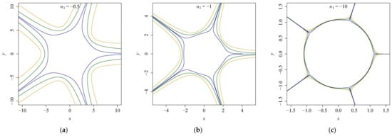
Figure 7.
Gielis curves generated by Equation (3) for a = 1, m = 5. The values of n1 are −0.5 (a), −1 (b), −10 (c), respectively, and the values of n2 from the outside in are −0.6, −0.4, −0.2 in each panel.
4. Discussion and Conclusions
As a generalization of Lamé curves, in particular superellipses, Equation (2) with its six parameters can generate various natural geometries providing a six dimensional manifold or catalogue of shapes. We have a powerful representation with fewer parameters, as in Equation (3) with A = B and n2 = n3, which diminishes the possibility of generating an asymmetrical shape. The present work is a necessary step in the future for the applied investigation of concave shapes, and the notion of invariants, which is exactly reflected by examining the influence of negative exponents on geometries, is crucial for any studies pertaining to natural shapes and phenomena. However, natural biological geometries are more or less influenced by abiotic and biotic factors, which lead them to exhibit a certain asymmetry [19,20,21]. Such a phenomenon is usually referred to as fluctuating asymmetry [22,23]. The ‘biogeom’ package [18] based on R (version ≥ 4.2.0) [17] is a readily-available tool for fitting actual boundary coordinate data of natural shapes following Equation (3), and the fluctuating asymmetry that has been found in nature, especially the leaves of garden plants [24], can be quantified by the prediction error of data fitting.
Equation (3) displays a mathematical expression for natural geometries at an ideal state without being influenced by environmental stress. Nevertheless, it is necessary to make a symmetrical hypothesis to quantify the extent of deviation from perfectly symmetrical geometries. In this study, we discussed the relationship of the parameter m (a rational number) with symmetry of curves generated by Equation (3), investigated the invariants (area, polar moment of inertia and distance under angle φ = k/m) when n1, n2 are negative and m is a rational number and explored how the parameters n1, n2 control the shapes of the curves. For any m = p/q, the denominator q determines how many rotation curves are needed for the figure to close, and the numerator p determines the number of angles for a closed curve. Additionally, the shapes generated by Equation (3) are rotationally symmetric and axisymmetric, and m determines the rotation angle and the position of the axis of symmetry.
It is noted that the meanings of invariants have changed since the integrals do not always represent area or polar moment of inertia for a closed Gielis curve when m is any rational number, and the integrals may diverge with negative numbers n1, n2. On the other hand, the parameters n1 and n2 determine the shapes of the Gielis curves, which have different influences on the curves. The shapes tend to be fuller when the absolute value of n1 increases, and when the absolute value of n2 increases, the curves at φ = (2t + 1)π/m (t ∈ ℕ) become less flattened with n2 < 0 or n2 > 2, where r(φ) can take the maximal (or minimal) value. We can see that curves of various shapes are obtained when the absolute values of n1 and n2 are both large enough (Figure A1b, Figure A2b and Figure A3b). The shapes can be circles (Figure 4 and Figure 5) with n2 = 0 or 2, which indicates that the shapes tend to be circular whether n2 increases or decreases with 0 < n2 < 2. However, the shapes can be radiating lines or circles (Figure A1, Figure A2 and Figure A3) with n2 < 0 or n2 > 2 when the values of n1, n2 are large or small enough, which represents a limiting case of Gielis curves. In addition, whether r(φ) can reach its maximal or minimal value at φ = (2t + 1)π/m (t ∈ ℕ) determines the location of the corners. The corners of Gielis curves lie at φ = (2t + 1)π/m (t ∈ ℕ) if the points are maximal value points of r(φ), while the corners lie at φ = 2tπ/m (t ∈ ℕ) if the points are minimal value points.
Different from most previous research, we studied the cases when m takes any rational number, and n1, n2 not only can take positive real numbers, but also negative real numbers. This opens up a new catalogue of shapes and geometries. In this work, we focused on the extremal property of the points (φ = 2tπ/m and (2t + 1)π/m, t ∈ ℕ) of r(φ) in Equation (3), and classified the curves based on various combinations of the values of n1 and n2, which can provide guidance for applying the Gielis equation to simulate the shapes of natural biology. However, the geometries of biological organs and issues are not perfectly axisymmetric or rotationally symmetric. Natural shapes are always asymmetrical, which result from several abiotic and biotic factors, including radiation, temperature, nutrient supply and physical pressure between individuals. We first need to build symmetric models for describing natural shapes in biology, and then we can quantify these factors, which can generate asymmetric geometries in the models to render the refined models to be more powerful in describing natural geometries. Therefore, the present work might be a necessary step in studying the fluctuating asymmetry in evolutionary biology. Future research on the geometries extended from symmetry to asymmetry in this study area is worthwhile because it can provide insights into the fluctuating asymmetry of natural geometries.
Author Contributions
Investigation, L.W.; formal analysis, L.W. and J.G.; writing—original draft preparation, L.W.; writing—review and editing, D.A.R., P.E.R. and P.S.; supervision, J.G. and P.S. All authors have read and agreed to the published version of the manuscript.
Funding
This research received no external funding.
Data Availability Statement
Not applicable.
Acknowledgments
The authors would like to thank Weijia Hou and Qi Zhang for their valuable support and encouragement.
Conflicts of Interest
The authors declare no conflict of interest.
Appendix A
Several Figures cited in the main text.

Figure A1.
Gielis curves generated by Equation (3) for a = 1, m = 5. (a) n1 = 1, n2 = 1000; (b) n1 = 1000, n2 = 1000; (c) n1 = 1000, n2 = 3.

Figure A2.
Gielis curves generated by Equation (3) for a = 1, m = 5. (a) n1 = 1, n2 = −1000; (b) n1 = 1000, n2 = −1000; (c) n1 = 1000, n2 = −1.

Figure A3.
Gielis curves generated by Equation (3) for a = 1, m = 5. (a) n1 = −1, n2 = 10,000; (b) n1 = −10,000, n2 = 10,000; (c) n1 = −10,000, n2 = 3.
References
- Lamé, G. Examen des Différentes Méthodes Employées Pour Résoudre les Problèmes de Géométrie; V. Courcier: Paris, France, 1818. [Google Scholar]
- Gridgeman, N.T. Lamé ovals. Math. Gaz. 1970, 54, 31–37. [Google Scholar] [CrossRef]
- Jaklič, A.; Leonardis, A.; Solina, F. Segmentation and Recovery of Superquadrics; Kluwer Academic Publishers: Dordrecht, The Netherlands, 2000. [Google Scholar]
- Gielis, J. A general geometric transformation that unifies a wide range of natural and abstract shapes. Am. J. Bot. 2003, 90, 333–338. [Google Scholar] [CrossRef]
- Gielis, J. The Geometrical Beauty of Plants; Atlantis Press: Paris, France, 2017. [Google Scholar]
- Lin, S.; Zhang, L.; Reddy, G.V.P.; Hui, C.; Gielis, J.; Ding, Y.; Shi, P. A geometrical model for testing bilateral symmetry of bamboo leaf with a simplified Gielis equation. Ecol. Evol. 2016, 6, 6798–6806. [Google Scholar] [CrossRef] [PubMed]
- Shi, P.; Gielis, J.; Niklas, K.J. Comparison of a universal (but complex) model for avian egg shape with a simpler model. Ann. N. Y. Acad. Sci. 2022, 1514, 34–42. [Google Scholar] [CrossRef] [PubMed]
- Tian, F.; Wang, Y.; Sandhu, H.S.; Gielis, J.; Shi, P. Comparison of seed morphology of two ginkgo cultivars. J. For. Res. 2020, 31, 751–758. [Google Scholar] [CrossRef]
- Li, Y.; Quinn, B.K.; Gielis, J.; Li, Y.; Shi, P. Evidence that supertriangles exist in nature from the vertical projections of Koelreuteria paniculata fruit. Symmetry 2022, 14, 23. [Google Scholar] [CrossRef]
- Shi, P.; Huang, J.; Hui, C.; Grissino-Mayer, H.D.; Tardif, J.C.; Zhai, L.; Wang, F.; Li, B. Capturing spiral radial growth of conifers using the superellipse to model tree-ring geometric shape. Front. Plant Sci. 2015, 6, 856. [Google Scholar] [CrossRef] [PubMed]
- Shi, P.; Ratkowsky, D.A.; Gielis, J. The generalized Gielis geometric equation and its application. Symmetry 2020, 12, 645. [Google Scholar] [CrossRef]
- Wang, L.; Miao, Q.; Niinemets, Ü.; Gielis, J.; Shi, P. Quantifying the variation in the geometries of the outer rims of corolla tubes of Vinca major L. Plants 2022, 11, 1987. [Google Scholar] [CrossRef] [PubMed]
- Lenjou, K. Krommen en Oppervlakken van Lamé en Gielis: Van de Formule van Pythagoras tot de Superformule. Master’s Thesis, University of Louvain, Brussels, Belgium, 2005. [Google Scholar]
- Matsuura, M. Gielis’ superformula and regular polygons. J. Geom. 2015, 106, 383–403. [Google Scholar] [CrossRef]
- Ricci, P.E.; Gielis, J. From Pythagoras to Fourier and from Geometry to Nature; Athena International Publishing: Amsterdam, The Netherlands, 2022. [Google Scholar]
- Spíchal, L. Superelipsa a superformule. Mat.–Fyzika–Inform. 2020, 29, 54–69. [Google Scholar]
- R Core Team. R: A Language and Environment for Statistical Computing; R Foundation for Statistical Computing: Vienna, Austria, 2022; Available online: https://www.R-project.org/ (accessed on 1 June 2022).
- Shi, P.; Gielis, J.; Quinn, B.K.; Niklas, K.J.; Ratkowsky, D.A.; Schrader, J.; Ruan, H.; Wang, L.; Niinemets, Ü. ‘biogeom’: An R package for simulating and fitting natural shapes. Ann. N. Y. Acad. Sci. 2022, 1516, 123–134. [Google Scholar] [CrossRef] [PubMed]
- Tucić, B.; Miljković, D. Fluctuating asymmetry of floral organ traits in natural populations of Iris pumila from contrasting light habitats. Plant Species Biol. 2010, 25, 173–184. [Google Scholar] [CrossRef]
- Klisarić, N.B.; Miljković, D.; Avramov, S.; Zivković, U.; Tarasjev, A. Fluctuating asymmetry in Robinia pseudoacacia leaves—Possible in situ biomarker? Environ. Sci. Pollut. Res. Int. 2014, 21, 12928–12940. [Google Scholar] [CrossRef]
- Miljković, D.; Stefanović, M.; Orlović, S.; Stanković Neđić, M.; Kesić, L.; Stojnić, S. Wild cherry (Prunus avium (L.)) leaf shape and size variations in natural populations at different elevations. Alp. Bot. 2019, 129, 163–174. [Google Scholar] [CrossRef]
- Palmer, A.R. Fluctuating asymmetry analyses: A primer. In Proceedings of the International Conference on Developmental Instability: Its Origins and Evolutionary Implications, Tempe, Arizona, USA, 14–15 June 1993; Markow, T.A., Ed.; Springer: Dordrecht, The Netherlands, 1994; pp. 335–364. [Google Scholar]
- Palmer, A.R.; Strobeck, C. Fluctuating asymmetry: Measurement, analysis, patterns. Ann. Rev. Ecol. Syst. 1986, 17, 391–421. [Google Scholar] [CrossRef]
- Wang, C.; Guo, M.; Jin, J.; Yang, Y.; Ren, Y.; Wang, Y.; Cao, J. Does the Spatial Pattern of Plants and Green Space Affect Air Pollutant Concentrations? Evidence from 37 Garden Cities in China. Plants 2022, 11, 2847. [Google Scholar] [PubMed]
Publisher’s Note: MDPI stays neutral with regard to jurisdictional claims in published maps and institutional affiliations. |
© 2022 by the authors. Licensee MDPI, Basel, Switzerland. This article is an open access article distributed under the terms and conditions of the Creative Commons Attribution (CC BY) license (https://creativecommons.org/licenses/by/4.0/).