A New Symbolic Time Series Analysis Method Based on Time-to-Space Mapping, through a Symmetric Magnetic Field, Quantized by Prime Numbers

Abstract

This work presents a new analysis method for two-symbol symbolic time series based on the time-to-space mapping achieved through a device of current carrying circular rings. An algorithm based on the theory of prime numbers is proposed for the approximate estimation of the stratified magnetic field produced by the aforementioned device. The main property of the specific algorithm is that it quantizes the stratified magnetic field. If a two-symbol symbolic time series is used to determine the flow directions of the rings’ currents, a time-to-space mapping of the dynamics of the system producing the time series is observed. A unique “fingerprint” of the symbolic dynamics is shaped by the spatial allocation of the values of the six-valued symmetric quantized magnetic field produced by the device. This allows for the quantitative evaluation of the original system’s dynamics by analyzing the resultant quantized magnetic field values space allocation, in a spectrum ranging from the lack of dynamics (randomness) to the presence of dynamics at all scales (criticality). Two examples of application–corresponding to the extremes of the dynamics spectrum, specifically, for symbolic time series resulting from (a) a random numbers generator and (b) the spin alternation of 2D-Ising in its critical state, verify the reliable time-to-space mapping of the involved symbolic dynamics. Moreover, an application to the symbolic sequence produced by the DNA of the GAPDH (Glyceraldehyde-3-Phosphate Dehydrogenase) human gene is presented as a real-world, intermediate dynamics case. The proposed symbolic time series analysis method presents the advantage that can take into account information related to both symbols, which is particularly useful in analyzing two-symbol time series of relatively short length where the probabilities of occurrence of the two symbols are not equal. By inferring the universality class of an artificial-neural-network-based hybrid spin model through the value of the critical exponent $\delta$, it is shown that for such time series, the proposed method provides a unique way to expose the real dynamics of the underlying complex system, in contrast to the analysis of waiting times in the time domain that leads to an ambiguous quantitative result.

1. Introduction

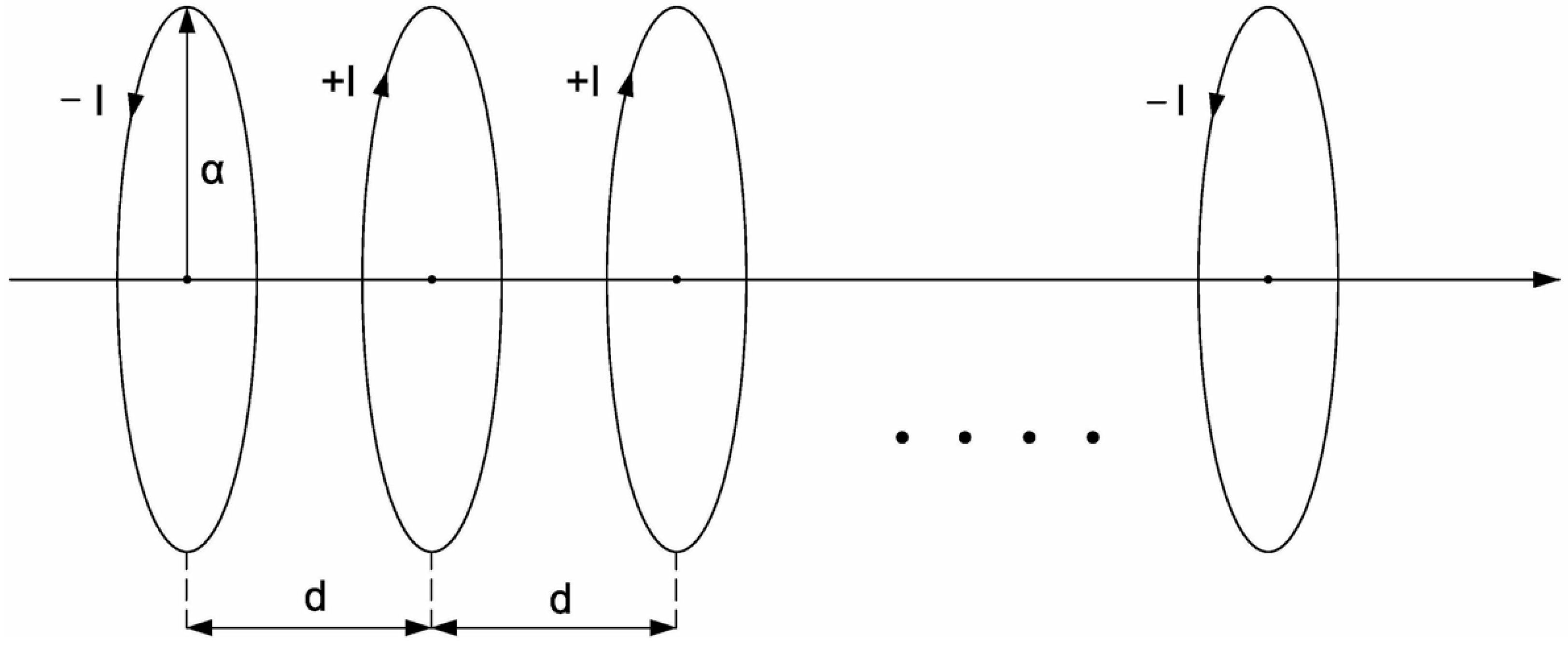
In the works [1,2], a device of identical current carrying circular rings (shown in Figure 1) has been studied, through which electric currents of the same intensity $I$ flow, but their flow direction ($+I,-I$) is randomly chosen, with equal probability.

Assuming that the number of rings is $N$, then the magnetic field at the center of the $k$-th ring $\left(k=1,2,\dots , N\right)$ is of the following form [2]:

$$B_k=\frac{1}{2}{\alpha }^2{d}^{-3}I\left\{{{\displaystyle \sum }}_{n=0}^{k-1}\frac{I_{k-n}}{{\left(n^2+c^2\right)}^{3/2}}+{{\displaystyle \sum }}_{n=0}^{N-k-1}\frac{I_{n+1+k}}{{\left[{\left(n+1\right)}^2+c^2\right]}^{3/2}}\right\},$$

(1)

where $\alpha$ is the radius of the rings, $d$ is the distance between two consecutive rings, $c=a/d$ and in each ring flows a current of intensity ${\rm I}$ and direction, $I_{k-n}$, $I_{n+1+k}$, described by a dichotomic variable taking the values $+1,-1$. The two sums appearing in the curly brackets of Equation (1) can respectively be written as:

$${{\displaystyle \sum }}_{n=0}^{k-1}\frac{I_{k-n}}{{\left(n^2+c^2\right)}^{3/2}}=\frac{I_k}{c^3}+{{\displaystyle \sum }}_{n=1}^{k-1}\frac{I_{k-n}}{{\left(n^2+c^2\right)}^{3/2}}$$

(2)

and

$${{\displaystyle \sum }}_{n=0}^{N-k-1}\frac{I_{n+1+k}}{{\left[{\left(n+1\right)}^2+c^2\right]}^{3/2}}={{\displaystyle \sum }}_{m=1}^{N-k}\frac{I_{m+k}}{{\left[m^2+c^2\right]}^{3/2}},$$

(3)

where $m=n+1$.

Substituting Equations (2) and (3) in Equation (1) one gets:

$$B_k=\frac{1}{2}{\alpha }^2{d}^{-3}I\left\{\frac{I_k}{c^3}+{{\displaystyle \sum }}_{n=1}^{k-1}\frac{I_{k-n}}{{\left(n^2+c^2\right)}^{3/2}}+{{\displaystyle \sum }}_{m=1}^{N-k}\frac{I_{m+k}}{{\left[m^2+c^2\right]}^{3/2}}\right\}.$$

(4)

Equation (4) can be seen as a “physics-based algorithm” (PA) based on the Biot-Savart law that calculates the magnetic field $B_k$ at all positions $k$ of the device’s axis. As it has been shown in [1,2], the magnetic field inside the device is interesting when $c<1$. In this case, for directions of currents determined by a dichotomic variable taking the values $+1,-1$ with equal probability, a stratification of the values of the magnetic field appears characterized by the existence of empty regions (cancelation) and zones where the fluctuations dominate (see Figure 2a in Section 2).

Symbolic dynamics refers to a description of complex systems, according to which a complex system is considered as an information generator producing messages consisting of a discrete set of symbols defined by partitioning the full continuous phase space into a finite number of cells, thus implementing a coarse graining strategy. The simplest possible coarse graining corresponds to the assignment of just two symbols “0” and “1”, or “$-1$” and “$+1$”, etc., to the original time series, depending on whether the time series original value is above or below a specific threshold (binary partition). On the other hand, some physical or numerical systems are inherently described in terms of discrete states, e.g., spin systems or DNA sequences, and thus we can say that these innately fit the description of the symbolic dynamics.

Let us consider a two-symbol symbolic time series $\left\{x\left(t_i\right)\right\}$, $t_i=i·\tau$, $\tau$ being the sampling period and $i=1,2,\dots , N$, with $x\left(t_i\right)$ taking the (symbol) values “$-1$” and “$+1$”. The “introduction” of such a two-symbol symbolic time series into the device of current carrying circular rings of Figure 1 can be achieved by mapping the chronological order of the symbols of the symbolic time series to the positions $k$ of the rings, while the symbol of each specific time point is used to determine the flow direction of the ring’s current at the corresponding position. Namely, the sequence of currents of the device, and specifically their flow direction, is determined by the corresponding time series symbol in such way that the symbol of $x\left(t_1\right)$ determines the current flow direction $I_1$ of the ring at the position $k=1$, the symbol of $x\left(t_2\right)$ determines the current flow direction $I_2$ of the ring at $k=2,$ and so on. For example, for $i=k=1$, if $x\left(t_1\right)=-1$, then $I_1=-1$, while if $x\left(t_1\right)=+1$, then $I_1=+1$, etc.

In the present work, we first investigate whether such an “introduction” of a two-symbol symbolic time series–that is produced directly or indirectly (after coarse graining) by a dynamic system–into the device of Figure 1 could be seen as a “transformation” from the time domain to the space domain, through which the dynamics of the system producing the time series can be carried over to the magnetic field produced by the device of Figure 1. Specifically, it is investigated whether the spatial allocation of the values of such a magnetic field can be considered as a “fingerprint” of the dynamics of the system that produces the symbolic time series, which can provide information about the evaluation of system’s dynamics, and thus constitutes a time-to-space mapping of symbolic dynamics. In such a case, it should be able to identify the dynamic behaviors in a spectrum that extends from the complete absence of dynamics, where the successive values of the time series are completely uncorrelated to each other, to the presence of dynamics at all scales–as happens in critical dynamics, where correlations appear in all space-time scales. As it is shown in the following, this is accomplished after the discretization (“quantization”) of the stratified magnetic field of the device of Figure 1 that is successfully verified by a prime-numbers-based algorithm for the approximate estimation of the magnetic field.

Inspired by the time domain analysis of complex systems’ time series that is based on the study of waiting times distribution, we propose a space domain analysis of two-symbol symbolic time series that is based on the study of the spatial allocation of the values of the six-valued symmetric quantized magnetic field produced by the device when the sequence of currents’ flow direction is determined by the time series symbols.

It is shown that although the existence of dynamics in two-symbol symbolic time series can be revealed in the time domain by the scaling behavior of waiting times, the quantitative result is ambiguous; the involved exponent cannot be definitely determined since the exponent’s value depends on the considered symbol. The proposed analysis in the space domain, and specifically by taking into account the dynamics of both symbols of the original symbolic time series, provides a solution to this problem. It provides a unique way to expose the real dynamics of a complex system for which a relatively short time series is available and the probabilities of occurrence of the two symbols are not equal. As an example, demonstrating the usefulness of the proposed symbolic time series analysis method, the universality class of an artificial-neural-network-based hybrid spin model is successfully inferred through by value of the critical exponent $\delta$, while for the same example it is shown that the analysis in the time domain, i.e., by means of waiting times, leads to an ambiguous quantitative result.

2. The Application of the Physics-Based Algorithm to Symbolic Dynamics

First, as it has been mentioned in the introduction, we will investigate the two extreme cases: (a) complete absence of dynamics, and (b) the dynamics of a critical system. It is known that the distributions of the so-called “waiting times” of a time series values, at specific value levels or within specific value zones, are exponential distributions in the case (a) [3], while in the case (b) they are power-law (scale free) distributions [4]. A two-symbol symbolic time series belonging to case (a) could be produced by a random number generator, while one belonging to case (b) could be produced by a system in its critical state–for example, the critical state of the well-known 2D-Ising magnetic model.

For a Z(M) spin system, spin variables are defined as: $s\left(a_i\right)=e^{i2\pi a_i/M}$ (lattice vertices $i=1,\dots ,i_{max}$) with $a_i=0,1,2,3,\dots ,M-1$. Specifically, for $M=2$ and for 2 dimensions we consider the 2D-Ising model. An effective algorithm that produces configurations for the 2D-Ising model is the Metropolis algorithm. According to this algorithm, the configurations at constant temperatures are selected with Boltzmann statistical weights $e^{-\beta H}$, where $H$, the Hamiltonian of the spin system with nearest neighbors’ interactions, can be written as:

$$H=-{{\displaystyle \sum }}_{〈i,j〉}{J}_{ij}{s}_i{s}_j , s_i, s_j=\pm 1.$$

(5)

It is known [5] that this model undergoes a second-order phase transition when the temperature drops below a critical value. Thus, for a ${100}^2$ lattice the critical (or pseudocritical for finite size lattices) temperature has been found to be $T_c=2.308$ ($J_{ij}=$1). The sweep of the whole lattice represents the algorithmic time unit. As shown in Equation (5), the possible values that the spin takes in the model are $\pm 1$. One can produce a time series of symbolic dynamics [6,7] with two symbols, “$+1$”, “$-1$”, by randomly selecting a position of the lattice and monitoring, vs. the algorithmic time, the evolution of the spin at the specific position. It is of particular interest when the production of such a time series takes place at critical temperatures. It is known that at critical temperatures the power-laws dominate the size distributions, such as temporal and spatial lengths, and especially quantities that have the character of waiting times (laminar lengths) [8].

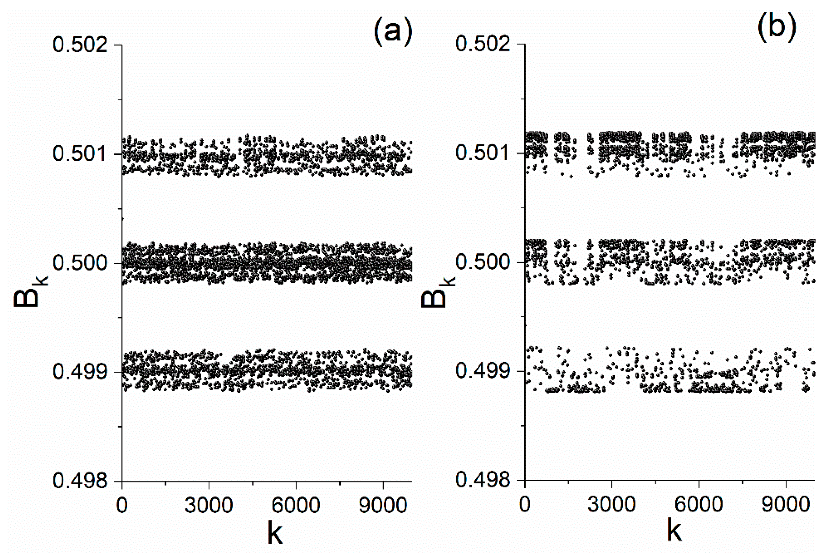
Figure 2. The transformation of a symbolic time series into a magnetic field through the device of Figure 1 using PA with $c<1$ (here $c=0.1$): (a) For currents directions determined by a random time series. (b) For currents directions determined by the 2D-Ising symbolic dynamics at spin lattice site (15,88) in critical state.

Figure 2. The transformation of a symbolic time series into a magnetic field through the device of Figure 1 using PA with $c<1$ (here $c=0.1$): (a) For currents directions determined by a random time series. (b) For currents directions determined by the 2D-Ising symbolic dynamics at spin lattice site (15,88) in critical state.

In Figure 2, we present the magnetic field produced by the device of Figure 1 according to PA, i.e., according to Equation (4), in the cases that the flow directions of the rings’ currents are determined by the symbolic time series produced by a random number generator (Figure 2a), and by the values of the spin at a randomly selected point of a ${100}^2$ lattice of 2D-Ising for temperature $T=T_c=2.308$ (Figure 2b). In both cases, the values $a=1$, $d=10$, $c=0.1$, $I=1$, and $N=10,000$ were used for the parameters of the device of Figure 1 for the calculation of the magnetic field values presented in Figure 2. In both cases, the transformations are performed from the time domain (t) to the space domain (ring positions $k$). Each spatial pattern of the magnetic field is unique, determined by the respective symbolic dynamics.

We will now investigate whether one can infer the dynamics of each symbolic time series by studying the resulting magnetic field values in the space domain, i.e., for different ring positions $k$. Specifically, we will check the distributions of the “$k$ waiting lengths”, $L$, i.e., the spatial lengths corresponding to numbers of consecutive ring positions yielding magnetic field values at a specific value level or within a specific value zone, which is the analogous of waiting times (laminar lengths) in the space domain. If the dynamics of the symbolic time series are indeed imprinted in the resulting magnetic field values in the space domain, one would expect that the distributions of the “$k$ waiting lengths” should be: exponential for the case (a) and power-laws for the case (b), respectively, according to the corresponding time domain statistics (waiting times distributions) of each driving time series. This would indicate the completeness of the transformation act performed by the device. Beyond that, the study of the resulting magnetic field distribution in the space domain could be used to characterize the dynamic state of a system that can produce symbolic time series by quantitatively evaluating the intermediate states between randomness and criticality.

As a first step, one must determine the magnetic field values or value zones for which the “$k$ waiting lengths” is reasonable to be calculated. By observing Figure 2, it is clear that for values $c<1$ (here $c=0.1$) three zones appear in the positive half-plane, and, respectively, three symmetric zones in the negative half-plane (not shown in Figure 2), within which the fluctuations of the magnetic field values are the main characteristic. It is therefore reasonable to use one of these zones, e.g., the central positive zone, for the calculation of the “$k$ waiting lengths” and the study of their distribution.

Figure 2a shows that the borders of the central positive zone are the values $0.50022$ and $0.49978$ of the magnetic field. Thus, we must calculate the values that the number, $L$, of consecutive ring positions $k$ for which the magnetic field takes any value between these values, i.e., $0.49978<B_k<0.50022$, takes. Unfortunately, it turned out that the “$k$ waiting lengths” $L$ take only three (3) values, and this means that no reliable information can be extracted from their distribution. Similar results were obtained from the magnetic field depicted in Figure 2b for the central positive zone, while the selection of any other (positive or negative) zone did not lead to better results. Moreover, the results do not improve even if one increases the statistics, i.e., by increasing the number of rings (and corresponding number of time series values), $N$. The existence of zones within which many different magnetic field values fall is the reason why very long “$k$ waiting lengths”, $L$, result, thus rendering the number of different $L$ values very small.

A solution to this problem could be the “quantization” of the magnetic field, i.e., if the magnetic field could only take a very limited number of values and not be able to fluctuate within value zones. In such a case, the “$k$ waiting lengths”, $L$, are expected to have shorter lengths and consequently take a larger number of different values that would allow us to produce adequate distributions of $L$, permitting us to extract safe conclusions. As we will show in the rest of this work, this can be done through the theory of prime numbers.

Although the results presented in Figure 2 do not allow us to extract the sought quantitative information about the dynamics of the driving time series, they do provide some qualitative information. Indeed, in Figure 2b one can see the existence of a structure in the form of intermittency at all (spatial) scales for the revealed magnetic field value zones. However, the development of the phenomenon of intermittency presupposes the existence of correlations [9]. Therefore, the existence of intermittency is an indication for the existence of underlying dynamics. On the other hand, the almost homogeneous structures in Figure 2a exclude the existence of structures at all scales. Structures similar to that of Figure 2b have been presented in [10] for the order parameter of the hybrid artificial neural network in the critical state.

3. A Prime-Numbers-Based Solution

The central forces of classical physics obey mathematical laws of the form $~\frac{1}{r^s}$, where $s=2$ for the gravitational field (law of universal gravitation), electric field (Coulomb law), elementary magnetic field ($dB)$ (Biot-Savart law). Given that in all three of these fundamental forces between bodies, the sums of the forces appear in their calculations, i.e., quantities of the form ${{\displaystyle \sum }}_i\frac{1}{r_i^s}$, their convergence must be ensured. A more general expression of the harmonic series is the Riemann zeta function, which is defined as $\zeta \left(s\right)={{\displaystyle \sum }}_{i=1}^{\infty }\frac{1}{i^s}$, with $Re\left\{s\right\}>1$ [11]. Thus, within the framework of a discretization of space with unit $l$, where $r_i~i·l \left(i=1,2,\dots \right)$, the sum of the interactions can be treated as the Riemann zeta function.

One of the most famous unsolved issues in mathematics, which dates back to 1859, is the Riemann hypothesis [11,12,13] that asks where the zeros of the Riemann zeta function, $\zeta \left(s\right)$, are located. This function is an analytic complex function. For complex numbers, $s$, with real part $Re\left\{s\right\}>1$, Riemann zeta function equals both an infinite sum over all integers, and an infinite product over the prime numbers. A natural number is called a prime number if it is $>1$ and cannot be written as the product of two smaller natural numbers. Thus, by going one step further, one can “move” from the Riemann zeta function to the prime numbers through a theorem known as the Euler product [14,15], according to which one can write:

$$\zeta \left(s\right)={{\displaystyle \sum }}_{n=1}^{\infty }\frac{1}{n^s}={{\displaystyle \prod }}_{p:prime}\frac{1}{1-p^{-s}}={{\displaystyle \prod }}_{p:prime}\frac{p^s}{p^s-1}, Re\left\{s\right\}>1.$$

(6)

For a long time, the study of prime numbers has been examined as the canonical example of pure mathematics, with no applications outside of mathematics. The concept of prime numbers is so important that it has been generalized in different ways in various branches of mathematics. Beyond pure mathematics, prime numbers are used in a series of various applications. Several public-key-cryptography algorithms, such as RSA and the Diffie-Hellman key exchange, are based on large prime numbers (2048-bit primes are common) [16]. Shor’s algorithm can make any integer factor in a polynomial number of steps on a quantum computer [17]. Prime numbers are also used in pseudorandom number generators including linear congruential generators [18]. Beyond mathematics and computing, prime numbers have potential connections to quantum mechanics [19,20,21,22]. They have also been used in evolutionary biology to explain the life cycles of cicadas [23].

In this context, in the following we present an application of prime numbers to the current carrying circular rings device of Figure 1. Thus, out of the above-mentioned three central forces, here we focus on the application of prime numbers to the calculation of the magnetic field (Biot-Savart law). The connection of the zeta function [24] with the Biot-Savart theory has already been presented in [1]. In the following, we present the connection of the Riemann zeta function with the Biot-Savart theory and, furthermore, the connection with prime numbers for the first time. Specifically, we investigate to which extent can a prime-numbers-based algorithm (PNA) (presented in Section 3.1) closely approach the results of PA (see Section 1) regarding the calculation of the magnetic field of the device of Figure 1. The rapid convergence of values as ensured by Euler’s product (Equation (6)) was our motivation to introduce the prime numbers in the stratified magnetic field of the device of Figure 1 with the expectation that values convergence would turn the stratified magnetic field zones presented in Section 2 into levels of fixed values, i.e., to the sought “quantization” of the magnetic field.

3.1. The Prime-Numbers-Based Algorithm for the Calculation of the Magnetic Field

Since our intention is to introduce the harmonic series to the magnetic field calculation (Equation (4)), to lead to the prime numbers according to Equation (6), we consider the case $c^2\ll 1$. Then, given the fact that $n,m\ge 1$ and using the condition $c^2\ll 1$, we can consider the approximations for the two sums appearing in Equation (4):

$${{\displaystyle \sum }}_{n=1}^{k-1}\frac{I_{k-n}}{{\left(n^2+c^2\right)}^{3/2}}\approx {{\displaystyle \sum }}_{n=1}^{k-1}\frac{I_{k-n}}{n^3},$$

(7)

$${{\displaystyle \sum }}_{m=1}^{N-k}\frac{I_{m+k}}{{\left[m^2+c^2\right]}^{3/2}}\approx {{\displaystyle \sum }}_{m=1}^{N-k}\frac{I_{m+k}}{m^3}.$$

(8)

In Equations (7) and (8), the directions of currents $I_{k-n}, I_{n+1+k}$ appear, which, as mentioned in Section 1 and Section 2, are described by a dichotomic variable taking the values $+1,-1$, according to the corresponding symbolic time series driving the device. This fact does not allow the calculation of the above sums since these sums are dynamically alternating sequences.

Let us assume that the hypothesis that currents’ directions are determined by a symbolic time series is suspended and all currents have the same–for example, positive–direction, i.e., $I_{k-n}=+1, I_{n+1+k}=+1$, which would lead to a constant magnetic field (the same magnetic field value at all positions $k$ of the device’s axis). In such a case, one successively gets the following.

For large $k$ values, as $k\to \infty$, the sum in Equation (7) is written:

$${{\displaystyle \sum }}_{n=1}^{\infty }\frac{1}{n^3}=\zeta \left(3\right)\approx 1.20205690\dots$$

(9)

For small $k$ values and as $N\to \infty$, the sum in Equation (8) is written:

$${{\displaystyle \sum }}_{m=1}^{\infty }\frac{1}{m^3}=\zeta \left(3\right)\approx 1.20205690\dots$$

(10)

In Equations (9) and (10), $\zeta \left(3\right)$ is the Riemann zeta function $\zeta \left(s\right)$ for $s=3$, and since the condition $Re\left\{s\right\}>1$ is valid for $s=3$, one could introduce the prime numbers using Equation (6), for $s=3$:

$$\zeta \left(3\right)={{\displaystyle \prod }}_{p:prime\in \left\{1,\infty \right\}}\frac{1}{1-p^{-3}}={{\displaystyle \prod }}_{p:prime\in \left\{1,\infty \right\}}\frac{p^3}{p^3-1}.$$

(11)

As already mentioned, the effort here is to accomplish a suitable approximation that allows to introduce the Euler product (prime numbers) to the estimation of the magnetic field of the device of Figure 1. The difficulty in the studied case is to introduce the prime numbers and also to restore the hypothesis that currents’ directions are determined by a symbolic time series by appropriately introducing the information of currents’ directions.

The proposed approximate solution is a prime-numbers-based algorithm (PNA) accomplished in three steps (the segment of the code that calculates the magnetic field through the proposed prime numbers approximation for the random case, i.e., for random alternations of the signs $+1,-1$, of the currents $I_k$, is presented in the Appendix A):

• Initially, the currents’ directions are determined by a symbolic time series, e.g., a symbolic time series produced by a random generator or by a dynamic system, such as 2D-Ising, etc. Specifically (see also Section 1), for a two-symbol time series $x\left(t_i\right)$ of length $N$ ($i=1,2,\dots , N$) a device of $N$ current carrying circular rings (Figure 1) is considered. In all rings, the current has the same intensity $I=1$, but the flow direction $I_k$ in each ring (taking values $+1,-1$) is determined by the corresponding time series symbol in such way that the symbol of $x\left(t_1\right)$ determines the current flow direction $I_1$ of the ring at the position $k=1$, the symbol of $x\left(t_2\right)$ determines the current flow direction $I_2$ of the ring at $k=2$, and so on. For example, for $i=k=1$, if $x\left(t_1\right)=-1$, then $I_1=-1$, while if $x\left(t_1\right)=+1$, then $I_1=+1$, etc.
• In a second step, the above determined directions are not yet taken into account and all currents are considered as having the same direction, $I_k=+1$. In this case, the sums appearing in Equation (4) are approximated as shown in Equations (9) and (10) (for $c^2\ll 1$) and, using Equation (11), prime numbers are introduced in their calculation, allowing the fast convergence to $\zeta \left(3\right)$ value. In the practical implementation, the $\zeta \left(3\right)$ Riemann zeta function is calculated using the first 168 prime numbers (i.e., employing all $p<1000$), since it is found that the $\zeta \left(3\right)$ value converges up to the 8th decimal. Therefore, for large $k$ values, the following first approximation is done: ${{\displaystyle \sum }}_{n=1}^{\infty }\frac{1}{n^3}={{\displaystyle \sum }}_{m=1}^{\infty }\frac{1}{m^3}=\zeta \left(3\right)\approx {{\displaystyle \prod }}_{p:prime\in \left\{1,1000\right\}}\frac{p^3}{p^3-1}$. Of course, in cases that lower or higher accuracy in the calculation of $\zeta \left(3\right)$ value is sought, one can employ less or more prime numbers, respectively, in the calculations.
• Finally, an iterative procedure is proposed, comprising of a nested loop that introduces the actual signs (directions) of $I_{k-n}, I_{k+m}$, and $I_k$ to the magnetic field values’ calculation, $B_k$, at each position $k$. Specifically, at each outer loop step, the two inner loops (Inner Loop 1 & Inner Loop 2 in the Appendix A) calculate the corresponding “sign-corrected Riemann zeta function” by introducing the signs of the currents (determined in the first step) to the Riemann zeta function value (calculated during the second step), by implementing the following products: ${{\displaystyle \prod }}_{n=1}^{k-1}{I}_{k-n}\zeta \left(3\right)$ (denoted as “piA” in the Appendix A) and ${{\displaystyle \prod }}_{m=1}^{N-k}{I}_{m+k}\zeta \left(3\right)$ (denoted as “piB” in the Appendix A). Actually, the inner loops suggest the following approximation for the Equations (7) and (8), respectively: ${{\displaystyle \sum }}_{n=1}^{k-1}\frac{I_{k-n}}{{\left(n^2+c^2\right)}^{3/2}}\approx {{\displaystyle \sum }}_{n=1}^{k-1}\frac{I_{k-n}}{n^3}~{{\displaystyle \prod }}_{n=1}^{k-1}{I}_{k-n}\zeta \left(3\right)$ and ${{\displaystyle \sum }}_{m=1}^{N-k}\frac{I_{m+k}}{{\left[m^2+c^2\right]}^{3/2}}\approx {{\displaystyle \sum }}_{m=1}^{N-k}\frac{I_{m+k}}{m^3}~{{\displaystyle \prod }}_{m=1}^{N-k}{I}_{m+k}\zeta \left(3\right)$. The outer loop calculates the magnetic field values, $B_k$, using Equation (4), the sign of each current $I_k$, and the “sign-corrected Riemann zeta function” values, calculated in the corresponding inner loops, in place of the two sums of Equation (4). Therefore, it finally calculates the following approximate value for $B_k$: $B_k~\frac{1}{2}{\alpha }^2{d}^{-3}I\left\{\frac{I_k}{c^3}+{{\displaystyle \prod }}_{n=1}^{k-1}{I}_{k-n}\zeta \left(3\right)+{{\displaystyle \prod }}_{m=1}^{N-k}{I}_{m+k}\zeta \left(3\right)\right\}$, i.e., $B_k~\frac{1}{2}{\alpha }^2{d}^{-3}I\left\{\frac{I_k}{c^3}+{{\displaystyle \prod }}_{n=1}^{k-1}\left(I_{k-n}{{\displaystyle \prod }}_{p:prime\in \left\{1,1000\right\}}\frac{p^3}{p^3-1}\right)+{{\displaystyle \prod }}_{m=1}^{N-k}\left(I_{m+k}{{\displaystyle \prod }}_{p:prime\in \left\{1,1000\right\}}\frac{p^3}{p^3-1}\right)\right\}$.

It is clear that in the above-presented proposed algorithm, there is mathematical gap concerning the way the signs of the currents are introduced in the calculation, since the hypothesis that the approximations ${{\displaystyle \sum }}_{n=1}^{k-1}\frac{I_{k-n}}{n^3}~{{\displaystyle \prod }}_{n=1}^{k-1}{I}_{k-n}\zeta \left(3\right)$ and ${{\displaystyle \sum }}_{m=1}^{N-k}\frac{I_{m+k}}{m^3}~{{\displaystyle \prod }}_{m=1}^{N-k}{I}_{m+k}\zeta \left(3\right)$ are valid cannot be rigorously proven. However, the numerical experiments presented in Section 4 prove that PNA provides a reasonable approximation of the actual magnetic field (calculated using PA), as well as the very important feature of “quantization” of the magnetic field, which is necessary in order to be possible to proceed with the analysis of “$k$ waiting lengths” distribution, as explained in Section 2. Importantly, the results obtained by the analysis of the “$k$ waiting lengths” distribution (after having applied PNA) prove that the dynamics of the analyzed symbolic time series are successfully uncovered (see Section 5). Moreover, it should be mentioned that, as proven during the applications runs, the PNA is almost 20 times faster than the PA for the same data.

4. Quantization of the Magnetic Field Using the Prime-Numbers-Based Algorithm

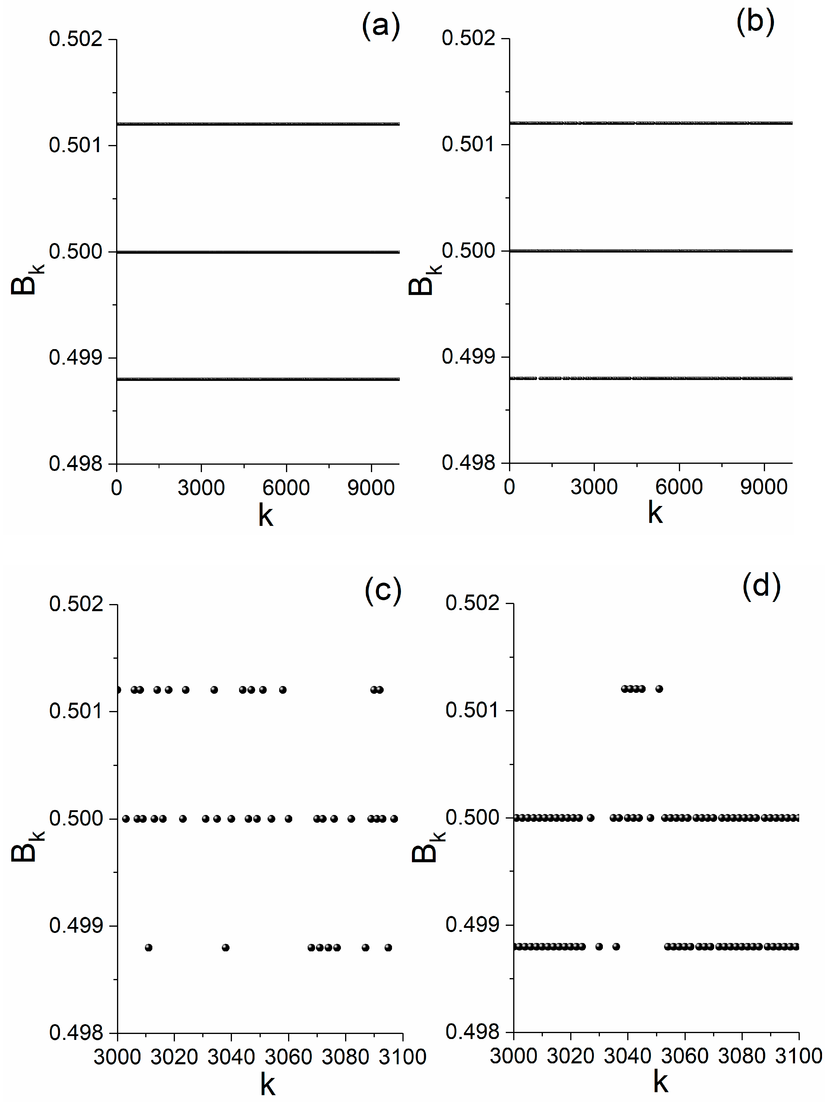
In Figure 3, we present the results obtained using the approximate algorithm PNA (see Section 3.1) for the calculation of the magnetic field of the device of Figure 1, for the same symbolic time series used in Section 2, i.e., in case (a) produced by a random number generator, and in case (b) produced by 2D-Ising in critical state. Moreover, the same parameters were used for the device as in the PA obtained results presented in Section 2, namely, $a=1$, $d=10$, $c=0.1$, $I=1$, and $N=10,000$.

From Figure 3a,b, we observe that the use of PNA led to the following interesting result: PNA eliminated the three magnetic field value zones produced by the PA (Figure 2a,b respectively), yielding in their place three distinct levels, i.e., “quantized” values, of the magnetic field. Specifically, by using PNA, three distinct levels appear in the positive half-plane and, respectively, three symmetric levels in the negative half-plane (not shown in Figure 3). Moreover, as apparent from Figure 3c,d, the magnetic field value does not remain the same for long lengths of consecutive ring positions $k$. As mentioned in Section 2, this provides a solution in the problem of extracting adequate distributions of the “$k$ waiting lengths”, $L$, since they have shorter lengths and consequently take a larger number of different values. Therefore, the “quantization” of the magnetic field by using PNA indeed provided a solution to the problem of studying the dynamics of the driving symbolic time series that emerged in the case that the magnetic field fluctuates within zones of values (see also Section 2).

Finally, it is important to note that the “quantized” magnetic field is a kind of coarse graining of the real magnetic field that seems to be more compatible to the notion of symbolic dynamics. Consequently, the specific transformation from the time domain (t) to the space domain (ring positions $k$) performed by the device of Figure 1 using the PNA, may be reasonable for one to expect that could carry over the dynamics of the driving symbolic time series to the spatial allocation of the “quantized” magnetic field. Thus, the rest of the paper focuses on the application of PNA to symbolic time series aiming at revealing their dynamics by analyzing the statistics of the spatial information of the resulting magnetic field–specifically, the distribution of the “$k$ waiting lengths”.

Although this is not so important for our approach, at this point we would like to discuss the question of whether PNA produces a reasonable approximation of the real magnetic field. The PNA could be considered to provide a reasonable approximation of the magnetic field produced by the PA if the middle values of the fluctuation zones of the PA results (Figure 2) were very close to the values of the quantized fixed levels of the PNA results (Figure 3). Indeed, by comparing Figure 2 and Figure 3, one can verify that the values of the two sides (upper and lower) of the magnetic field fluctuation zones of Figure 2 are clearly related to the two sides (upper and lower) of the quantized magnetic field values of Figure 3, $B_k=0.4987$, and $B_k=0.5012$, respectively. Specifically, $B_k=0.4987$ lower-bounds the lower fluctuation zone of Figure 2 and $B_k=0.5012$ upper-bounds the upper fluctuation zone of Figure 2. Moreover, the middle quantized magnetic field value of Figure 3 coincides with the middle of the central zone of Figure 2 ($B_k=0.500$).

It is also interesting that in the case of the random time series (case (a)) for $N=1000$ rings (the rest of the parameters were kept the same with the ones used to produce the results of Figure 2 and Figure 3), it was found that the probabilities with which the PA calculated magnetic field values that are distributed to the three fluctuation zones of Figure 2a are 24%, 45.5%, and 30.5%, for the upper, central, and lower zone, respectively. Interestingly, for the case of PNA, the corresponding probabilities are 23%, 46%, and 31%. These results are almost the same for both algorithms, confirming the fact that the PNA approximation is very close to the real results. As ones approaches the asymptotic limit (for example $N=30,000$), then both algorithms converge in the probability ratio 1:2:1 for upper, central, and lower zones, respectively.

Taking into account all the above-mentioned evidence, we deem that the PNA can be considered a reasonable approximation of PA.

5. Analysis of the Quantized Magnetic Field Produced by Symbolic Dynamics Sequences

In this Section, we analyze the spatial information of the results presented in Figure 3. Specifically, the distribution of “$k$ waiting lengths”, $L$, (see Section 2) of the quantized magnetic field values of the device of Figure 1 driven by symbolic time series, as calculated by the PNA, is calculated. The objective is to find out whether the symbolic dynamics of the currents’ directions sequence are reflected in the quantized magnetic field values, as estimated by the PNA, by quantifying how far or close the dynamics of the system are to randomness. As already mentioned in Section 2, if the dynamics of the symbolic time series are indeed imprinted in the resulting magnetic field values in the space domain, one would expect that the distributions of the “$k$ waiting lengths” should be: exponential for the case (a) and power-laws for the case (b), respectively, according to the corresponding time domain statistics (waiting times distributions) of each driving time series.

As already mentioned in Section 4, the equivalent of the central zone of Figure 2—that was selected in Section 2 for the analysis of “k waiting lengths”, in the quantized magnetic fields of Figure 3—is the positive central fixed level $B_k=0.5$ (the same for both cases (a) and (b)). Therefore, our analysis focuses on the calculation of the “k waiting lengths” at this central fixed magnetic field value. Specifically, we calculate the lengths $L$ by counting the number of consecutive ring positions for which the quantized magnetic field values is $B_k=0.5$. Namely, we sequentially scan the ring positions; the counting, for each case, starts as soon as the magnetic field takes the value $B_k=0.5$, and the counting is continued as long as the magnetic field in consecutive ring positions keeps taking this value; as soon as the magnetic field takes any other positive or negative value, the counting is interrupted, and so on.

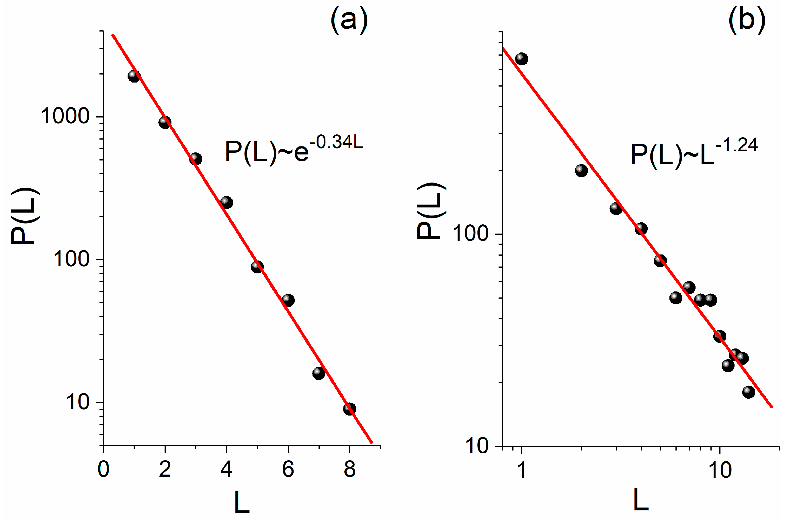
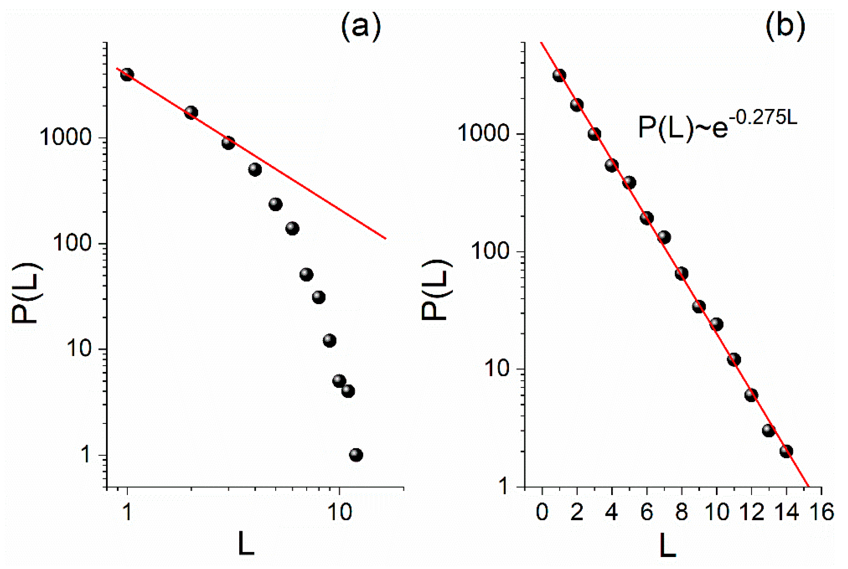
Figure 4 presents the obtained distributions of the “$k$ waiting lengths”, $L$, for the two symbolic time series, using the following parameters for the device of Figure 1: $a=1$, $d=10$, $c=0.1$, $I=1$, and $N=30,000$. Note that we chose to repeat the arithmetic experiment of Figure 3 for a higher $N$ value, which ensures the convergence of the magnetic field distributions to the different zones/quantized values (see Section 4) for PA and PNA, respectively. We should mention, however, that even if the results of Figure 3 are used, the “$k$ waiting lengths” distributions of Figure 4 practically remain unchanged.

From Figure 4a,b it can be confirmed that the symbolic dynamics of the currents’ directions sequence are indeed reflected on the magnetic field values as estimated by the PNA. Therefore, the PNA is consistent with the results expected, which means that it preserves the two following basic behaviors of dynamic systems, that is:

(a)

the exponential distribution of waiting times in “time series” that randomness dominates, and

(b)

the power-law distribution of waiting times in “time series” that are produced from critical states (critical points) of natural systems.

The information provided by the waiting times’ distribution is important for time series analysis, including the analysis of symbolic time series. The “$k$ waiting lengths”, $L$, at the quantized magnetic field value, produced by the PNA, can therefore indeed be considered a space-domain-analogue to the waiting times at specific symbols of the driving time series, as expected (see also Section 6). In direct analogy to what happens for waiting times in the time domain, in the space domain, an exponential distribution of the “$k$ waiting lengths” means that the long lengths are cut. Thus, in such cases, the long-range correlations and the dynamics produced by them are absent. The quantitative evaluation of how close the system is to randomness can be inferred by means of the value of the negative factor in the exponent of the exponential distribution (its absolute value is often called “the rate parameter”). The more negative the factor is (the higher the rate parameter), the narrower the (short) lengths range included the distribution, the closer the system is to randomness. At the opposite end of the complete absence of dynamics, the “full dynamics” case exists, characterized by the presence of all scales of lengths $L$, from the very short up to very long lengths, which could be equal to the size of the system. The distribution of these lengths is mathematically expressed by power-laws. Thus, between the two extreme behaviors–that is, the exponential and the power-law–all real systems’ dynamic behaviors can be found, while their dynamic state can be inferred by the “$k$ waiting lengths” distribution, quantitatively evaluating the intermediate states between randomness and criticality. As mentioned in Section 2, we chose to study the two extreme distributions of “$k$ waiting lengths”, i.e., the exponential and the power-law, as an indication of the completeness of the transformation act performed by the device. Therefore, the study of the quantized magnetic field can be an autonomous method that can be used to provide a quantitative indication of how close or far the dynamics of a system is from each end, i.e., randomness, on one hand, and extended dynamics at all scales as it appears at the critical point on the other hand.

In order to demonstrate the ability of the device of Figure 1–using PNA for the calculation of the quantized magnetic field–to respond to changes in the time series that determines the current directions’ sequence, we present Figure 5. Specifically, Figure 5a shows the deviation from the power-law of Figure 4b if the 2D-Ising time series is produced for a temperature higher than the pseudocritical ($T=3.2>T_c$), whereas Figure 5b shows the distribution of “$k$ waiting lengths” if one imposes in the data which gave the power-law of the Figure 4b a form of shuffling (surrogate type). In the latter case, an exponential distribution results with a rate parameter close to the exponent of the randomness case presented in Figure 4a.

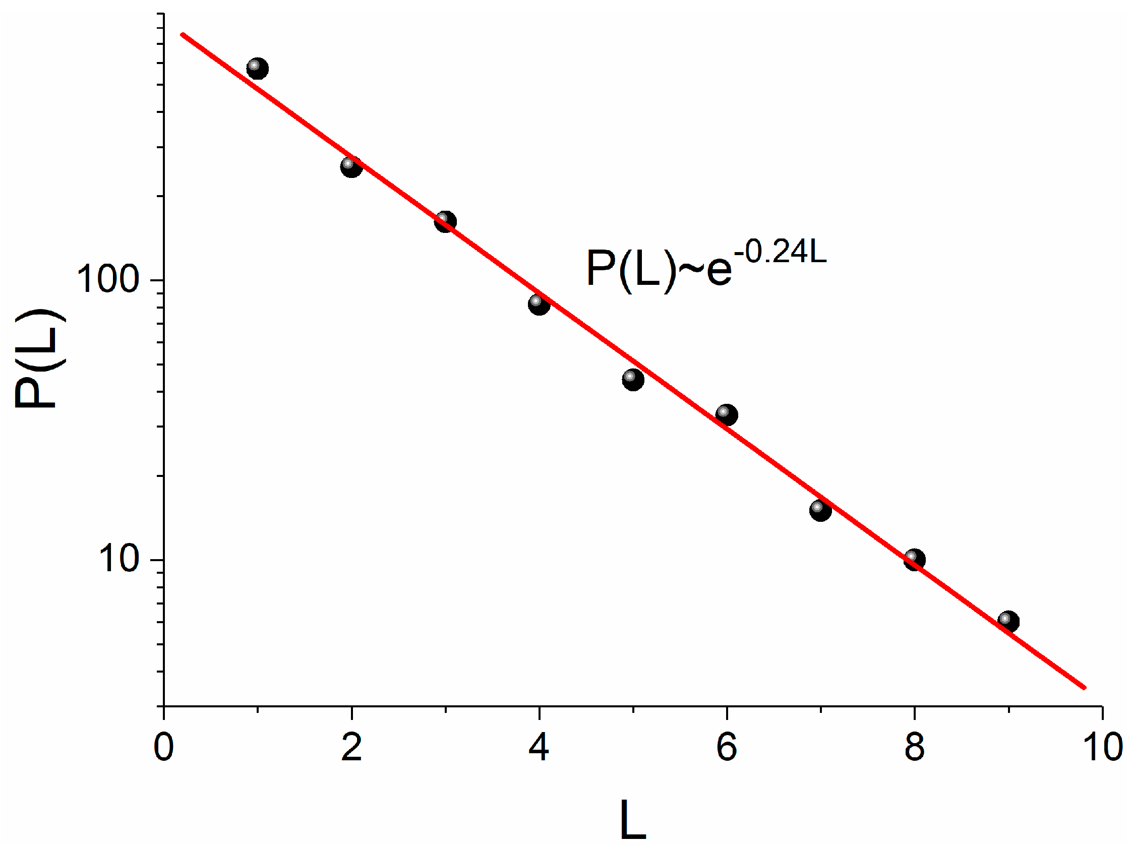
A Real Example: The DNA Sequence Case

The example presented in this section refers to a human (Homo sapiens) gene. The DNA is a sequence of four bases, Adenine, Guanine, Cytosine, and Thymine, denoted by the letters A, G, C, T, respectively. Bases A, G belong to the category of purines and bases C, T to the category of pyrimidines. Thus, we could express the DNA sequence of the GAPDH (Glyceraldehyde-3-Phosphate Dehydrogenase) gene of the Homo sapiens, as a sequence of purines and pyrimidines, that is as a symbolic “time series” of the symbols “$+1$”, “$-1$”. After turning the gene into a symbolic “time series”, it was used as the driving time series to determine the currents’ directions of the device of Figure 1, and the PNA was applied to calculate a quantized approximation of the magnetic field, as presented in Section 4, whereas the distribution of the corresponding “$k$ waiting lengths” was calculated as presented in Section 5. The results are shown in Figure 6.

As shown in Figure 6, the value of the negative factor in the exponent of the exponential distribution is higher than the corresponding exponent value of a random sequence ($-0.24>-0.34$) (Figure 4a). This means that longer lengths survive. Thus, in contrast to a random sequence, the human gene presents some kind of structure. The correlations that are responsible for this structure must have organized the coding part of the gene. Finding quantitative relationships between a large number of genes through the use of the PNA methodology is a challenging task for a future study. It will also be interesting in the future to use the Blocked Bloom Filter methodology in genome assemblies [25], where prime numbers are used in the random string algorithms.

In this example, we saw that a pure mathematical theory such as prime numbers, combined with a device of physics such as a device of current carrying circular rings, is able of extracting biological information from a biological structure such as DNA.

6. The PNA-Algorithm-Based Symbolic Time Series Analysis Compared to Time Domain (Waiting Times) Analysis

As already mentioned in Section 2, the stratified magnetic field value zones, produced for $c<1$ by the studied current carrying circular rings device, present a symmetry around zero, while the introduction of prime numbers for the approximate calculation of the magnetic field values results to three positive and their symmetrical three negative fixed magnetic field value levels (see Section 4). In the analysis results presented in Section 5, the calculation of the “$k$ waiting lengths” at the positive central magnetic field value was considered.

It might have seemed an arbitrary choice to use the positive central field value for the calculation of the “$k$ waiting lengths”. However, we will show that this is not so and that the specific choice is directly connected to the driving time series structure, i.e., to the use of two symbols. When one performs the analysis of a two-symbol time series in the time domain, then the only way is to use waiting times at one of the two symbols. For the case of the random two-symbol time series (case (a)), keeping the same $a$ and $I$ parameters of the device ($a=1$, $I=1$), at the limit $c\ll 1$, e.g., $c=0.002$, the magnetic field values produced by the device using PNA converge to two fixed magnetic field values, $B_k=\pm 0.5$. This result means that when the distance between consecutive rings is large compared to ring diameter ($c\ll 1$) the two symbols “$\pm 1$” are mapped by the device to the magnetic field values $B_k=\pm 0.5$. As the consecutive rings distance is reduced (so that $c<1$), the “quantized” magnetic field of Figure 3a (see also Figure 3c) appears, where, as already pointed out, two phenomena are observed. First, three distinct levels appear in the positive half-plane and, respectively, three symmetric levels in the negative half-plane, where in each half-plane the central level is $B_k=+0.5$ and $B_k=-0.5$, respectively. Second, as shown in Figure 3c, the existence of a structure in the form of intermittency at all (spatial) scales around the central level. Therefore, each central level value can be considered to correspond to one of the symbols of the driving symbolic time series, so it is reasonable to study the “$k$ waiting lengths” at one of the central values–e.g., the positive one.

It is also interesting to investigate what happens for the two extreme time series cases considered in Section 5, if one applies the analysis (i) to the “$k$ waiting lengths” at the negative central magnetic field value (the symmetrical to the positive central one), and (ii) directly to the driving time series in the time domain, i.e., by analyzing the waiting times at each of the symbols (“$-1$” and “$+1$”). For the ease of the reader, the results obtained for the abovementioned cases are summarized in

Table 1. Analysis of “$k$ waiting lengths” and waiting times distributions for the symbolic time series produced by (a) a random number generator and (b) the 2D-Ising symbolic dynamics at spin lattice site (15,88) in critical state.

	“k Waiting Lengths” Distribution		Waiting Times Distribution
	At the Positive Central Value	At the Negative Central Value	$\mathbf{At} “+1” \mathbf{Symbol}$	$\mathbf{At} “-1” \mathbf{Symbol}$
Random	$P\left(L\right)~e^{-0.34L}$ (Figure 4a)	$P\left(L\right)~e^{-0.33L}$	$P\left(L\right)~e^{-0.32L}$	$P\left(L\right)~e^{-0.31L}$
2D-Ising	$P\left(L\right)~L^{-1.24}$ (Figure 4b)	$P\left(L\right)~L^{-1.56}$	$P\left(L\right)~L^{-1.24}$	$P\left(L\right)~L^{-1.59}$

along with the corresponding results presented in Figure 4. It is mentioned that out of the total values of the driving symbolic time series ($N=\mathrm{30,000}$), the random case, as expected, presented an almost symmetrical distribution of the two symbols ($N_{“-1”}=15,029$, $N_{“+1”}=14,971$), while in the 2D-Ising case the “$+1$” symbol appeared more frequently than the “$-1$” symbol ($N_{“-1”}=12791$, $N_{“+1”}=17,209$).

Table 1 Analysis of “$k$ waiting lengths” and waiting times distributions for the symbolic time series produced by (a) a random number generator and (b) the 2D-Ising symbolic dynamics at spin lattice site (15,88) in critical state.

Table 1 shows that the analysis of the “$k$ waiting lengths” at the negative central magnetic field value yields almost the same results as the analysis of the “$k$ waiting lengths” at the positive one for the random case, where the distribution of the two symbols is almost symmetrical but leads to different results (higher exponent) for the 2D-Ising case. Moreover, the time-domain analysis (using the waiting times of the driving time series) showed that for the random case, almost the same exponents as the ones of the “$k$ waiting lengths” analysis were found for both symbols. On the other hand, for the 2D-Ising time series, the analysis resulted in different exponents for the waiting times at the “$+1$” symbol and for the waiting times at the “$-1$” symbol, whereas the exponent calculated for the waiting times at “$+1$” was the same as that obtained for the “$k$ waiting lengths” at the positive central value.

At this point, it must be clarified that in the case of 2D-Ising, if one increases the statistics, i.e., if a long enough time series is produced by prolonging simulation runs, the power-law exponents obtained for the waiting times at each symbol will eventually be the same. For example, after increasing the length to $N=150,000$, the probabilities of appearance of the two symbols become very close (49–51%) and the power-law exponents for the “$-1$” symbol and the “$+1$” symbol were found to be $1.40$ and $1.37$, respectively—i.e., much closer than the ones presented in Table 1 (for $N=30,000$). By further increasing $N$, these two exponents will converge to the same value. However, this cannot be done for real systems’ time series, especially if these are of relatively short length.

As already mentioned, the only way to analyze a two-symbol time series in the time domain by means of waiting times is to use waiting times at one of the two symbols. In case one of the symbols appears more often than the other, which is the usual case for (finite-, much more for short-, length) time series resulting from real dynamical systems, then the result depends on the symbol at which the waiting times are calculated for. Therefore, in such a case, although the existence of dynamics can be revealed by the scaling behavior of waiting times, the quantitative result is ambiguous; the involved exponent cannot be definitely determined, since the exponent’s value depends on the considered symbol.

On the other hand, when one performs the analysis in the space domain, using the “$k$ waiting lengths”, the problem is mitigated in the following way. There are six possible magnetic field values (three positive and their symmetrical three negative). Instead of analyzing “$k$ waiting lengths” at the positive or the negative central magnetic field value, one can calculate the “$k$ waiting lengths” at both of them, considering the rest four possible values as values “interrupting $k$ waiting”. That is, as long as the magnetic field values at consecutive ring positions, $k$, keep taking any the two central field values, the magnetic field is considered to be waiting at these values and the “$k$ waiting length” is increasing; as soon as the magnetic field takes any other positive or negative value, the “$k$ waiting” is interrupted. Consequently, a single distribution of “$k$ waiting lengths” is obtained, which has taken into account the dynamics of both symbols of the original symbolic time series. Therefore, the exponents resulting from the above-described approach could be considered as a quantitative expression of the dynamics of the original system, without the inherent ambiguity of the time domain analysis as of which symbol best describes the system’s dynamics. It is worth investigating in the future how close this estimate is to the actual exponents by analyzing systems whose exponents are known. However, Section 7 presents an example corroborating the view that the specific approach is indeed able to expose the real dynamics of a complex system that can be described in terms of two-symbol symbolic dynamics.

7. An Example Demonstrating the Usefulness of the Proposed Symbolic Time Series Analysis Method

In this section, we present an application of the proposed PNA-algorithm-based, symbolic time series analysis method to an artificial neural network (ANN). Through the specific application, the usefulness of the analysis method is demonstrated for systems that can be studied in terms of two-symbol symbolic dynamics.

As already mentioned in previous sections, the dynamics of a system can be revealed through the study of the distribution of waiting times (directly in the time domain). For a two-symbol symbolic dynamics time series, the information of this distribution can be extracted very simply, as long as the probabilities of appearance of the two symbols are exactly equal, i.e., 50%-50%. As already demonstrated in Section 6, any deviation from this rule leads to waiting times distributions that are different for the two symbols, and, consequently, the values of the exponents calculated for the corresponding waiting times distributions are different. Therefore, the quantitative result is ambiguous; the involved exponent reflecting the dynamics of the system cannot definitely be determined since the exponent’s value depends on the considered symbol. Especially for real systems’ time series of relatively short length, for which the statistics cannot be changed (as in the case of simulation results where one can increase the statistics by just prolonging simulation time), the problem is evident. As it is shown in the following, the application of the proposed PNA-algorithm-based symbolic time series analysis by taking into account the dynamics of both symbols of the original symbolic time series, as suggested in Section 6, that is by calculating the “$k$ waiting lengths” at both the positive and the negative central magnetic field values, provides a unique way to expose the real dynamics of such a complex system.

7.1. The Hybrid Spin Model

In the following, we briefly present the key concepts of a hybrid spin model (HSM) that has recently been proposed [10] by combining concepts of ANNs with the stochastic dynamics of Ising spin lattices. The reader is referred to [10] for details on the HSM.

We focus on quantized states in an ANN by considering a network of $n$ neurons, whose output states are random variables ${\xi }_i\left(t\right), i=1,2,\dots ,n$ that can take the values $+1$ or $-1$. Each neuron of the network connects to all others comprising an extensive feedback structure spanning over the whole network. Moreover, the connection weights $w_{ij}$ may take either positive or negative values, reflecting synaptic properties in the connection between two neurons. Then, according to the ANN formalism, the energy function representing the state of the HSM at time $t$ is given by:

$$E\left(t\right)=-{{\displaystyle \sum }}_{i,j=1}^n{w}_{ij}{\xi }_i\left(t\right){\xi }_j\left(t\right)$$

(12)

The quantity $1/\beta$ is considered the control parameter of the HSM. As it is known [10,26], such a quantity corresponds to the temperature of a thermal system that undergoes a phase transition of second order. Then, a local field could be $m_i\left(t\right)$, which under the consideration ${\beta }_i=\beta$ takes the same value for all neurons [10]:

$$m_i\left(t\right)=\tan \mathrm{h}\left(\frac{\beta }{2}E\left(t\right)\right),$$

(13)

where $t$ is the algorithmic time of the model [10].

The mean field of all neurons is estimated as [10]:

$$Field\left(t\right)=\frac{{{\displaystyle \sum }}_{i=1}^n{m}_i\left(t\right)}{n}.$$

(14)

The HSM presents similarities with spin systems at thermal equilibrium, such as Ising models, defined on lattices of various forms and dimensions–usually two or three dimensions. An effective algorithm that produces configurations at thermal equilibrium is the Metropolis algorithm, whose basic principle is the second law of Thermodynamics which describes the energy minimization in macroscopic systems. According to this algorithm, the configurations at constant temperature are selected with Boltzmann statistical weights, i.e., $e^{-\beta H}$, with $H$ the Hamiltonian of the spin system. In the case of nearest neighbor interactions, $H$ is given by Equation (5). The main differences of the HSM from the Ising models are: (a) in the HSM no lattice structures are considered and thus the interactions between the neurons extend over the entire network, and (b) in the HSM the Boltzmann statistics have been replaced with the Fermi statistics that considers spins as fermions [10].

7.2. Analysis of the HSM Time Series

Let us consider an HSM of $n=20$ neurons, with a control parameter $1/\beta =2.3$. For the specific HSM, the time series of the quantity $Field\left(t\right)$ was produced according to Equation (14), for the algorithmic time $t=1,2,\dots ,150,000$. For the Metropolis algorithm that produces the $Field\left(t\right)$ time series, $J_{ij}=1$ has been considered in the calculation of $H$ (see Equation (5)). The choice of the above-mentioned value for the control parameter in an HSM with $n=20$ has been thoroughly justified in [10]. 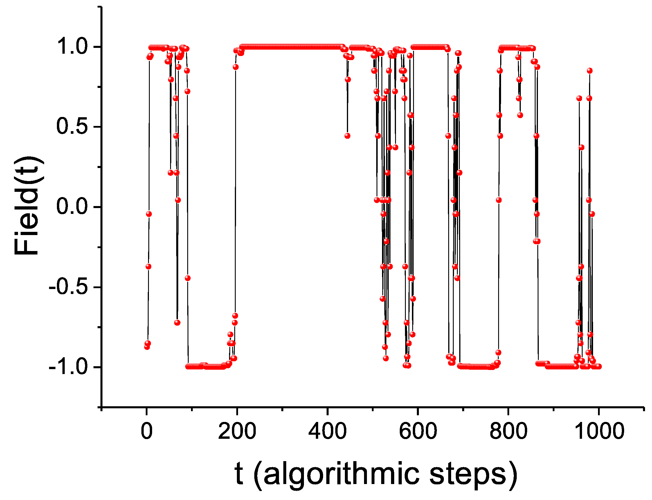Here it is just mentioned that for $1/\beta =2.3$, and under the appropriate initial conditions, it has been found that the lengths of the waiting times extend to all scales, which leads to the conclusion that for the specific value of the control parameter, the HSM is in its critical state [10].

Figure 7 presents a 1000-points-long segment of the produced $Field\left(t\right)$ time series to show the typical variation of $Field$ vs. the algorithmic time $t$.

In order to proceed with the analysis, the whole obtained HSM $Field\left(t\right)$ time series ($150,000$ values) is first converted into a two-symbol symbolic dynamics time series by corresponding positive values to the “$+1$” symbol and negative values to the “$-1$” symbol. In the resultant symbolic dynamics time series, the probability of appearance of each symbol, “$-1$” and “$+1$”, was 47.5% and 52.5%, respectively.

If one performs an analysis of waiting times (i.e., directly in the time domain), as already mentioned, one can take into account only one of the symbols. Consequently, there are two options to determine the distribution of the waiting times, $L_t$, from which the dynamics of the HSM is expected to be revealed: (a) by considering as waiting times the number of consecutive time points that the time series remains at the symbol “$+1$”, which are interrupted by the waiting times at the symbol “$-1$”; and (b) by considering the waiting times at the symbol “$-1$”. 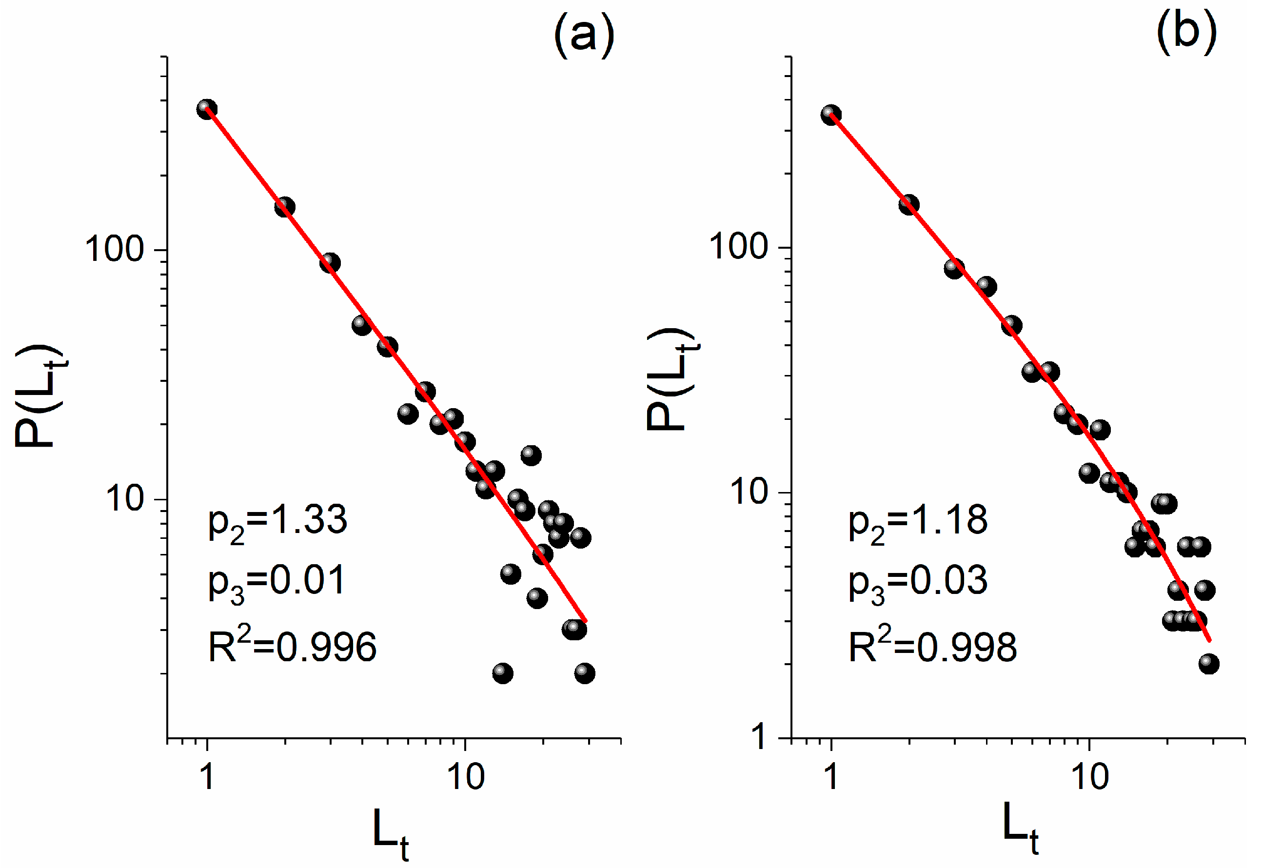As it has been shown in Section 6, if the probabilities of appearance of the two symbols are the same, then the exponents of the distributions obtained by these two ways would be the same. Here, however, there is a deviation from this symmetry. In Figure 8, the results for these two waiting times distributions are presented.

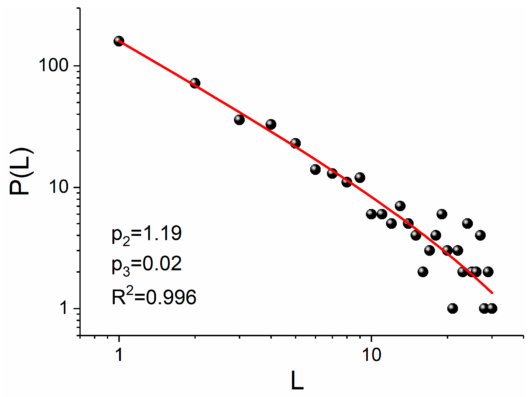
The fitting line has been derived using the fitting function $f\left(x\right)=p_1{x}^{-p_2}{\mathrm{e}}^{-p_{3}x}$ that is usually employed to calculate the critical exponents [8]. The fitting result for the distribution of Figure 8a (since $p_2=1.33$ and $p_3\approx 0$) is the power-law $P\left(L_t\right)~L_t{}^{-1.33}$, whereas for the distribution of Figure 8b (since $p_2=1.18$ and $p_3\approx 0$) is the power-law $P\left(L_t\right)~L_t{}^{-1.18}$. The observed asymmetry in the symbolic dynamics, i.e., in the probability of occurrence of “$+1$” (52.5%) and “$-1$” (47.5%), is the reason that the exponents obtained for the two considered waiting times analysis options are different.

The first observation is that both distributions of Figure 8 are very close to the power-law. As it has been mentioned in the previous sections, this indicates critical state; that is, the considered HSM is in critical state. The second observation is that the exponents $p_2$ that quantitatively reflect these critical dynamics are quite different, although the probabilities of occurrence of the two symbols do not significantly differ. To understand how important this difference is, the concept of universality classes from the theory of critical phenomena is used. As it has been shown in [8], the exponent of the power-law, $q$ (i.e., $p_2$ of the $f\left(x\right)$ fitting function), above the critical point is directly connected to one of the 6 critical exponents, specifically to the exponent $\delta$ (isothermal exponent) with the relation:

$$q=1+\left(1/\delta \right).$$

(15)

Using Equation (15) and the above-presented results, it is found that for case of the “$+1$” branch of the time series, the exponent $\delta$ is calculated to be $\delta =3$, which indicates the MFT (mean field theory) universality class, whereas for the case of the “$-1$” branch the calculated exponent $\delta$ is very close to $\delta =5$, which indicates the 3D-Ising universality class [5]. Thus, beyond the information about the existence of criticality, the particular dynamic evolution inferred by the value of the exponent $q$ is completely different if calculated for each branch separately.

From the above-presented results, it is clear that the waiting times analysis (analysis of the symbolic time series in the time domain) leads to an ambiguity about the dynamics of the examined HSM; no specific conclusion can be drawn. As mentioned in Section 6, the only way to mitigate this problem is to apply the proposed PNA-algorithm-based symbolic time series analysis by taking into account the dynamics of both symbols of the original symbolic time series, i.e., by calculating the “$k$ waiting lengths” at both the positive and the negative central magnetic field values ($+0.5$, $-0.5$), considering the rest four possible values of the magnetic field as values “interrupting $k$ waiting”.

In the Figure 9, we present the results obtained from the PNA-algorithm-based symbolic time series analysis by taking into account the dynamics of both symbols.

Using once again the fitting function $f\left(x\right)=p_1{x}^{-p_2}{e}^{-p_{3}x}$ on the distribution of the “$k$ waiting lengths” of Figure 9, since $p_2=1.19$ and $p_3\approx 0$, the result is $P\left(L\right)~L^{-1.19}$. The power-law exponent $q\left(=p_2\right)=1.19$ indicates the 3D-Ising universality class. This result is consistent with that of the dynamics of the HSM described by the Metropolis algorithm, and thus it follows the dynamic evolution of the Ising models. Therefore, the proposed PNA-algorithm-based symbolic time series analysis carried out by taking into account the dynamics of both symbols of the original symbolic time series proved to be able to uncover the specific dynamics of the HSM, allowing us to recognize how such an ANN evolves dynamically over time. Another important outcome is that this result also confirms that the HSM is a complex system because the exponent $q$ does not come out as an average value of the corresponding exponents obtained for each one of the two branches (“$-1$” and “$+1$”) of the time series if taken separately, nor is it affected by the statistics of the two symbols.

The application presented for the HSM is considered an important application as with the specific ANN it has recently been possible to achieve a simulation of the real biological neuron, where the neuron spikes but also the dynamics of the fluctuations in the inter-spike time interval were successfully reproduced [27]. Two very interesting applications of the proposed PNA-algorithm-based symbolic time series analysis to real systems are currently in the process of implementation. Specifically, related to the dynamic behavior of strong earthquake preparation processes [28] and memristors [29].

8. Conclusions

Any symbolic time series of two symbols, that can emerge from a dynamical system, can be transformed through the device of Figure 1 into a magnetic field, whose values are stratified. Through the application of an algorithm based on the theory of prime numbers–the PNA–it is possible to convert this field into a field of quantized values. This allows the reproduction of the waiting times’ distribution of the symbolic dynamics time series in the space domain (ring positions $k$), in the form of the distribution of the “$k$ waiting lengths”, $L$, from which the dynamics of the system can be determined. Therefore, the spatial allocation of the values of such a magnetic field can be considered as a “fingerprint” of the dynamics of the system that produces the symbolic time series. We confirmed this result with two extreme examples of dynamics, referring to (a) the random generation of the “$+1$”, “$-1$” symbols through a random number generator, and (b) the sequence of $+1$, $-1$ spin states of a lattice point of the 2D-Ising model in critical state. Moreover, the symbolic sequence produced by the DNA of the GAPDH (Glyceraldehyde-3-Phosphate Dehydrogenase) human gene was also successfully analyzed as a real-world, intermediate dynamics case.

In the case that the analyzed two-symbol time series is of relatively short length and one of the symbols appears more often than the other–which is the usual case for time series resulting from real dynamical systems–the analysis in the time domain, i.e., by means of waiting times, can only be applied to one of the symbols, leading to ambiguous quantitative result; the involved exponent cannot be definitely determined, since the exponent’s value depends on the considered symbol. On the contrary, the proposed space domain analysis can be applied by taking into account the dynamics of both symbols, i.e., a single distribution of “$k$ waiting lengths” is obtained, which has taken into account the dynamics of both symbols of the original symbolic time series. Thus, the resulting exponents could be considered as a quantitative expression of the dynamics of the original system, without the inherent ambiguity of the time domain analysis as of which symbol best describes the system’s dynamics. This unique feature of the proposed analysis method was confirmed by successfully inferring the universality class of an artificial-neural-network-based hybrid spin model by the value of the critical exponent $\delta$, whereas for the same example, the analysis of waiting times led to an ambiguous quantitative result.

We consider that the suggested approach offers a new perspective in the study of complex systems that could offer a unified way of studying diverse complex systems, which is something that remains to be explored in depth in the future. For example, one could apply the suggested analysis to other artificial neural networks, where two-symbol symbolic time series can be produced by corresponding the symbols to inhibitory/excitatory states, to magnetic or photonic materials, or polarization systems, corresponding the two symbols to polarization states, logic circuits, two-state switches, stock-market time series, after an appropriate symbolic coarse-graining, symbolic representations of sociological, humanistic or linguistic data, etc.

However, beyond the applications, the introduction of the theory of prime numbers in the study of natural phenomena is in itself an important fact that has conceptual extensions.