Optimal Design of Convolutional Neural Network Architectures Using Teaching–Learning-Based Optimization for Image Classification

Abstract

Convolutional neural networks (CNNs) have exhibited significant performance gains over conventional machine learning techniques in solving various real-life problems in computational intelligence fields, such as image classification. However, most existing CNN architectures were handcrafted from scratch and required significant amounts of problem domain knowledge from designers. A novel deep learning method abbreviated as TLBOCNN is proposed in this paper by leveraging the excellent global search ability of teaching–learning-based optimization (TLBO) to obtain an optimal design of network architecture for a CNN based on the given dataset with symmetrical distribution of each class of data samples. A variable-length encoding scheme is first introduced in TLBOCNN to represent each learner as a potential CNN architecture with different layer parameters. During the teacher phase, a new mainstream architecture computation scheme is designed to compute the mean parameter values of CNN architectures by considering the information encoded into the existing population members with variable lengths. The new mechanisms of determining the differences between two learners with variable lengths and updating their positions are also devised in both the teacher and learner phases to obtain new learners. Extensive simulation studies report that the proposed TLBOCNN achieves symmetrical performance in classifying the majority of MNIST-variant datasets, displays the highest accuracy, and produces CNN models with the lowest complexity levels compared to other state-of-the-art methods due to its promising search ability.

1. Introduction

Various machine learning and deep learning models, such as feedforward neural networks (FNNs) [1], convolutional neural networks (CNNs) [2,3], and recurrent neural networks (RNNs) [4,5], were introduced in order to tackle different real-world tasks, such as object recognition [6,7,8], speech emotion recognition [9], fault detection [10,11,12,13,14,15], classification [16,17,18], and estimation problems [19]. In recent years, deep learning models, such as CNNs, have gained overwhelmed popularity due to their superiority over human experts in tackling certain tasks [20]. CNNs consist of two major components, known as feature extractor and classifier, that enable them to complete assigned tasks effectively without requiring manual pre-processing of raw data. With proper training of a CNN network, the convolution and pooling layers incorporated into feature extractor can automatically extract meaningful features from the raw input data and then feed into the fully connected layers of the classifier to perform the designated tasks with promising performance.

Optimal design of network architecture is one of the fundamental cornerstones that govern the network performance of CNN. Despite having promising performances, the network architectures of most existing CNN models, such as GoogleNet [21], AlexNet [22], InceptionNet [21], VGG [23], DenseNet [24] and ResNet [25], are handcrafted by designers with extensive knowledge of problem domains [26]. These manual processes of designing CNN architecture are not only time consuming but also computationally expensive due to their trial-and-error natures. These manually designed network architectures might also have limited flexibility in handling different datasets with unique data distributions and hence, their performance may be compromised. Ideally, the optimal design of CNN network architectures should be automatically guided by the characteristics of given problems without requiring significant intervention from human experts to provide insights about specific problem domains. It is also notable that the majority of the manually handcrafted CNN models consist of redundant trainable parameters that lead to complex, network-heavy computational efforts. Hence, an efficient algorithm with symmetrical performance in achieving good classification accuracy and constructing CNN architectures with low complexity levels is worthy of investigation.

To alleviate the drawbacks of trial-and-error design, different strategies were devised to systematically determine the optimal network architectures of a CNN. These network architecture design methods are divided into three categories: (a) reinforcement-learning-based methods [27], (b) gradient-based methods [28], and (c) metaheuristic-search-based methods [29]. Baker et al. [30] proposed a reinforcement-learning-based method known as MetaQNN that utilized ten graphical processing units (GPUs) running on a CIFAR-10 dataset for ten days. For the reinforcement-learning-based method proposed by Zoph and Le [31], 800 GPUs were used to train the optimal CNN network architecture with CIFAR-10 for 28 days. Although reinforcement-learning-based methods can deliver promising performances, they are not feasible for researchers with limited computational resources. Gradient-based methods, such as those proposed by Liu, Simonyan, and Yang [28] are more efficient than reinforcement-learning-based methods, but the former methods did not have strong theoretical supports, and the CNN network architectures obtained were unstable. The construction of optimal CNN network architectures using gradient-based methods was also computationally expensive and required significant involvement from experts with rich domain knowledge. Finally, metaheuristic-search-based methods can design the optimal CNN network architectures by employing metaheuristic search algorithms (MSAs) without requiring any insights about specific problem domains. MSAs are population-based algorithms in which the search operators inspired by different natural phenomena are used to locate the global optimum iteratively and are used to solve optimization problems. Some notable MSAs include the genetic algorithm (GA) [32], particle swarm optimization (PSO) [33], differential evolution (DE) [34], and teaching learning-based optimization (TLBO) [35]. Given their appealing features, such as simple implementation, gradient-free characteristics, and strong global search ability, these MSAs are widely utilized to solve different real-world optimization problems [36,37,38,39,40,41,42,43,44,45,46].

Although the benefits of MSAs enable them to be naturally employed to optimize CNN network architectures, this optimization remains as a challenging task because of some newly arisen issues. For instance, the optimal CNN network architecture required to solve a particular dataset is unknown prior to the task. It is crucial to design a proper solution-encoding strategy that can facilitate the searching of CNNs with different network architectures (i.e., in terms of depths, layer types, etc.) when handling different problems. Appropriate constraints must also be defined to avoid the construction of invalid CNN network architectures in solution spaces without compromising the ability of MSAs to find novel architectures. Existing MSAs are originally designed to solve global optimization problems with specified dimensional size in a continuous search space. The optimization of CNN network architecture is more challenging than typical global optimization because it involves searching for solutions with different dimensional sizes (i.e., CNNs with different depths and combinations of layers) within the same solution space. Referring to the adopted solution encoding strategy, appropriate modifications must be made to the original search operators of MSAs to accommodate the searching of CNNs with flexible types of network architectures in solution space. When using population-based MSAs to optimize CNN network architectures, another concern is the time and computational resources required to evaluate the fitness value of each candidate solution. A computationally efficient fitness evaluation process is needed to ensure the practicability of MSAs in designing optimal CNN network architectures. Finally, it is notable that only classical MSAs (e.g., GA, PSO, and DE) are employed in optimizing the network architectures of CNNs despite the emergence of new MSAs inspired by different natural phenomena due to the “No Free Lunch Theorem” [47]. While these new MSAs can deliver promising optimization performances when solving standard benchmark functions, it is essential to further investigate their potentials and feasibilities for handling increasingly challenging real-world problems, such as the optimization of CNN network architectures.

This paper aims to propose an effective and efficient network architecture design method to achieve symmetrical tradeoff between classification accuracy and network complexity. In particular, a relatively new MSA known as TLBO is employed to automatically search for the optimal network architecture of a CNN based on a given dataset without requiring human intervention. An appropriate solution-encoding strategy and design constraints are first defined for TLBOCNN, enabling it to search for the valid CNN network architectures with flexible sizes in the solution space. To ensure the practicability of TLBOCNN, a computationally efficient fitness evaluation process is employed to measure performance differences between the CNN network architectures represented by different TLBOCNN learners. Appropriate modifications are also proposed for the search operators of TLBOCNN during the teacher and learner phases, enabling the computation of population mean and new solutions from existing TLBOCNN learners with different lengths.

The remaining sections of this paper are organized as follows. Related works and research contributions of the current work are presented in Section 2. The overall search mechanisms of the proposed TLBOCNN are described in Section 3. Extensive simulation studies conducted for the performance evaluation of the proposed TLBOCNN are reported in Section 4. Finally, the conclusion and future works are summarized in Section 5.

2. Related Works

2.1. Teaching–Learning-Based Optimization (TLBO)

TLBO is inspired by the teaching and learning processes of an actual classroom [35]. At the initialization stage, all learners are randomly generated with a population size of N in the search space. Each nth learner is considered as a candidate solution for solving the given problem and defined as $X_n=\left[X_{n,1},\dots ,X_{n,d},\dots ,X_{n,D}\right]$, where $n\in \left[1,N\right]$ refers to the population index $d\in \left[1,D\right]$ and D refer to the dimension index and the total dimensional size of the problem, respectively. Meanwhile, the quality or fitness level of each nth learner is denoted as $f\left(X_n\right)$.

During the teaching phase, the new solution of each nth learner can be obtained by learning from the difference between the best learner (i.e., teacher) and the population mean (i.e., mainstream knowledge of classroom), represented as $X^{teacher}$ and $X^{mean}$, respectively. The mainstream knowledge of classroom $X^{mean}$ is first expressed as:

$$X^{mean}=\frac{1}{N}{\displaystyle \sum }_{n=1}^N{X}_n$$

(1)

Given $X^{mean}$, the new solution of each nth learner, denoted as $X_n^{new}$, is calculated as:

$$X_n^{new}=X_n+r_1\left(X^{teacher}-T_f{X}^{mean}\right)$$

(2)

where $r_1\in \left[0,1\right]$ is a random number generated from uniform distribution; $T_f\in \left\{1,2\right\}$ is a teaching factor that determines the importance of $X^{mean}$ in updating each learner.

For the learner phase of TLBO, a peer interaction mechanism is simulated to update each nth learner. Define $p\in \left[1,N\right]$ as the index of a randomly selected peer learner to be compared with each nth learner, where $p\ne n$. Let $f\left(X_n\right)$ and $f\left(X_p\right)$ be the fitness values of learners $X_n$ and $X_p$, respectively. For minimization problems, the new solution of nth learner $X_n^{new}$ can be obtained from the learner phase as:

$$X_n^{new}=\{\begin{array}{cc}{X}_n+r_2\left(X_p-X_n\right),\hfill & \hfill \mathrm{if}f\left(X_p\right)<f\left(X_z\right)\\ X_n+r_2\left(X_n-X_p\right),\hfill & \hfill \mathrm{otherwise}\end{array}$$

(3)

where $r_2\in \left[0,1\right]$ is a random number generated from uniform distribution. At the end of both the teacher and learner phases, the fitness value of $X_n^{new}$ for each nth learner is evaluated as $f\left(X_n^{new}\right)$ and compared to $f\left(X\right)$. If $f\left(X_n^{new}\right)$ is better than $f\left(X_n\right)$, the current $X_n$ is replaced by new $X_n^{new}$. Otherwise, $X_n^{new}$ is discarded. The knowledge enhancement of each TLBO learner through both teacher and learner phases is repeated until the termination criteria are satisfied. The teacher solution $X^{teacher}$ is then obtained as the best solution found for a given problem.

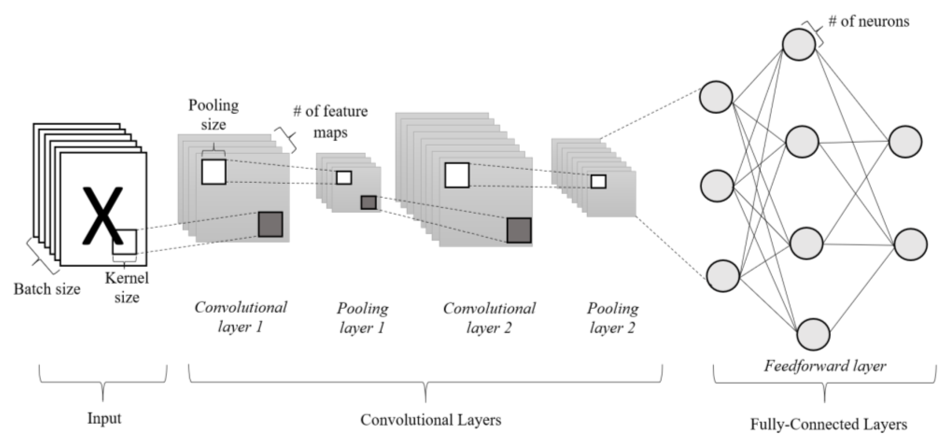
2.2. Convolutional Neural Networks (CNNs)

CNNs [48] are introduced as the combination of a feature-learning module with a trainable classifier, where the latter consists of at least one fully connected layer. Feature-learning modules aim to replace manual feature-extracting processes used in conventional machine learning methods to minimize the error due to data pre-processing. Contrary to FNNs, CNNs are applied directly to the raw data. After learning meaningful features from raw data, these features are then fed into the subsequent layer of trainable classifiers. The architecture of a sequential CNN is illustrated in Figure 1, where the feature learning module consists of two convolutional layers and two pooling layers, whereas the trainable classifier has three fully connected layers.

For each convolution layer, the filters with predefined filter width and filter height are first initialized. Then, the convolutional process is applied to the input images to generate feature maps. Each filter is first slid from the leftmost to the rightmost side of the input image with a step size defined as stride width. The filter is then moved downward with a step size known as stride height and slid through the input image from left to right again. This sliding process is repeated until the filter reaches the bottom-right of the input images and produces a complete feature map in which each feature map element is obtained as the sum of products for elements of filter and the corresponding elements of input images that overlap with filter. The number of filters required to produce a feature map is equal to number of channels defined in the input images. The connection weights in the filter are the learnable parameters in the convolution layer, whereas the hyperparameters considered during convolutional process include the width and height of filters, the number of filters, the number of feature maps, the width and height of stride, and the type of convolution.

The pooling layer is used for downsampling the feature maps produced by convolution process to achieve local translation invariance. During the pooling process, a kernel is first initialized with the predefined kernel width, kernel height, and types of pooling. Two popular operations used in the pooling layers are maximum pooling and average pooling. For maximum pooling, the maximum values of elements in patches of feature maps overlapped with the kernels are identified. Meanwhile, the average pooling is used to calculate the average values of elements observed in the patches of feature maps that overlap the kernel. The sliding process of the kernel is performed from the top-left to the bottom-right of input images based on the predefined stride width and stride height to obtain the downsampled feature maps. Contrary to the convolution layer, the pooling layer does not contain any learnable parameters. The hyperparameters involved in the pooling process include the kernel width and kernel height, the stride width and stride height, and the pooling type (i.e., maximum or average pooling).

The training of the CNN aims to minimize the errors between the predicted outputs of the network and the actual outputs stored in datasets. The trainable parameters of the CNN are optimized with gradient descent and backpropagation by minimizing cross-entropy loss. A simple CNN, such as that illustrated in Figure 1, may consist of a few hundred thousand to millions of trainable parameters. Depending on the network architectures of the CNN, the training process could consume up to several weeks even with the use of high-performance graphical processing units (GPUs). Given the time-consuming process of evaluating multiple CNNs, it is not feasible to design the network architecture of CNN using a trial-and-error approach. It is crucial to develop efficient network architecture design methods that can automatically determine the optimal CNN network architectures based on given datasets without requiring rich expert domain knowledge.

2.3. Existing Metaheuristic-Search-Based Methods in Optimizing Neural Networks

Given the gradient-free characteristics, MSAs are envisioned as competitive solutions for solving challenging black-box optimization problems, such as the optimal design of neural network architectures. The idea of neuroevolution was incepted two decades ago when MSAs were used to evolve the weights or architectures of small- or medium-sized artificial neural networks (ANNs). Due to the drawbacks of the backpropagation method, such as its high tendency of becoming trapped in local optima, MSA was initially used to update the weights of ANN with fixed network architectures [49]. Despite having greater exploration strength to address local optima issues, MSAs require longer durations to train the weights of ANN than backpropagation does [50]. Sophisticated neuroevolution algorithms known as topology- and weight-evolving artificial neural networks (TWEANNs) were introduced to optimize the weights and architectures of ANNs simultaneously. Some popular TWEANNs include the Neuroevolution of Augmenting Topologies (NEAT) [51], Evolutionary Acquisition of Neural Topologies (EANT) [52], and Hypercube-Based Neuroevolution of Augmenting Topologies (HyperNEAT) [53]. A natural evolution concept of GA was adopted by NEAT [51] to evolve ANNs from simpler to more complicated architectures by increasing connection weights. Speciation was also incorporated to preserve the population diversity of NEAT while searching for more complex networks. It is infeasible to represent complex network architectures with high dimensional sizes using the direct encoding scheme of NEAT due to the excessive computational efforts required. EANT [52], with inner and outer layers, was also designed to evolve ANNs from simpler to more complex structures. The inner layer was used to govern the exploitation behavior of EANT by using evolution strategy to determine the optimal weight parameters of the network. The outer layer of EANT was more explorative because a mutation strategy was incorporated to evolve the network architectures. HyperNeat [53] used an indirect encoding strategy known as a connective compositional pattern producing network (CPNN) to represent the complex network architectures more efficiently by considering the given problem geometry. HyperNeat has worse performance than humans in solving classification problems, and it was recommended as a feature extractor for other machine learning algorithms instead [54].

There are growing trends of applying MSAs to optimize the network architectures of complex deep neural networks (e.g., CNN). PSO [33], inspired by the swarm behavior of animals in food searching, is a popular MSA used to find the optimal network architectures of CNNs. A PSO-based CNN (CNNPSO) was proposed in [3] to optimize the weights of a CNN for solving handwriting recognition problems with better accuracy. Although CNNPSO was able to solve the MNIST dataset [55] with a classification accuracy of 95% within four epochs, the processing time incurred was longer than that of a conventional CNN. A hybrid of PSO and stochastic gradient descent (PSO-SGD) was proposed in [56] to optimize the weights of a CNN by leveraging the explorative and exploitative behaviors of PSO and SGD, respectively. The connectivity weights of CNN were initialized using PSO, and then, a weight-training process was performed by SDG for a small number of iterations. The performance of PSO-SGD was evaluated using image datasets known as MNIST [55], CIFAR-10 [57], and SVHN [58]. Despite outperforming most contemporary approaches in terms of classification accuracy, the computational efforts required by PSO-SGD to solve these datasets remain unknown, and the network architecture of PSO-SGD was not optimized. In [59], an indirect encoding strategy inspired by internet protocol (IP) was used by IPPSO to represent each particle as a potential network architecture. Each IPPSO particle can search for the optimal CNN network architecture within the predefined boundary limits while preserving its population diversity. The CNN architectures obtained by IPPSO have limited preset maximum lengths and are only used to solve three-image datasets. The IP-based encoding strategy of IPPSO also required frequent conversion of parameters between binary and decimal values. Thus, the particles encoded as CNNs with deeper architectures tend to require longer computational time. In [60], psoCNN was designed to automatically search for deep neural network architectures to solve given classification problems. A direct encoding strategy and novel velocity update operator were designed for psoCNN to search for the optimal CNN architectures with rapid convergence speed. Similarly, a PSO-based architecture optimization (PSOAO) algorithm was proposed in [61] to evolve the flexible convolutional auto-encoder (FCAE). An x-reference method was used by PSOAO to determine the differences of particles with variable lengths before updating the velocity and position of particles.

Genetic algorithm (GA) [32] and genetic programming (GP) [62] are two popular MSAs inspired by Darwin’s theory of evolution and are widely used for CNN optimization. A CNN was proposed in [63] to solve the detection problems. To address the premature convergence issues of the backpropagation method, the potential weights of CNNs were encoded into the chromosomes and a standard GA was then used to train these connection weights. Despite producing a 92% success rate, the results obtained by this approach did not significantly outperform the backpropagation method. In [64], a human action recognition technique using GA and CNN was proposed. The initial weights of the CNN classifier were optimized with GA by minimizing classification error. A gradient descent algorithm was applied to further train the CNN classifier during the fitness evaluation of GA. Despite having a good accuracy of 99.98% when classifying UCF50 dataset [65], this approach only focused on the weight-updating process without optimizing the network architecture of the CNN. A multi-node evolutionary neural network for deep learning (MENNDL) was proposed in [66] by using GA to optimize the hyperparameters of CNN. MENNDL can identify the visited regions of hyperparameter space based on the results obtained from previous generation when solving the CIFAR-10 dataset [57]. A neural architecture design method known as evolving deep convolutional neural network (EvoCNN) was proposed in [67] to solve image classification problems. A variable-length gene encoding strategy was adopted by EvoCNN to represent CNNs with different depths. The connection weights of EvoCNN were also encoded with a novel representation scheme to prevent premature convergence. A self-adaptive mutation neural architecture search algorithm (SaMuNet) was designed in [68] to automatically design the optimal CNN architecture for a given problem without requiring expert knowledge. Three types of mutation strategies (i.e., adding, removing, and replacing) were introduced and selected adaptively by SaMuNet to evolve CNN architectures with better exploration strengths. A selection scheme based on semi-complete binary competition was introduced for SaMuNet to preserve the elite solutions during optimization. A GP approach was proposed in [69] to automatically construct CNN architectures and solve image classification problems with better accuracy. A direct encoding scheme inspired by the Cartesian genetic program (CGP) [70,71,72] was employed to represent the network structure and connectivity weights of CNN with better flexibility. Although the GP approach has better performance than its compared methods in solving CIFAR-10 datasets [57], excessive computational efforts were required.

Differential evolution (DE) is another popular MSA used to optimize the weights or architectures of deep neural networks. A DE-based CNN (DECNN) for searching for optimal CNN architectures with a refined version of the IP encoding strategy for was proposed in [73]. The refined IP encoding strategy of DECNN has eliminated the constraint of maximum network depth by representing a layer and its corresponding parameter with a single 2-byte IP address. Meanwhile, the overall information of CNN model was stored in the position vector of DE constructed by multiple two-byte IP address. Although DECNN can produce significantly better classification accuracy than IPPSO when solving six MNIS-variants datasets, both methods incurred high computational times due to the indirect encoding strategy used for network architecture representation. Another DE-based CNN (DE-CNN) was proposed in [74] for performing sentiment analysis in Arabic. Each parameter to be optimized (i.e., filter sizes, number of neurons, number of filters per convolutional filter sizes, initialization mode, and dropout rate) was stored in every dimensional component of the individual DE-CNN solution. Although DE-CNN has better performance than its peers in terms of classification accuracy and computational time, it has limited flexibility in terms of the construction of network architectures. An improved DE-based CNN (IDECNN) was proposed in [75] by incorporating a variable-length direct encoding strategy to represent network information with better flexibility. Each solution of IDECNN was stored with its unique parameters that represented the length of network, parameters of each layer, and sequence of layers. A new refined strategy was also used by IDECNN to effectively compute the differences between two encoded network structures during optimization. IDECNN exhibited better performance than 20 peer algorithms in terms of classification accuracy when solving eight image datasets.

2.4. Technical Contributions of Current Works

The research contributions of this paper can be summarized as follows:

• A new network architecture design method known as TLBOCNN is proposed to automatically discover the optimal network architecture of CNNs (i.e., number of layers, type of layers, kernel sizes, number of filters, and number of neurons) for image classification without requiring rich expert domain knowledge. To the best of the authors’ knowledge, no existing studies or only limited works have employed TLBO for the optimization of CNN network architectures.
• TLBOCNN can accommodate the searching of CNN network architectures with flexible size by incorporating the appropriate solution-encoding strategy and design constraints for TLBO learners with variable lengths. These modifications not only prevent the construction of CNNs with invalid network architectures but also preserve the ability of TLBOCNN in discovering novel network architectures. A computationally efficient fitness evaluation process is also incorporated into TLBOCNN to ensure the practicability of the proposed network architecture design method.
• A new mainstream architecture computation scheme is introduced in the teacher phase of TLBOCNN to determine the population mean by referring to all TLBO learners encoded as CNNs with different network architectures. In order to maintain the simplicity of TLBO, a new difference operator is first introduced in both the teacher phase and the learner phase to compare the differences between existing learners with unique network architectures, followed by the design of a new position update operator used to search for the new TLBO learners.
• Extensive simulation studies are conducted to evaluate the feasibility of proposed TLBOCNN in discovering the optimal network architectures of CNN automatically for nine popular datasets. The optimal CNN network architectures constructed by TLBOCNN are proven to have better classification performances than state-of-the-art works when solving majority datasets.

3. Details of Proposed TLBOCNN

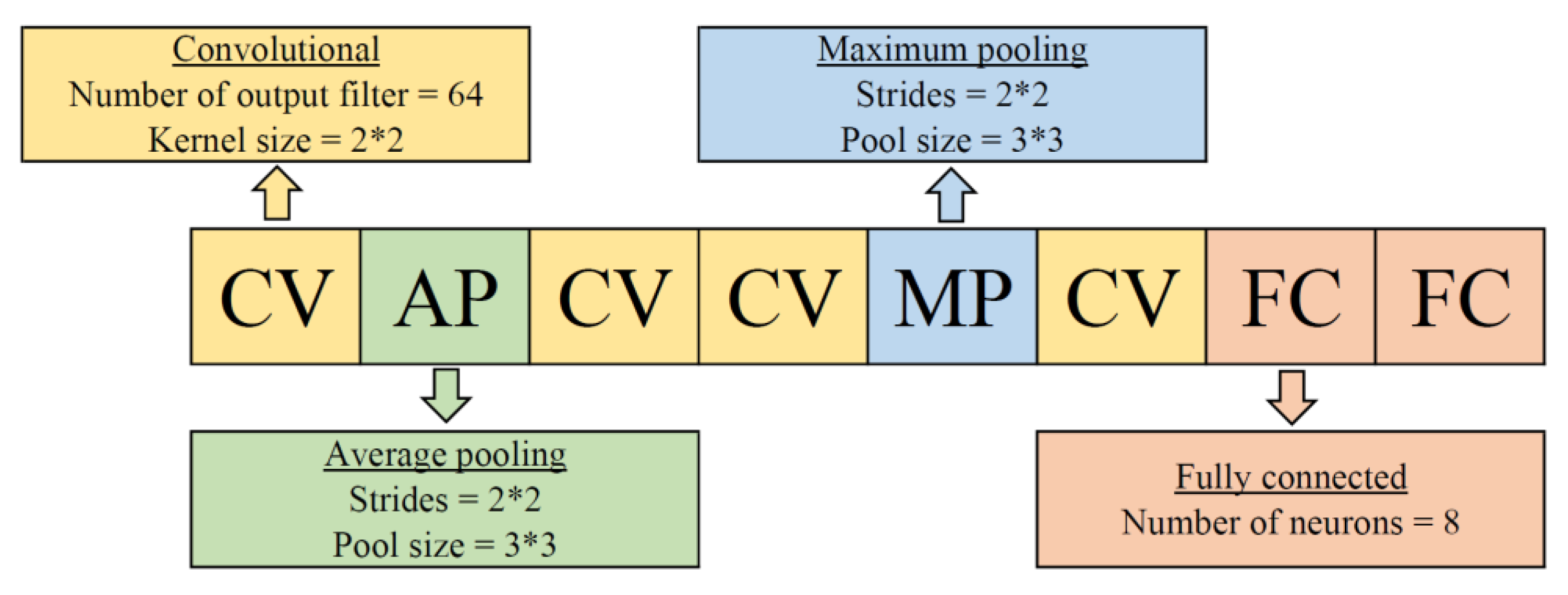
3.1. Functional Blocks Encoding Scheme

Generally, the optimal network architecture of CNN (in terms of network depth, layer types, kernel size, number of filters, number of neuron, etc.) required to solve a particular dataset is unknown beforehand because search for the best CNN network architecture should be guided based on the problem characteristics. The incorporation of an effective and efficient solution encoding scheme into TLBOCNN is therefore crucial to enable each learner to have better flexibility in searching for novel network architectures of CNNs that can solve different types of problems with desired performances.

A variable-length direct-solution encoding scheme known as the function blocks encoding scheme is incorporated into the proposed TLBOCNN. The position vector of the TLBOCNN learner is defined as a variable-length array to represent the potential CNN with unique network architecture, where each of its dimensional component is encoded as a CNN functional block along with its hyperparameters. Referring to Figure 1, three typical CNN functional blocks known as convolutional layer, pooling layer, and fully connected layer are considered when TLBOCNN is employed to automatically search for the optimal network architecture of the CNN. A functional block with the layer type of convolutional layer consists of hyperparameters, such as number of output filters and kernel sizes. For both average and maximum pooling layers, the hyperparameters are strides and pooling size. The number of neurons is included into the functional block assigned as a fully connected layer. Figure 2 shows a CNN network architecture represented by a TLBOCNN learner encoded with a list of functional blocks that consists of three convolutional layers, two pooling layers, and two fully connected layers. During the fitness evaluation process, the details of the functional block contained in each dimension of the TLBOCNN learner are decoded and compiled into the corresponding CNN network architecture for training and testing.

Depending on the types of functional block stored in each dimensional component of TLBOCNN learners, the feasible search ranges of their hyperparameters are defined to facilitate the search process of TLBOCNN within solution space. For convolutional (CV) layer, the number of output filters ($numF$) and kernel sizes ($KS$) are bounded in the search ranges of $\left[num{F}^{mi{n}^{max}}\right]$ and $\left[K{S}^{mi{n}^{max}}\right]$, respectively. For both maximum pooling (MP) and average pooling (AP) layers, the pooling size (i.e., kernel width $\times$ kernel height) and stride size (i.e., stride width $\times$ stride height) are fixed at $3\times 3$ and $2\times 2$, respectively. For the fully connected (FC) layer, the number of hidden neurons ($numNeu$) is defined in the search range of $\left[numNe{u}^{min},numNe{u}^{max}\right]$. Furthermore, the number of functional blocks ($numB$) assigned to each TLBOCNN learner can vary between $\left[num{B}^{min},num{B}^{max}\right]$ to facilitate the searching for CNNs with different network architectures (i.e., in terms of depths, types of layers, etc.) when handling different problems. The feasible search ranges of all parameters and hyperparameters considered by TLBOCNN for searching for the optimal network architecture of a CNN are summarized in

Table 1. Feasible search ranges of parameters and hyperparameters.

Type of Functional Block	Hyperparameters	Values
TLBOCNN learner	$\mathrm{Minimum}\mathrm{number}\mathrm{of}\mathrm{functional}\mathrm{blocks},num{B}^{min}$	3
	$\mathrm{Maximum}\mathrm{number}\mathrm{of}\mathrm{blocks},num{B}^{max}$	20
Convolutional (CV)	$\mathrm{Minimum}\mathrm{number}\mathrm{of}\mathrm{filters},num{F}^{min}$	3
	$\mathrm{Maximum}\mathrm{number}\mathrm{of}\mathrm{filters},num{F}^{max}$	256
	$\mathrm{Minimum}\mathrm{kernel}\mathrm{size},K{S}^{min}$	$3\times 3$
	$\mathrm{Maximum}\mathrm{kernel}\mathrm{size},K{S}^{max}$	$7\times 7$
Maximum Pooling (MP)	Pool size (i.e., kernel width $\times$ kernel height)	$3\times 3$
	Stride size (i.e., stride width $\times$ stride height)	$2\times 2$
Average Pooling (AP)	Pool size (i.e., kernel width $\times$ kernel height)	$3\times 3$
	Stride size (i.e., stride width $\times$ stride height)	$2\times 2$
Fully Connected (FC)	$\mathrm{Minimum}\mathrm{number}\mathrm{of}\mathrm{neurons},numNe{u}^{min}$	1
	$\mathrm{Maximum}\mathrm{number}\mathrm{of}\mathrm{neurons},numNe{u}^{max}$	300

.

Apart from the boundary constraints in Table 1, appropriate design constraints are also introduced for TLBOCNN to prevent the construction of invalid CNN network architectures without compromising its ability to discover the novel network architectures for different datasets. These design constraints include: (a) The first functional block assigned to each learner must be a convolutional layer; (b) the last functional block must be a fully connected layer, and the number of output neurons must equal to the number of output classes; (c) the maximum number of pooling layers assigned to each learner is restricted by sizes of input dataset. For instance, a maximum of three pooling layers is permissible for a CNN network architecture to handle input datasets with sizes of 28 $\times$ 28; (d) a fully connected layer cannot be inserted between the feature extraction modules (i.e., convolutional and pooling layers) because it can cause an overfitting issue due to the tremendous increase in trainable parameters in the CNN network architecture. If a fully connected layer is generated between the convolutional or pooling layers, all functional blocks after the fully connected layer are converted into fully connected blocks with different numbers of hidden neurons.

3.2. Population Initialization of TLBOCNN

An initial population with N learners that represents different CNN architectures (in terms of network depth, layer types, kernel size, number of filters, number of neurons, etc.) are randomly generated at beginning stage of TLBOCNN based on the function block encoding scheme, boundary constraints, and design constraints. Define $num{B}_n$ as the network depth of CNN corresponding to each nth learner that can be randomly generated between $\left[num{B}^{min},num{B}^{max}\right]$ during the initialization process. A list variable denoted as $blocks\_list$ with the size of $num{B}_n$ is also initialized as an empty list to record the type of functional block assigned to each jth dimension of the TLBOCNN learner, where $j\in \left[1,num{B}_n\right]$. The first dimension (j = 1) and last dimension (j = $num{B}_n$) of $blocks\_list$ are assigned with the convolutional and fully connected blocks, respectively, to ensure a valid CNN architecture is generated. Assume that $m_n$ is the dimension index of $blocks\_list$ when a fully connected layer is first assigned, where $m_n\in \left[2,num{B}^{max}\right]$. Once a fully connected block is recorded in the j-th dimension of $blocks\_list$ where j = m_n, the subsequent dimensions of $blocks\_list$ with the indices of $j\in \left[m_n+1,num{B}_n-1\right]$ are also assigned as fully connected blocks to satisfy the design constraints.

The remaining dimensions of $blocks\_list$ with the indices of $j\in \left[2,m_n-1\right]$ can be randomly assigned with a convolutional block or pooling block. Let $block\_type\in \left[0,1\right]$ be a value that is randomly generated with uniform distribution. If $block\_type\le 0.5$, a convolutional block is assigned to the jth dimension of $blocks\_list$. Otherwise, a pooling block is assigned when $block\_type>0.5$. Notably, a rectified linear unit (ReLU) is used as the activation function for all selected layers. Depending on the types of functional blocks selected for each jth dimension of $blocks\_list$, their corresponding hyperparameters are also randomly generated during the initialization process. For a convolutional block, the number of filters ($numF$) is randomly generated between $num{F}^{min}$ and $num{F}^{max}$, whereas its kernel size ($KS$) is randomly selected in the range of $3\times 3$ to $7\times 7$. For any jth dimension of $blocks\_list$ assigned as a pooling block, a parameter of $pooling\_type\in \left[0,1\right]$ is randomly generated with uniform distribution to select the pooling type. An average pooling block is chosen if $pooling\_type\le 0.5$, whereas a maximum pooling block is considered when $pooling\_type>0.5$. For fully connected blocks assigned in the $blocks\_list$ with indices of $j\in \left[m_n,num{B}_n-1\right]$, their numbers of hidden neurons are randomly generated as $numNeu\in \left[numNe{u}^{min},numNe{u}^{max}\right]$. Finally, the number of output neurons for the fully connected block assigned in the last dimension of $blocks\_list$ is set equal to the numbers of output classes of the dataset, denoted as numOut.

Algorithm 1 presents the population initialization process of TLBOCNN. For each nth TLBOCNN learner, the functional block information of $blocks\_list$ will be stored in the position vector of $X_n.Blocks$ after completing the initialization process. The fitness of each nth TLBOCNN learner (i.e., $X_n.Blocks$) is measured as classification accuracy, denoted as $X_n.Acc$ based on the fitness evaluation process that will be thoroughly explained later. The teacher solution of TLBOCNN, i.e., $X^{teacher}$, is obtained by identifying the initial population member with the best fitness value (i.e., highest classification accuracy).

Algorithm 1: Population Initialization
Input:N$,num{B}^{min}$,$num{B}^{max}$,$num{F}^{min}$,$num{F}^{max}$,$KS$,$numNe{u}^{min}$$,numNe{u}^{max}$, numOut
01:	Initialize $X^{teacher}.Blocks=\varnothing$ and $X^{teacher}.Acc=-Inf$;
02:	forn = 1 to N do
03:		$\mathrm{Randomly}\mathrm{generate}num{B}_n\in \left[num{B}^{min},num{B}^{max}\right]$ and $m_n\in \left[2,num{B}^{max}-1\right]$ for n-th learner;
04:		Reset the $blocks\_list=\varnothing$;
05:		forj$=1\mathrm{to}num{B}_n$do
06:			ifj = 1 then
07:				Assign $blocks\_list\left[j\right]$ with a $\mathrm{convolutional}\mathrm{block}\left(\mathrm{CV}\right).\mathrm{Randomly}\mathrm{initialize}numF$$\mathrm{between}num{F}^{min}$$\mathrm{and}num{F}^{max}$$,\mathrm{as}\mathrm{well}\mathrm{as}KS$ between $3\times 3$ $\mathrm{to}7\times 7$;
08:			else if$j=num{B}_n$then
09:				Assign $blocks\_list\left[j\right]$ with a $\mathrm{fully}-\mathrm{connected}\mathrm{block}\left(\mathrm{FC}\right)\mathrm{and}\mathrm{set}numNeu$ as numOut;
10:			else if$m\le j\le num{B}_n-1$then
11:				Assign $blocks\_list\left[j\right]$ with a $\mathrm{fully}-\mathrm{connected}\mathrm{block}\left(\mathrm{FC}\right)\mathrm{and}\mathrm{randomly}\mathrm{initialize}numNeu$ between $numNe{u}^{min}$ and $numNe{u}^{max}$;
12:			else
13:				Randomly generate $block\_type\in \left[0,1\right]$;
14:				if$block\_type\le 0.5$then
15:					Assign $blocks\_list\left[j\right]$ with a $\mathrm{convolutional}\mathrm{block}\left(\mathrm{CV}\right).\mathrm{Randomly}\mathrm{initialize}numF$$\mathrm{between}num{F}^{min}$$\mathrm{and}num{F}^{max}$$,\mathrm{as}\mathrm{well}\mathrm{as}KS$ between $3\times 3$ $\mathrm{to}7\times 7$;
16:				else if$block\_type>0.5$then
17:					Randomly generate the $pooling\_type\in \left[0,1\right]$;
18:					if$pooling\_type\le 0.5$then
19:						Assign $blocks\_list\left[j\right]$ with an $\mathrm{average}\mathrm{pooling}\mathrm{block}\left(\mathrm{AP}\right),\mathrm{where}\mathrm{the}\mathrm{pool}\mathrm{size}\mathrm{and}\mathrm{stride}\mathrm{size}\mathrm{are}\mathrm{set}\mathrm{as}3\times 3$ and $2\times 2$, respectively;
20:					else
21:						Assign $blocks\_list\left[j\right]$ with a $\mathrm{maximum}\mathrm{pooling}\mathrm{block}\left(\mathrm{MP}\right),\mathrm{where}\mathrm{the}\mathrm{pool}\mathrm{size}\mathrm{and}\mathrm{stride}\mathrm{size}\mathrm{are}\mathrm{set}\mathrm{as}3\times 3$ and $2\times 2$, respectively.
22:					end if
23:				end if
24:			end if
25:		end for
26:		$X_n.Blocks\leftarrow blocks\_list$;
27:		$\mathrm{Perform}\mathrm{fitness}\mathrm{evaluation}\mathrm{on}{X}_n.Blocks$$\mathrm{to}\mathrm{obtain}{X}_n.Acc$ with Algorithm 2;
28:		if$X_n.Acc$ $\mathrm{is}\mathrm{better}\mathrm{than}{X}^{teacher}.Acc$then     /*Compare the accuracy of n-th learner and teacher */
29:			$X^{teacher}.Blocks\leftarrow X_n.Blocks$, $X^{teacher}.Acc\leftarrow X_n.Acc$;   /*Update teacher */
30:		end if
31:	end for
Output:$P=\left\{X_1,\dots ,X_n,\dots ,X_N\right\}$

3.3. Fitness Evaluation of TLBOCNN

Fitness evaluation is essential for MSAs to measure the quality of a candidate solution when solving an optimization problem. For the proposed TLBOCNN that aims to search for an optimal design of CNN architecture, the fitness value of each learner is measured as the accuracy level of its corresponding CNN architecture when classifying the given image datasets. The learners that can produce CNN architectures with higher classification accuracies are more superior, and it will replace those with lower classification accuracies. Algorithm 2 presents the pseudocodes used to perform fitness evaluation on the new learners generated via the initialization, teacher phase, and learner phase of TLBOCNN. The fitness evaluation of each nth TLBOCNN learner is divided into two major steps: (a) training of the CNN model using training datasets and (b) evaluation of the trained CNN model using validation datasets. Detailed mechanisms of these two major steps are explained herein.

Define $Dat{a}_{train}$ as a training dataset used to train the CNN model represented by each TLBOCNN learner; it has a size of $\left|Dat{a}_{train}\right|$. The training process of CNN is performed in multiple steps, $Ste{p}_{train}$, by dividing $\left|Dat{a}_{train}\right|$ by a batch size number of $batch\_size$ as follow:

$$Ste{p}_{train}=\frac{\left|Dat{a}_{train}\right|}{batch\_size}$$

(4)

Algorithm 2: Fitness Evaluation
Input:$X_n.Blocks$, $Dat{a}_{train}$$,Dat{a}_{valid}$$,batch\_size$$,e_{train}$, ℓ
01:	Compile $X_n.Blocks$ to a full-fledged CNN;
02:	Calculate $Ste{p}_{train}$ and $Ste{p}_{valid}$ using Equations (4) and (6), respectively;
03:	$\mathrm{Initialize}\mathrm{weights}\Theta =\left\{{\theta }_1,{\theta }_2,\dots \right\}$ of complied CNN model with He Normal initializer;
04:	for$e=1$ $\mathrm{to}{e}_{train}$$\mathbf{do}$                            /* Train the compiled CNN model for$e_{train}$epoch*/
05:		for$k=1$$\mathrm{to}Ste{p}_{train}$do
06:			$\mathrm{Compute}\mathrm{the}f\left(\theta ,Dat{a}_{train,k}\right)$$\mathrm{of}\mathrm{CNN}\mathrm{model}\mathrm{based}\mathrm{on}\mathrm{its}\mathrm{current}\Theta$$\mathrm{and}Dat{a}_{train,k}$;
07:			Update the new weights ${\Theta }^{new}$ based on using Equation (5);
08:		end for
09:	end for
10:	Initialize $acc\_list\leftarrow \varnothing$ with the size of $Ste{p}_{valid}$;
11:	for$k=1$$\mathrm{to}Ste{p}_{valid}$do              /* Evaluate the compiled CNN model using validation dataset */
12:		$\mathrm{Perform}\mathrm{classification}\mathrm{on}Dat{a}_{valid,k}$$\mathrm{with}\mathrm{the}\mathrm{compiled}\mathrm{CNN}\mathrm{model}\mathrm{represented}\mathrm{by}{X}_n.Blocks$;
13:		Store the classification accuracy of complied CNN model on the $Dat{a}_{valid,k}$ into $acc\_list\left[k\right]$;
14:	end for
15:	Calculate $X_n.Acc$ of $\mathrm{compiled}\mathrm{CNN}\mathrm{model}\mathrm{represented}\mathrm{by}{X}_n.Blocks$ using Equation (7);
Output:$X_n.Acc$

To measure the fitness of each nth TLBOCNN learner, the functional block information stored in position vector $X_n.Blocks$ is decoded and compiled into a full-fledged CNN model. The trainable weights contained in all convolutional layers and fully connected layers of this CNN model are initialized using the He Normal weight initializer [20] and stored into a set variable of $\Theta =\left\{{\theta }_1,{\theta }_2,\dots \right\}$. The CNN model represented by each nth learner is trained using the Adam optimizer [76] in a predefined epoch, $e_{train}$, based on $Ste{p}_{train}$ batches of data from $Dat{a}_{train}$. In each kth training step of the CNN model where $k=1,\dots ,Ste{p}_{train}$, the corresponding cross-entropy loss is calculated as $f\left(\Theta ,Dat{a}_{train,k}\right)$ based on the current weight $\Theta$ and kth batch data $Dat{a}_{train,k}$. The new weights are updated as ${\Theta }^{new}$ by deducting the current weights stored in $\Theta$ from the product of learning rate $\ell$ and gradient of cross-entropy loss ${\nabla }_{\Theta }f\left(\Theta ,Dat{a}_{train,k}\right)$, i.e.,

$${\Theta }^{new}\leftarrow \Theta -\ell {\nabla }_{\Theta }f\left(\Theta ,Dat{a}_{train,k}\right)$$

(5)

After completing the training process, the fitness value of the trained CNN model represented by the nth learner is measured by computing its classification accuracy (i.e., $X_n.Acc$) when handling the validation dataset denoted as $Dat{a}_{valid}$ with a size of $\left|Dat{a}_{valid}\right|$. Similarly, the evaluation of trained CNN model is performed with multiple steps, $Ste{p}_{valid}$, by dividing $\left|Dat{a}_{valid}\right|$ with $batch\_size$, where

$$Ste{p}_{valid}=\frac{\left|Dat{a}_{valid}\right|}{batch\_size}$$

(6)

In each kth evaluation step of trained CNN model, its classification accuracy is calculated based on the trained weights and kth batch data of $Dat{a}_{valid}$ before storing this value into the list variable denoted as $acc\_list$. Notably, the value of classification accuracy obtained by the trained CNN model in every kth evaluation step is different due to the employment of different batch data. After all $Ste{p}_{valid}$ batch data stored in $Dat{a}_{valid}$ are evaluated, the mean classification accuracy of the trained CNN model is computed from $acc\_list$ as $X_n.Acc$ to indicate the fitness value of the nth learner, i.e.,

$$X_n.Acc=\frac{{{\displaystyle \sum }}_{k=1}^{Ste{p}_{valid}}acc\_list\left[k\right]}{Ste{p}_{valid}}$$

(7)

Evidently, the fitness evaluation process is considered the main bottleneck of the proposed TLBOCNN because each learner represents a potential CNN model with unique architecture that must be trained based on its current weights with $Dat{a}_{train}$ before its final classification accuracy can be obtained from $Dat{a}_{valid}$. It is not computationally feasible to perform full training on every potential CNN model with large training epoch numbers, $e_{train}$, especially when it involves the population-based MSAs that require searching for the optimal architecture design of a CNN in multiple iterations. This undesirable drawback can be addressed by training each potential CNN model with a smaller $e_{train}$ during fitness evaluation. Although the final classification accuracy of a potential CNN model cannot be measured accurately with a smaller $e_{train}$, the performance trends of all TLBOCNN learners during fitness evaluation can be observed, and this becomes the main consideration in assessing the quality of each learner. The potential CNN model represented by a TLBOCNN learner is more likely to have good final classification accuracy if it can perform better in several training epochs first. Full training with a higher $e_{train}$ is only performed to measure the final classification accuracy when the optimal design of CNN architecture is obtained after the termination of TLBOCNN. Notably, dropout and batch normalization can be added between the layers to prevent the overfitting issue [67].

3.4. Teacher Phase of TLBOCNN

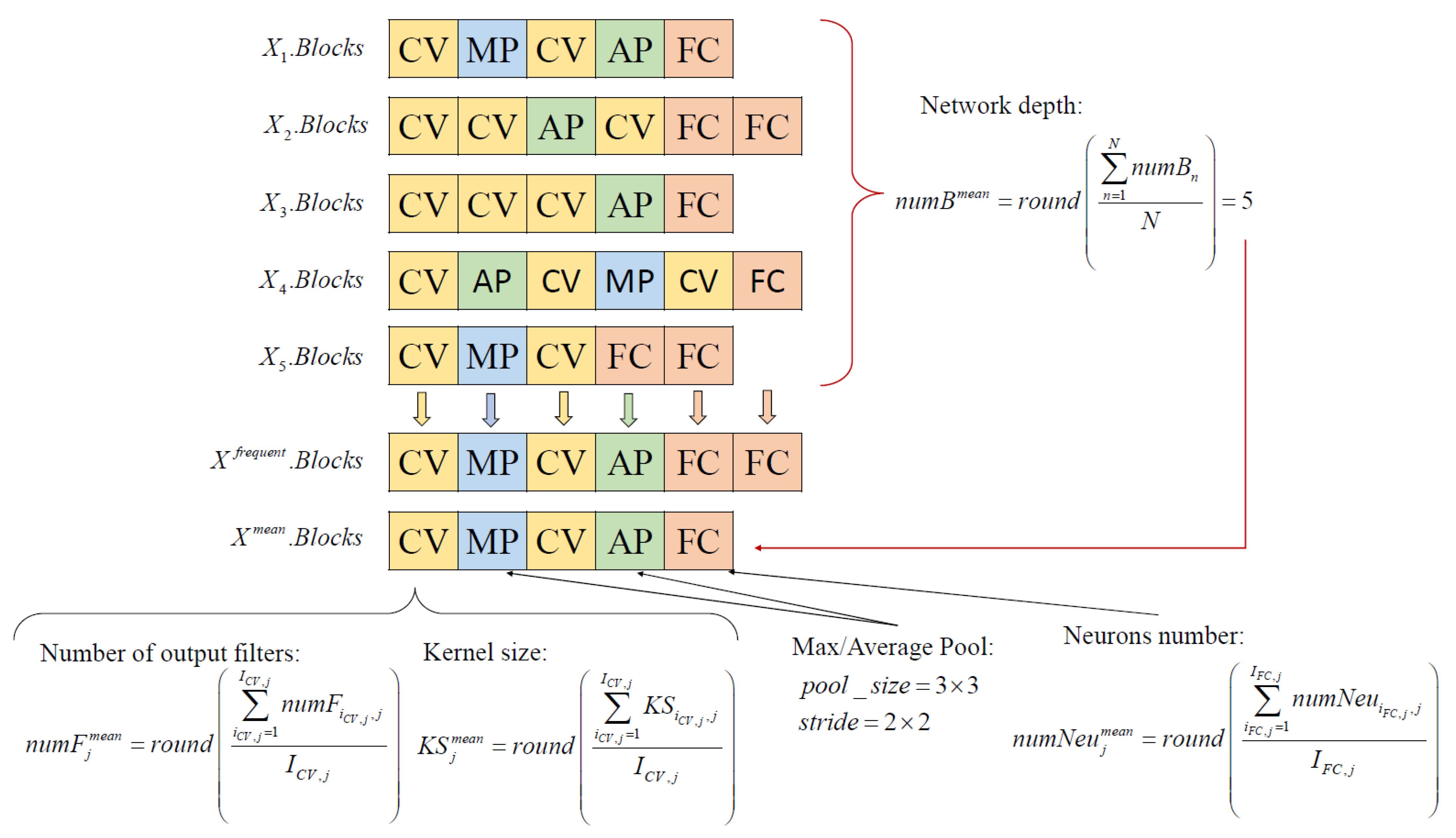
3.4.1. Computation of Mainstream CNN Architecture

In the teacher phase of original TLBO, the population mean (i.e., $X^{mean}$) is calculated using Equation (1) to describe the mainstream knowledge used to guide the population search and to update the new solutions of learners. It is non-trivial to calculate the population mean of TLBOCNN because the $X_n.Blocks$ of each nth learner has different lengths to represent a potential CNN model with unique architecture (in terms of network depth, layer types, kernel size, number of filters, number of neurons, etc.). A novel mechanism is introduced in the teacher phase of TLBOCNN to calculate the mainstream CNN architecture based on functional block information encoded in all learners with variable length.

Figure 3 shows the mechanisms used to construct a mainstream CNN architecture from the TLBOCNN population consisting of five learners (i.e., N = 5) that represents CNN models with different architectures. Define $X_n.Blocks\left[j\right]$ as functional block information stored in the jth dimension of the nth TLBOCNN learner, where $n=1,\dots ,N$ and $j=1,\dots ,num{B}_n$. Let $X^{frequent}.Blocks\left[j\right]$ be a list variable used to record the most frequently occurring functional block in the jth dimension of all learners, where $j=1,\dots ,num{B}^{frequent}$ and $num{B}^{frequent}$ are the largest network depth in the current population, i.e.,

$$num{B}^{frequent}=max(num{B}_n|n=1,\dots ,N)$$

(8)

For instance, the second and fourth learners of the TLBOCNN population shown in Figure 3 have the largest network depth. Therefore, the total dimensional size of $X^{frequent}.Blocks$ is set as $num{B}^{frequent}=6$. Let $I_{CV,j}$, $I_{Ave,j}$, $I_{Max,j}$, and $I_{FC,j}$ be the frequencies of convolutional block, average pooling block, maximum pooling block, and fully connected block occurring in the jth dimension, respectively, where $j=1,\dots ,num{B}^{frequent}$. For every jth dimension, the functional block with the highest frequency of occurrence is assigned to $X^{frequent}.Blocks\left[j\right]$. As shown in Figure 3, the average pooling block has the highest frequency of occurrence of $I_{Ave,j}=2$ for $j=4$, whereas the fully connected block appears most frequently at $j=5$ with $I_{FC,j}=4$. Therefore, the average pooling block and fully connected block are assigned to $X^{frequent}.Blocks\left[4\right]$ and $X^{frequent}.Blocks\left[5\right]$, respectively. For any jth dimension with more than one functional block appears with the highest frequency, such as $I_{Max,j}=I_{CV,j}=2$ for $j=2$. As shown in Figure 3, random selection is performed to choose one of these most frequently appearing functional blocks for the corresponding component of $X^{frequent}.Blocks\left[j\right]$. Referring to $X^{frequent}.Blocks$, the mainstream CNN architecture used for guiding the population search of TLBOCNN is then derived as $X^{mean}.Blocks$. Suppose that $num{B}^{mean}$ is the network depth of mainstream CNN architecture represented by $X^{mean}.Blocks$ and that it is calculated as:

$$num{B}^{mean}=round\left(\frac{{{\displaystyle \sum }}_{n=1}^{N}num{B}_n}{N}\right)$$

(9)

where $num{B}_n$ is the network depth of the CNN model represented by the nth TLBOCNN learner via $X_n.Blocks$; $round\left(·\right)$ is a rounding operator. According to Equations (8) and (9), $num{B}^{mean}\le num{B}^{frequent}$. The mainstream CNN architecture of $X^{mean}.Blocks$ is obtained by extracting the first $num{B}^{mean}$ elements from $X^{frequent}.Blocks$, i.e.,:

$$X^{mean}.Blocks\left[j\right]=X^{frequent}.Blocks\left[j\right],\mathrm{for}j=1,\dots ,num{B}^{mean}$$

(10)

Apart from the type of functional block to be assigned in every jth dimension of mainstream CNN architecture, i.e., $X^{mean}.Blocks\left[j\right]$, the hyperparameters of the selected functional block can also be calculated with the proposed mechanism. Supposing that a convolutional block is assigned to $X^{mean}.Blocks\left[j\right]$, the corresponding numbers of output filters (i.e., $num{F}_j^{mean}$) and kernel size (i.e., $K{S}_j^{mean}$) are calculated as:

$$num{F}_j^{mean}=round\left(\frac{{{\displaystyle \sum }}_{i_{CV,j}=1}^{I_{CV,j}}num{F}_{i_{CV,j},j}}{I_{CV,j}}\right)$$

(11)

$$K{S}_j^{mean}=round\left(\frac{{{\displaystyle \sum }}_{i_{CV,j}=1}^{I_{CV,j}}K{S}_{i_{CV,j},j}}{I_{CV,j}}\right)$$

(12)

where $i_{CV,j}=1,\dots ,I_{CV,j}$ refers to the index of a learner that is assigned as a convolutional block in the jth dimension; $I_{CV,j}$ is the frequency of convolutional blocks occurring in the j-th dimension. Meanwhile, if maximum pooling block or average pooling block is assigned to $X^{mean}.Blocks\left[j\right]$, their pool size and stride size are set as $3\times 3$ and $2\times 2$, respectively, according to Table 1. Finally, if a fully connected block is assigned to $X^{mean}.Blocks\left[j\right]$, the corresponding numbers of hidden neurons $numNe{u}_j^{mean}$ are calculated as:

$$numNe{u}_j^{mean}=round\left(\frac{{{\displaystyle \sum }}_{i_{FC,j}=1}^{I_{FC,j}}numNe{u}_{i_{FC,j},j}}{I_{FC,j}}\right)$$

(13)

where $i_{FC,j}=1,\dots ,I_{FC,j}$ refers to the index of learner that is assigned as fully connected block in the j th dimension; $I_{FC,j}$ is the frequency of the fully connected block occurring in the jth dimension. To satisfy the design constraints mentioned, the first (i.e., $j=1$) and last (i.e., $j=num{B}^{mean}$) blocks of mainstream CNN architecture are assigned to the convolutional and fully connected blocks, respectively. Furthermore, the number of output neurons assigned to the last fully connected block of mainstream CNN architecture in $X^{mean}.Blocks\left[num{B}^{mean}\right]$ is set equal to the numbers of output classes of datasets, i.e., $numNu{e}_{num{B}^{mean}}^{mean}=numOut$. The procedures used to generate the mainstream CNN architecture are summarized in Algorithm 3.

Algorithm 3: Computation of Mainstream CNN Architecture
Input:$P=\left\{X_1,\dots ,X_n,\dots ,X_N\right\}$, N, numOut
01:	$\mathrm{Calculate}num{B}^{frequent}$$\mathrm{using}\mathrm{Equation}\left(8\right)\mathrm{and}\mathrm{initialize}{X}^{frequent}.Blocks\leftarrow \varnothing$;
02:	forj$=1\mathrm{to}num{B}^{frequent}$do
03:		$\mathrm{Calculate}{I}_{CV,j}$$,I_{Ave,j}$$,I_{Max,j}$$\mathrm{and}{I}_{FC,j}$;
04:		if more than one functional block has highest frequency of occurrence do
05:			$\mathrm{Randomly}\mathrm{select}\mathrm{one}\mathrm{of}\mathrm{these}\mathrm{functional}\mathrm{blocks}\mathrm{and}\mathrm{assign}\mathrm{to}{X}^{frequent}.Blocks\left[j\right]$;
06:		else
07:			$\mathrm{Assign}\mathrm{the}\mathrm{functional}\mathrm{block}\mathrm{with}\mathrm{highest}\mathrm{frequency}\mathrm{of}\mathrm{occurrence}\mathrm{to}{X}^{frequent}.Blocks\left[j\right]$;
08:		end if
09:	end for
10:	$\mathrm{Calculate}num{B}^{mean}$$\mathrm{using}\mathrm{Equation}\left(9\right)\mathrm{and}\mathrm{initialize}{X}^{mean}.Blocks\leftarrow \varnothing$;
11:	forj$=1\mathrm{to}num{B}^{mean}$do
12:		ifj = 1 then
13:			$\mathrm{Assign}{X}^{mean}.Blocks\left[j\right]$ with convolutional block (CV);
14:			$\mathrm{Calculate}num{F}_j^{mean}$$\mathrm{and}K{S}_j^{mean}$ using Equations (11) and (12), respectively;
15:		else ifj =$num{B}^{mean}$do
16:			$\mathrm{Assign}{X}^{mean}.Blocks\left[j\right]$ with fully-connected block (FC);
17:			Assign $numNe{u}_j^{mean}$ as numOut;
18:		else ifj$>1\mathrm{and}j<num{B}^{mean}-1$then
19:			if$I_{CV,j}$ has the highest count then
20:				$\mathrm{Assign}{X}^{mean}.Blocks\left[j\right]$ with convolutional block (CV);
21:				$\mathrm{Calculate}num{F}_j^{mean}$$\mathrm{and}K{S}_j^{mean}$ using Equations (11) and (12), respectively;
22:			else if$I_{Max,j}$ has the highest count then
23:				$\mathrm{Assign}{X}^{mean}.Blocks\left[j\right]$ with maximum pooling block (MP);
24:				Set the $\mathrm{pool}\mathrm{size}\mathrm{and}\mathrm{stride}\mathrm{size}\mathrm{as}3\times 3$$\mathrm{and}2\times 2$, respectively;
25:			else if$I_{Ave,j}$ has the highest count then
26:				$\mathrm{Assign}{X}^{mean}.Blocks\left[j\right]$ with average pooling block (AP);
27:				Set the $\mathrm{pool}\mathrm{size}\mathrm{and}\mathrm{stride}\mathrm{size}\mathrm{as}3\times 3$$\mathrm{and}2\times 2$, respectively;
28:			else if$I_{FC,j}$ has the highest count then
29:				$\mathrm{Assign}{X}^{mean}.Blocks\left[j\right]$ with fully-connected block (FC);
30:				$\mathrm{Calculate}numNe{u}_j^{mean}$ using Equation (13);
31:			end if
32:		end if
33:	end for
Output:$X^{mean}.Blocks$

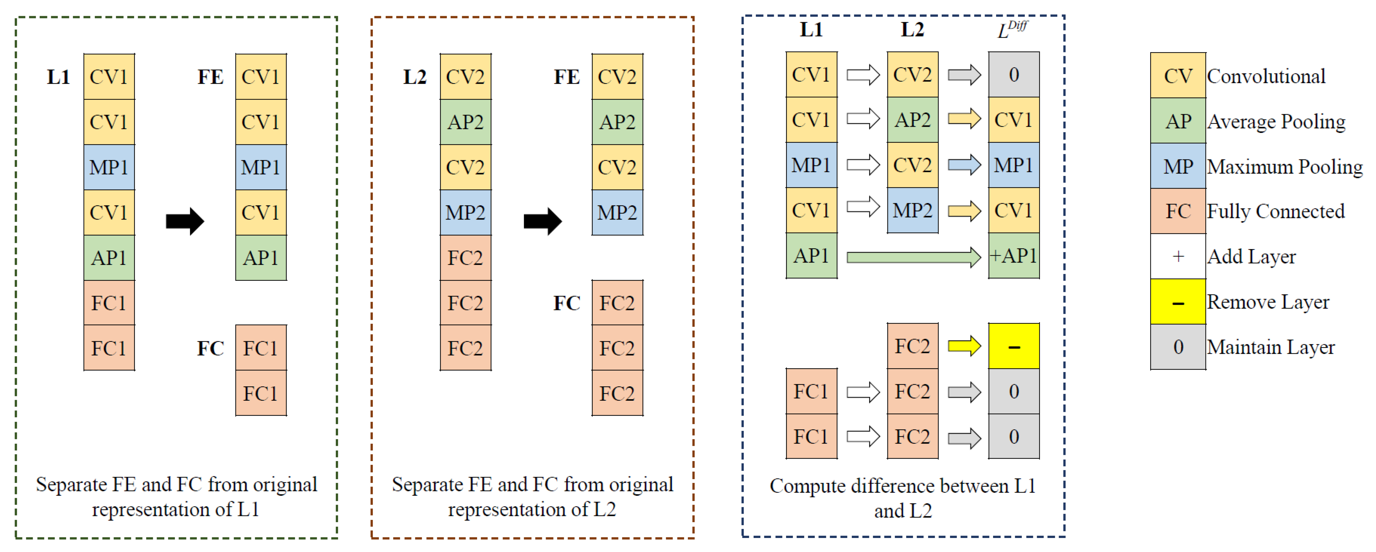
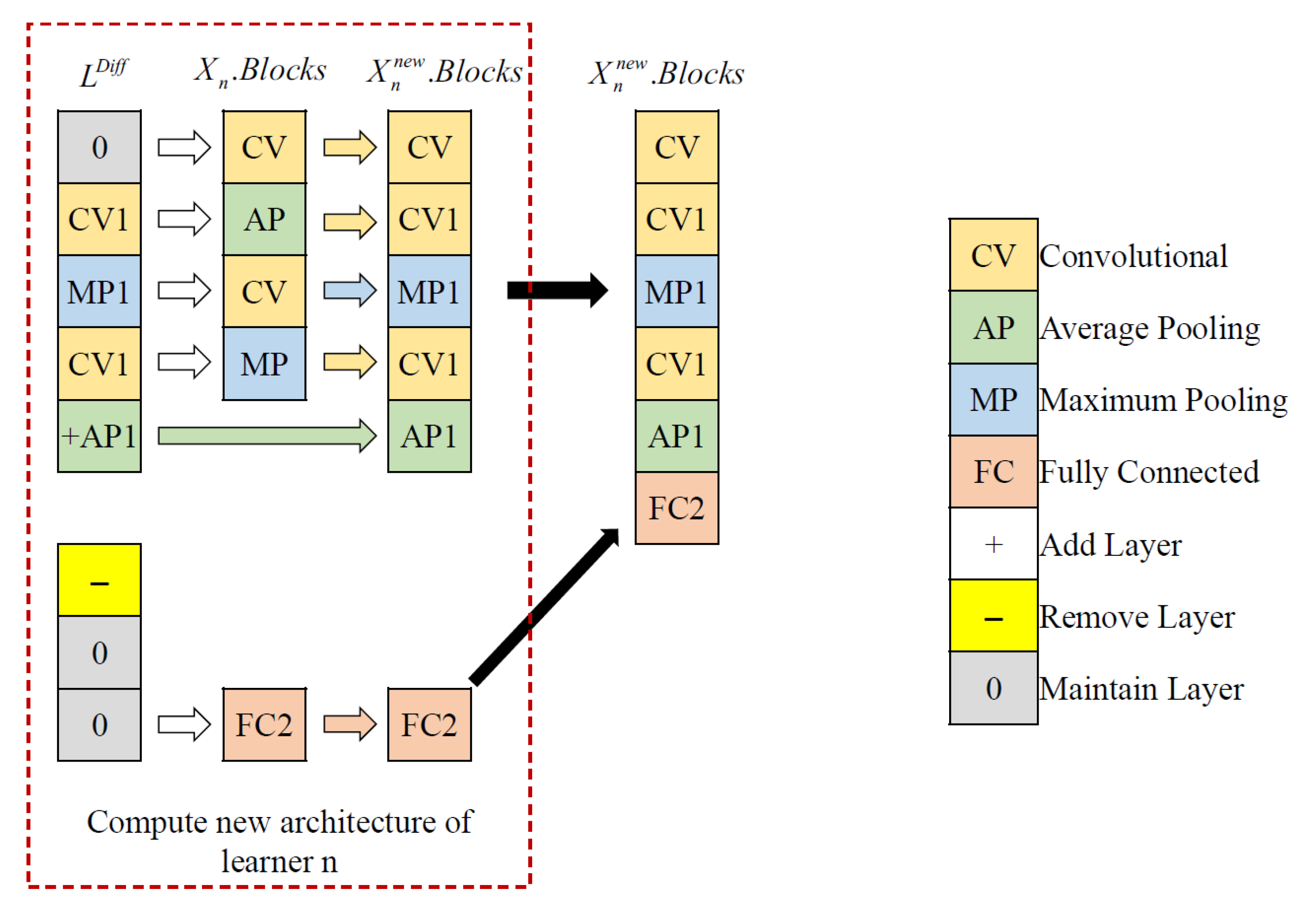
3.4.2. Computation of Differences between Two Learners

For the teacher phase in the original TLBO described in Equation (2), a new solution $X_n^{new}$ of each nth learner is updated based on the differences between the teacher solution $X^{teacher}$ and the mainstream knowledge of population $X^{mean}$. It is not trivial to determine the differences between CNN models represented by the teacher solution (i.e., $X^{teacher}.Blocks$) and mainstream CNN architecture (i.e., $X^{mean}.Blocks$) of TLBOCNN because they tend to have different network architectures (in terms of network depth, layer types, kernel size, number of filters, number of neurons, etc.). Furthermore, the information encoded in each dimension of $X^{teacher}.Blocks$ and $X^{mean}.Blocks$ refers to the functional block types (i.e., CV, MP, AP, and FC), which cannot be directly subtracted from each other.

Figure 4 illustrates the overall mechanisms used to measure the differences between CNN architectures represented by two TLBOCNN learners with variable lengths. Define L1 and L2 as two temporary list variables used to store the functional block information of $X^{teacher}.Blocks$ and $X^{mean}.Blocks$, respectively. The feature extraction module (i.e., FE) and fully connected layers (i.e., FC) of L1 and L2 are compared separately to ensure that the new CNN architectures obtained can comply to design constraints, i.e., the fully connected block cannot be inserted between the convolutional and pooling blocks within the feature extraction module. Let $L^{Diff}$ be a list variable used to store the differences between L1 and L2 (i.e., $L1-L2$); it has the total dimensional size of $num{B}^{Diff}$, calculated as:

$$num{B}^{Diff}=max(num{B}_{L1}^{FE},num{B}_{L2}^{FE})+max(num{B}_{L1}^{FC},num{B}_{L2}^{FC})$$

(14)

where $num{B}_{L1}^{FE}$ and $num{B}_{L2}^{FE}$ represent the total numbers of convolutional and pooling layers encoded in the feature extractor modules of L1 and L2, respectively, and $num{B}_{L1}^{FC}$ and $num{B}_{L2}^{FC}$ represent the total numbers of fully connected layers encoded in L1 and L2, respectively. For instance, Figure 4 shows that learner L1 has five convolutional and pooling layers in its feature extractor module (i.e., $num{B}_{L1}^{FE}=5$) and two fully connected layers (i.e., $num{B}_{L1}^{FC}=2$). Meanwhile, learner L2 has four convolutional and pooling layers in its feature extractor module (i.e., $num{B}_{L2}^{FE}=4$) and three fully connected layers (i.e., $num{B}_{L2}^{FC}=3$). Therefore, the list variable $L^{Diff}$ used to store the differences between L1 and L2 has the total dimensional size of $num{B}^{Diff}=8$ according to Equation (14).

The following guidelines are used to compare the differences between CNN architectures encoded in every jth dimension of learners L1 and L2 and stored in $L^{Diff}\left[j\right]$, where $j=1,\dots ,num{B}^{Diff}$. When both L1 and L2 have different functional block types encoded in the jth dimension, the information contained in $L1\left[j\right]$ (i.e., functional block type and its hyperparameters) are extracted and assigned to $L^{Diff}\left[j\right]$. For instance, if $L1\left[j\right]=‘CV’$ and $L2\left[j\right]=‘AP’$, then the jth dimension of $L^{Diff}$ is assigned with the convolutional block, i.e., $L^{Diff}\left[j\right]=‘CV’$, along with its hyperparameters. $L^{Diff}\left[j\right]$ is assigned as ‘0’ when both L1 and L2 have same functional block type encoded in the jth dimension, implying that there are no changes in functional block in this dimension when it is used to calculate the CNN architecture of a new learner. When comparing L1 and L2 with different network depths, it is possible for L1 to have more functional blocks than L2 or vice versa. For any jth dimension, if L1 has more functional blocks than L2 in the feature selector module or the fully connected layer, $L^{Diff}\left[j\right]$ is assigned as ‘+B’ to imply that a new functional block should be added by referring to that of $L1\left[j\right]$, where B can refer to CV, AP, MP, or FC blocks. On the other hand, $L^{Diff}\left[j\right]$ is assigned as ‘-’ to indicate the removal of an existing functional block when L1 has lesser functional block than L2 in the jth dimension of the feature selector module or the fully connected layer. The overall procedures used to compare the differences between L1 and L2 are summarized in Algorithm 4.

Algorithm 4: Calculate Differences Between L1 and L2
Input:L1, L2
01:	Separate the FC layers encoded in L1 and L2 from the FE module as shown in Figure 4.
02:	$\mathrm{Calculate}num{B}_{L1}^{FE}$$\mathrm{and}num{B}_{L1}^{FC}$$\mathrm{from}L1\mathrm{as}\mathrm{well}\mathrm{as}num{B}_{L2}^{FC}$$\mathrm{and}num{B}_{L2}^{FC}$ from L2;
03:	$\mathrm{Calculate}num{B}^{Diff}$$\mathrm{using}\mathrm{Equation}\left(14\right)\mathrm{and}\mathrm{initialize}{L}^{Diff}\leftarrow \varnothing$;;
04:	forj$=1\mathrm{to}num{B}^{Diff}$do
05:		if$L1\left[j\right]$$\mathrm{has}\mathrm{different}\mathrm{functional}\mathrm{block}\mathrm{with}L2\left[j\right]$then
06:			$\mathrm{Assign}{L}^{Diff}\left[j\right]$$\mathrm{with}\mathrm{the}\mathrm{functional}\mathrm{block}\mathrm{information}\mathrm{of}L1\left[j\right]$;
07:		else if$L1\left[j\right]$$\mathrm{has}\mathrm{same}\mathrm{functional}\mathrm{block}\mathrm{with}L2\left[j\right]$then
08:			$\mathrm{Assign}{L}^{Diff}\left[j\right]$ with ‘0’ to indicate no changes of functional block;
09:		else if$L1\left[j\right]$$\mathrm{has}\mathrm{functional}\mathrm{block}\mathrm{and}L2\left[j\right]$ has no functional block then
10:			$\mathrm{Assign}{L}^{Diff}\left[j\right]$$\mathrm{with}‘+B’,\mathrm{where}B\mathrm{refers}\mathrm{to}\mathrm{the}\mathrm{functional}\mathrm{block}\mathrm{information}\mathrm{obtained}\mathrm{from}L1\left[j\right]$;
11:		else if$L1\left[j\right]$$\mathrm{has}\mathrm{no}\mathrm{functional}\mathrm{block}\mathrm{and}L2\left[j\right]$ has functional block then
12:			$\mathrm{Assign}{L}^{Diff}\left[j\right]$ with ‘-’ to indicate the removal of functional block;
13:		end if
14:	end for
Output:$L^{Diff}$

3.4.3. Computation of New Learner

Given the difference $L^{Diff}$ obtained between $X^{teacher}.Blocks$ and $X^{mean}.Blocks$ from Algorithm 4, a new learner with CNN representation of $X_n^{new}.Blocks$ is calculated for every nth TLBOCNN learner with a CNN representation of $X_n.Blocks$. The position update mechanism of the original TLBO stated in Equation (2) is not applicable to calculating the new $X_n^{new}.Blocks$ from $L^{Diff}$ and $X_n.Blocks$ due to their different network depths and the infeasibility of direct subtraction between functional blocks. Figure 5 illustrates the overall mechanisms used to calculate the new solution of n-th learner (i.e., $X_n^{new}.Blocks$) based on its current solution (i.e., $X_n.Blocks$) and the differences between teacher solution and population mean (i.e., $L^{Diff}$). Similarly, the feature extraction module (i.e., FE) and fully connected layers (i.e., FC) of $L^{Diff}$ and $X_n.Blocks$ are compared independently to ensure the new CNN architectures obtained in $X_n^{new}.Blocks$ can comply to design constraint, i.e., a fully connected block cannot be inserted between the convolutional and pooling blocks within feature extraction module. Define $num{B}_n^{new,max}$ as the maximum dimensional size of $X_n^{new}.Blocks$ and it is calculated as:

$$num{B}_n^{new,max}=\max \left(num{B}_{Diff}^{FE},num{B}_n^{FE}\right)+\max \left(um{B}_{Diff}^{FC},num{B}_n^{FC}\right)$$

(15)

where $num{B}_{Diff}^{FE}$ and $num{B}_n^{FE}$ are the total numbers of convolutional and pooling layers encoded in $L^{Diff}$ and $X_n.Blocks$, respectively; $num{B}_{Diff}^{FC}$ and $num{B}_n^{FC}$ are the total numbers of fully connected layers encoded in $L^{Diff}$ and $X_n.Blocks$, respectively.

The following guidelines are used to determine the functional block information assigned to each jth dimension of $X_n^{new}.Blocks$ by comparing those of $L^{Diff}$ and $X_n.Blocks$, where $j=1,\dots ,num{B}_n^{new,max}$. If $L^{Diff}\left[j\right]$ is assigned as ‘0’ and $X_n.Blocks\left[j\right]$ is not empty, then $X_n^{new}.Blocks\left[j\right]$ can inherit the functional block and hyperparameters of $X_n^{new}.Blocks\left[j\right]$. For instance, if $L^{Diff}\left[j\right]=0$ and $X_n.Blocks\left[j\right]=‘CV’$, then the jth dimension of $X_n^{new}.Blocks$ is assigned as a convolutional block, i.e., $X_n^{new}.Blocks\left[j\right]=‘CV’$ along with its hyperparameters. On the other hand, $X_n^{new}.Blocks\left[j\right]$ is assigned as an empty value if $L^{Diff}\left[j\right]$ is assigned as ‘0’ and $X_n.Blocks\left[j\right]$ is empty. If $L^{Diff}\left[j\right]$ is assigned as “-”, then $X_n^{new}.Blocks\left[j\right]$ is also assigned as an empty value regardless of the presence of any functional block in $X_n.Blocks\left[j\right]$. When $L^{Diff}\left[j\right]$ is assigned “+B” where B can refer to the functional blocks of Conv, AP, MP, or FC, $X_n^{new}.Blocks\left[j\right]$ is added with a new functional block as specified in B regardless of the presence of any functional block in $X_n.Blocks\left[j\right]$. For instance, if $L^{Diff}\left[j\right]=‘+AP’$ and $X_n.Blocks\left[j\right]$ is an empty value, then an average pooling block is added to $X_n^{new}.Blocks\left[j\right]$. It is also notable that $X_n^{new}.Blocks\left[j\right]$ always refers to the functional block assigned in $L^{Diff}\left[j\right]$ without considering the presence of any functional block in $X_n.Blocks\left[j\right]$. On the other hand, $X_n^{new}.Blocks\left[j\right]$ only refers to the functional block of $X_n.Blocks\left[j\right]$ if $L^{Diff}\left[j\right]$ is an empty value. Algorithm 5 presents the pseudocode used to calculate $X_n^{new}.Blocks$ based on $L^{Diff}$ and $X_n.Blocks$. For any $X_n^{new}.Blocks\left[j\right]$ assigned with an empty value in the jth dimension, it implies the absence of functional block information and can be eliminated. The numbers of AP and MP blocks contained in $X_n^{new}.Blocks$ must be adjusted based on the input sizes of datasets. Excessive pooling layers must be removed from $X_n^{new}.Blocks$ one by one starting from the last layer if the new solution of the nth learner is found to have more pooling layers than allowed by the sizes of input datasets. Therefore, the actual dimensional size of $X_n^{new}.Blocks$ (i.e., $num{B}_n^{new,actual}$) can be smaller than that of $num{B}_n^{new,max}$ obtained from Equation (15) after these post-processing processes.

Algorithm 5:$\mathrm{Calculate}\mathrm{New}\mathrm{Solution}\mathrm{Based}\mathrm{on}{L}^{Diff}$$\mathrm{and}{X}_n.Blocks$
Input: Functional block information encoded in $L^{Diff}$$\mathrm{and}{X}_n.Blocks$
01:	$\mathrm{Separate}\mathrm{the}\mathrm{FC}\mathrm{layers}\mathrm{encoded}\mathrm{in}{L}^{Diff}$$\mathrm{and}{X}_n.Blocks$ from the FE module as shown in Figure 5.
02:	$\mathrm{Calculate}num{B}_{Diff}^{FE}$$\mathrm{and}num{B}_{Diff}^{FC}$$\mathrm{from}{L}^{Diff}$$\mathrm{as}\mathrm{well}\mathrm{as}num{B}_n^{FC}$$\mathrm{and}num{B}_n^{FC}$$\mathrm{from}{X}_n.Blocks$;
03:	$\mathrm{Calculate}num{B}_n^{new,max}$$\mathrm{using}\mathrm{Equation}\left(15\right)\mathrm{and}\mathrm{initialize}{X}_n^{new}.Blocks\leftarrow \varnothing$;
04:	forj$=1\mathrm{to}num{B}_n^{new,max}$do
05:		if$L^{Diff}\left[j\right]=‘0’$$\mathrm{and}{X}_n.Blocks\left[j\right]$ has a functional block then
06:			$\mathrm{Assign}{X}_n^{new}.Blocks\left[j\right]$$\mathrm{with}\mathrm{the}\mathrm{functional}\mathrm{block}\mathrm{information}\mathrm{of}{X}_n.Blocks\left[j\right]$;
07:		else if$L^{Diff}\left[j\right]=‘0’$$\mathrm{and}{X}_n.Blocks\left[j\right]$ has no functional block then
08:			$\mathrm{Assign}{X}_n^{new}.Blocks\left[j\right]$ with an empty value;
09:		else if$L^{Diff}\left[j\right]=‘-’$then
10:			$\mathrm{Assign}{X}_n^{new}.Blocks\left[j\right]$ with an empty value;
11:		else if$L^{Diff}\left[j\right]=‘+B’$then
12:			$\mathrm{Assign}{X}_n^{new}.Blocks\left[j\right]$ with the functional block information of B;
13:		else if$L^{Diff}\left[j\right]$ has a functional block then
14:			$\mathrm{Assign}{X}_n^{new}.Blocks\left[j\right]$$\mathrm{with}\mathrm{the}\mathrm{functional}\mathrm{block}\mathrm{information}\mathrm{of} L^{Diff}\left[j\right]$;
15:		else if$L^{Diff}\left[j\right]$$\mathrm{has}\mathrm{no}\mathrm{functional}\mathrm{block}\mathrm{and}{X}_n.Blocks\left[j\right]$ has a functional block then
16:			$\mathrm{Assign}{X}_n^{new}.Blocks\left[j\right]$$\mathrm{with}\mathrm{the}\mathrm{functional}\mathrm{block}\mathrm{information}\mathrm{of}{X}_n.Blocks\left[j\right]$;
17:		end if
18:	end for
19:	$\mathrm{Eliminate}\mathrm{the}\mathrm{dimensional}\mathrm{component}\mathrm{of}{X}_n^{new}.Blocks$ assigned with an empty value;
20:	$\mathrm{Reduce}\mathrm{the}\mathrm{pooling}\mathrm{layers}\mathrm{in} X_n^{new}.Blocks$ one by one starting from last layers if it is found to have more pooling layers than that allowed by the sizes of input datasets.
Output:$X_n^{new}.Blocks$;

The overall mechanisms of the teacher phase in TLBOCNN are described in Algorithm 6. After obtaining the new solution of the nth learner (i.e.,$X_n^{new}.Blocks$) via the teacher phase, the fitness of this new solution is evaluated using Algorithm 2 to measure its classification accuracy $X_n^{new}.Acc$, which is compared to that of $X_n.Blocks$ (i.e., $X_n.Acc$). If the CNN architecture represented by $X_n^{new}.Blocks$ has better fitness than $X_n.Blocks$ does, i.e., $X_n^{new}.Acc>X_n.Acc$, the new solution of the nth TLBOCNN learner can be used to replace its current solution. Otherwise, the more inferior new solution is discarded and the original solution of the nth learner is retained. A similar mechanism is used to determine if the new solution obtained by every nth learner can be used to replace the teacher solution.

Algorithm 6: Teacher Phase of TLBOCNN
Input:$P=\left\{X_1,\dots ,X_n,\dots ,X_N\right\}$$,N,X^{teacher}$, $Dat{a}_{train}$, $Dat{a}_{valid}$, $batch\_size$$,e_{train}$, $\ell$, $numOut$
01:	$\mathrm{Compute}{X}^{mean}.Blocks$ with Algorithm 3;
02:	forn = 1 to N do
03:		$L1\leftarrow X^{teacher}.Blocks$, $L2\leftarrow X^{mean}.Blocks$;
04:		$\mathrm{Calculate}{L}^{Diff}$ from L1 and L2 with Algorithm 4;
03:		$\mathrm{Calculate}{X}_n^{new}.Blocks$ based on $L^{Diff}$$\mathrm{and}{X}_n.Blocks$ with Algorithm 5;
04:		$\mathrm{Perform}\mathrm{fitness}\mathrm{evaluation}\mathrm{on} X_n^{new}.Blocks$ to obtain $X_n^{new}.Acc$ with Algorithm 2;
06:		if$X_n^{new}.Acc$ $\mathrm{is}\mathrm{higher}\mathrm{than}{X}_n.Acc$then
07:			$X_n.Blocks\leftarrow X_n^{new}.Blocks$, $X_n.Acc\leftarrow X_n^{new}.Acc$;
08:			if $X_n^{new}.Acc$ $\mathrm{is}\mathrm{higher}\mathrm{than}{X}^{teacher}.Acc$ then
09:			$X^{teacher}.Blocks\leftarrow X_n^{new}.Blocks$, $X^{teacher}.Acc\leftarrow X_n^{new}.Acc$;
10:			end if
11:		end if
12:	end for
Output:$P=\left\{X_1,\dots ,X_n,\dots ,X_N\right\}$$,X^{teacher}$

3.5. Learner Phase of TLBOCNN

The learner phase of TLBOCNN facilitates information exchange between the peer learners to update their solutions. For each nth TLBOCNN learner with a CNN representation of $X_n.Blocks$, its new CNN architecture represented in $X_n^{new}.Blocks$ can be obtained by interacting with a randomly selected pth peer learner with a CNN representation of $X_p.Blocks$, where $n\ne p$. Similarly to the teacher phase, the original position update mechanism used in the learner phase of TLBO as described in Equation (3) cannot be used to determine the new $X_n^{new}.Blocks$ of the nth TLBOCNN learner from $X_n.Blocks$ and $X_p.Blocks$ due to their different network depths and the infeasibility of direct subtraction of functional blocks.

Algorithm 7 presents the overall mechanisms used to calculate new CNN representation $X_n^{new}.Blocks$ of every nth learner in the learner phase of TLBOCNN. Suppose that $X_n.Acc$ and $X_p.Acc$ refer to the fitness values of the nth learner and pth learner in terms of the classification accuracies achieved by their respective CNN models. If the CNN model represented by the pth peer learner has higher classification accuracy than the nth learner does, i.e., $X_p.Acc>X_n.Acc$, their CNN representations of $X_p.Blocks$ and $X_n.Blocks$ are assigned to the temporary list variables of L1 and L2, respectively. On the other hand, $X_n.Blocks$ and $X_p.Blocks$ are stored in L1 and L2, respectively, if the CNN model represented by the pth peer learner does not have better classification accuracy than the nth learner, i.e.,$X_p.Acc\le X_n.Acc$. Referring to the functional block information encoded in both L1 and L2, their differences can be measured as $L^{Diff}$ by using Algorithm 4. Given $L^{Diff}$ and $X_n.Blocks$, the new CNN representation of the nth learner can be obtained as $X_n^{new}.Blocks$ with Algorithm 5. The fitness value of $X_n^{new}.Blocks$ is evaluated using Algorithm 2 to measure its classification accuracy $X_n^{new}.Acc$ and compared with that of $X_n.Blocks$ (i.e., $X_n.Acc$). If the new CNN architecture represented by $X_n^{new}.Blocks$ has better fitness than $X_n.Blocks$, i.e., $X_n^{new}.Acc>X_n.Acc$, the new solution of the nth TLBOCNN learner can be used to replace its current solution. Otherwise, the more inferior new solution is discarded and the original solution of the nth learner is retained. A similar mechanism is used to determine if the new solution obtained by every nth learner can be used to replace the teacher solution.

Algorithm 7: Learner Phase of TLBOCNN
Input:$P=\left\{X_1,\dots ,X_n,\dots ,X_N\right\}$$,N,X^{teacher}$, $Dat{a}_{train}$, $Dat{a}_{valid}$, $batch\_size$, $e_{train}$, $\ell$, $numOut$
01:	forn = 1 to N do
02:		$\mathrm{Randomly}\mathrm{selected}\mathrm{the}p\mathrm{th}\mathrm{peer}\mathrm{learner}\mathrm{from}\mathrm{population},\mathrm{where}p\ne n$;
03:		if$X_p.Acc$$\mathrm{is}\mathrm{higher}\mathrm{than}{X}_n.Acc$then
04:			$L1\leftarrow X_p.Blocks$$,L2\leftarrow X_n.Blocks$;
05:		else
06:			$L1\leftarrow X_n.Blocks$$,L2\leftarrow X_p.Blocks$;
07:		end if
08:		$\mathrm{Calculate}{L}^{Diff}$ from L1 and L2 with Algorithm 4;
09:		$\mathrm{Calculate}{X}_n^{new}.Blocks$ based on $L^{Diff}$ $\mathrm{and}{X}_n.Blocks$ with Algorithm 5;
10:		$\mathrm{Perform}\mathrm{fitness}\mathrm{evaluation}\mathrm{on} X_n^{new}.Blocks$ to obtain $X_n^{new}.Acc$ with Algorithm 2;
11:		if$X_n^{new}.Acc$ $\mathrm{is}\mathrm{higher}\mathrm{than} X_n.Acc$then
12:			$X_n.Blocks\leftarrow X_n^{new}.Blocks$, $X_n.Acc\leftarrow X_n^{new}.Acc$;
13:			if $X_n^{new}.Acc$ $\mathrm{is}\mathrm{higher}\mathrm{than}{X}^{teacher}.Acc$ then
14:			$X^{teacher}.Blocks\leftarrow X_n^{new}.Blocks$, $X^{teacher}.Acc\leftarrow X_n^{new}.Acc$;
15:			end if
16:		end if
17:	end for
Output:$P=\left\{X_1,\dots ,X_n,\dots ,X_N\right\}$$,X^{teacher}$

3.6. Overall Framework of TLBOCNN

The overall framework of the proposed TLBOCNN is presented in Algorithm 8, where $\upsilon$ is a counter variable used to record the current iteration number and ${\upsilon }^{max}$ is the maximum iteration number used as terminate criterion of TLBOCNN. After loading the training and validation datasets (i.e., $Dat{a}_{train}$ and $Dat{a}_{valid}$), the initial population of TLBOCNN is generated using Algorithm 1. The new CNN architectures represented by TLBOCNN learners are iteratively generated via the teacher phase (Algorithm 6) and the learner phase (Algorithm 7) until the termination criterion of $\upsilon >{\upsilon }^{max}$ is satisfied. After completing the search process, $X^{teacher}$ is returned as the best solution found by TLBOCNN. As explained in earlier subsection, the CNN architectures represented by all TLBOCNN learners are trained with a small epoch number of $e_{train}$ during the fitness evaluation process (Algorithm 2) to prevent excessive computational overhead of the proposed algorithm, but this approach cannot solve real-world applications with optimal performance. Therefore, a full training process with larger epoch numbers of $e_{train}^{full}$ is performed on the CNN architecture represented by $X^{teacher}.Blocks$ after TLBOCNN is terminated. It is noteworthy that the mechanisms of full training process are same as those of Algorithm 2 except that a larger $e_{train}^{full}$ is used to ensure the optimal performance of CNN architecture obtained. Dropout and batch normalization can be added between layers to address the overfitting issue. At the end of the full training process, information related to the fully trained CNN model represented by $X^{teacher}.Blocks$ (i.e., architecture, classification accuracy, and number of network parameters) is returned.

Algorithm 8: TLBOCNN
$\mathrm{Input}:Dat{a}_{train}$$,Dat{a}_{valid}$$,batch\_size$$,e_{train}$$,e_{train}^{full}$$,$,$\upsilon$, ${\upsilon }^{max}$, N, $num{B}^{min}$$,num{B}^{max}$$,num{F}^{min}$$,num{F}^{max}$$,KS$$,numNe{u}^{min}$$,numNe{u}^{max}$, numOut
01:	$\mathrm{Load}\mathrm{training}\mathrm{dataset}Dat{a}_{train}$$\mathrm{and}\mathrm{validation}\mathrm{dataset}Dat{a}_{valid}$ from the directory;
02:	$\mathrm{Population}\mathrm{initialization}\mathrm{of}P=\left\{X_1,\dots ,X_n,\dots ,X_N\right\}$ with Algorithm 1;
03:	$\mathbf{for}\upsilon$ $=1\mathrm{to}{\upsilon }^{max}$do
04:		$\mathrm{Perform}\mathrm{teacher}\mathrm{phase}\mathrm{to}\mathrm{update}P$$\mathrm{and}{X}^{teacher}$ with Algorithm 6;
05:		$\mathrm{Perform}\mathrm{learner}\mathrm{phase}\mathrm{to}\mathrm{update}P$$\mathrm{and}{X}^{teacher}$ with Algorithm 7;
06:	end for
07:	$\mathrm{Perform}\mathrm{full}\mathrm{training}\mathrm{on}\mathrm{the}\mathrm{best}\mathrm{CNN}\mathrm{architecture}\mathrm{of}{X}^{teacher}.Blocks$$\mathrm{with}{e}_{train}^{full}$ using Algorithm 2;
08:	$\mathrm{Calculate}\mathrm{the}\mathrm{numbers}\mathrm{of}\mathrm{network}\mathrm{parameters}\mathrm{of}\mathrm{fully}-\mathrm{trained}\mathrm{best}\mathrm{CNN}\mathrm{architecture}\mathrm{represented}\mathrm{by}{X}^{teacher}.Blocks$$\mathrm{and}\mathrm{stored}\mathrm{as}{X}^{teacher}.Params$;
$\mathbf{Output}:X^{teacher}$

4. Experimental Design and Results Analysis

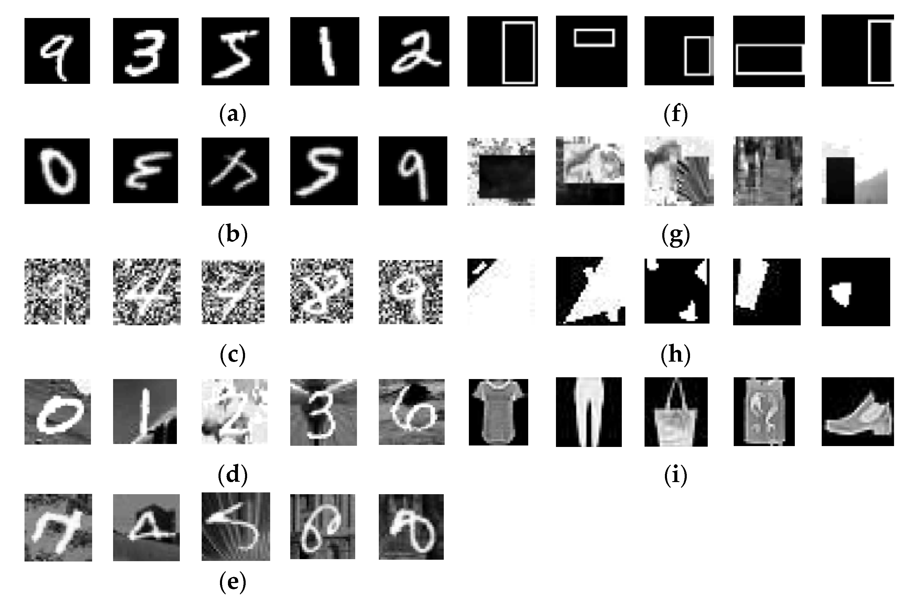
4.1. Image Datasets

In this section, the classification performance of the proposed TLBOCNN algorithm is evaluated by using nine image datasets with different characteristics and compared to state-of-the-art peer classifiers. The selected image datasets are Modified National Institute of Standards and Technology (MNIST), MNIST with Rotated Digits (MNIST-RD), MNIST with Random Background (MNIST-RB), MNIST with Background Images (MNIST-BI), MNIST with Rotated Digits and Background Images (MNIST-RD+BI), Rectangles, Rectangles with Images (Rectangles-I), Convex, and Fashion. These image datasets are publicly available at http://www.iro.umontreal.ca/~lisa/icml2007data/ (accessed on 3 June 2022), while the sample images of each selected dataset with a size of $28\times 28$ are illustrated in Figure 6. Meanwhile,

Table 2. Overview of the image datasets used for performance evaluation of TLBOCNN.

Dataset	Input Size	No. of Output Classes	No. of Training Samples	No. of Testing Samples
MNIST	$28\times 28\times 1$	10	50,000	10,000
MNIST-RD	$28\times 28\times 1$	10	12,000	50,000
MNIST-RB	$28\times 28\times 1$	10	12,000	50,000
MNIST-BI	$28\times 28\times 1$	10	12,000	50,000
MNIST-RD+BI	$28\times 28\times 1$	10	12,000	50,000
Rectangles	$28\times 28\times 1$	2	1200	50,000
Rectangles-I	$28\times 28\times 1$	2	12,000	50,000
Convex	$28\times 28\times 1$	2	8000	50,000
Fashion	$28\times 28\times 1$	10	60,000	10,000

summarizes the characteristics of nine selected image classification benchmark datasets in terms of their input size, number of output classes, numbers of training samples, and numbers of testing samples.

MNIST [55] is a popular image dataset used to test classification performance of machine learning or deep learning algorithms. Different mechanisms, such as rotation, random background noise, background images, and combinations of rotation and background images are introduced into original MNIST to produce MNIST-RD, MNIST-RB, MNIST-BI, and MNIST-RD+BI, respectively [77]. These MNIST variants contain irrelevant information and are useful for evaluating the generalization capability of classifiers. The Rectangle dataset is a collection of grayscale images of rectangle outlines with different sizes, and it aims to train the machine learning or deep learning models to recognize the larger dimension of rectangles (i.e., height or width). Rectangle with Image (Rectangle-I) dataset is more challenging because it requires the trained models to identity if the images patches are located inside the rectangle or the background of images. The Convex dataset is a collection of grayscale geometrical shape images, and the models are trained to recognize if the geometrical shape is convex or non-convex. The Fashion dataset [78] contains the grayscale image collection of fashion products that can be categorized into 10 output classes: trousers, dresses, coats, top, bags, sneakers, sandals, ankle boots, pullovers, and shirts. It is considered to be a more challenging dataset and is used to benchmark the classification performances of machine learning and deep learning algorithms.

4.2. Selection of Peer Algorithms and Simulation Settings

The well-established machine learning and deep learning models that have solved the nine selected datasets with promising classification accuracy are selected as the peer algorithms of the proposed TLBOCNN. In particular, 13 peer algorithms—RandNet-2 [79], LDANet-2 [79], CAE-1 [80], CAE-2 [80], ScatNet-2 [81], SVM+RBF [77], SVM+Poly [77], PCANet-2 [79], NNet [77], SAA-3 [77], DBN-3 [77], EvoCNN [67], and psoCNN [60]—are chosen for performance-comparative studies with TLBOCNN in solving eight datasets: MNIST, MNIST-RD, MNIST-RB, MNIST-RI, MNIST-RD+BI, Rectangle, Rectangle-I, and Convex. Another 15 peer algorithms compared to TLBOCNN for the Fashion dataset were AlexNet [22], VGG [23], ResNet [25], SqueezeNet-200 [82], EvoCNN [67], psoCNN [60], 2C1P2F+Dropout, 2C1P2F, 3C2F, 3C1P2F + Dropout, GRU+SVM, GRU+SVM+Dropout, HOG+SVM, MLP 256-128-64, and MLP 256-128-100. The results of all peer algorithms are either extracted from the literature (e.g., https://github.com/zalandoresearch/fashion-mnist (accessed on 3 June 2022)) or simulated based on the original source codes provided by their authors. Notably, EvoCNN [67] and psoCNN [60] are the only metaheuristic-search-based algorithms that share similar concepts with the proposed TLBOCNN, i.e., the best network architectures for given datasets are searched iteratively until termination criteria are satisfied. All parameter settings of TLBOCNN are presented in

Table 3. Parameter settings of proposed TLBOCNN for performance analyses.

Parameters	Values
$\mathrm{Maximum}\mathrm{iteration}\mathrm{number},{\upsilon }^{max}$	10
Population size, N	20
$\mathrm{Minimum}\mathrm{total}\mathrm{number}\mathrm{of}\mathrm{layers},nLaye{r}^{min}$	3
$\mathrm{Maximum}\mathrm{total}\mathrm{number}\mathrm{of}\mathrm{layers},nLaye{r}^{max}$	20
$\mathrm{Minimum}\mathrm{number}\mathrm{of}\mathrm{filters}\mathrm{of}\mathrm{convolution}\mathrm{layer},nFilte{r}^{min}$	3
$\mathrm{Maximum}\mathrm{number}\mathrm{of}\mathrm{filters}\mathrm{of}\mathrm{convolution}\mathrm{layer},nFilte{r}^{max}$	256
$\mathrm{Minimum}\mathrm{kernel}\mathrm{size}\mathrm{of}\mathrm{of}\mathrm{convolution}\mathrm{layer},nK{S}^{min}$	$3\times 3$
$\mathrm{Maximum}\mathrm{kernel}\mathrm{size}\mathrm{of}\mathrm{of}\mathrm{convolution}\mathrm{layer},nK{S}^{max}$	$7\times 7$
Pool size of pooling layer	$3\times 3$
Stride size of pooling layer	$2\times 2$
$\mathrm{Minimum}\mathrm{number}\mathrm{of}\mathrm{neurons}\mathrm{of}\mathrm{fully}\mathrm{connected}\mathrm{layer},nNe{u}^{min}$	1
$\mathrm{Maximum}\mathrm{number}\mathrm{of}\mathrm{neurons}\mathrm{of}\mathrm{fully}\mathrm{connected}\mathrm{layer},nNe{u}^{max}$	300
Batch normalization	Yes
Dropout rate	0.5
$\mathrm{Number}\mathrm{of}\mathrm{epochs}\mathrm{for}\mathrm{learner}\mathrm{evaluation}\mathrm{during}\mathrm{optimization},e_{train}$	1
$\mathrm{Number}\mathrm{of}\mathrm{epochs}\mathrm{for}\mathrm{full}\mathrm{training}\mathrm{of}\mathrm{teacher}\mathrm{solution},e_{train}^{full}$	100

, and their values are chosen based on the conventions of deep learning and MSA communities. Simulations of TLBOCNN are conducted for 30 independent runs on a personal computer installed with Python 3.8.5 and an Nvidia GeForce RTX 3090 to obtain statistically meaningful results.

4.3. Simulation Results

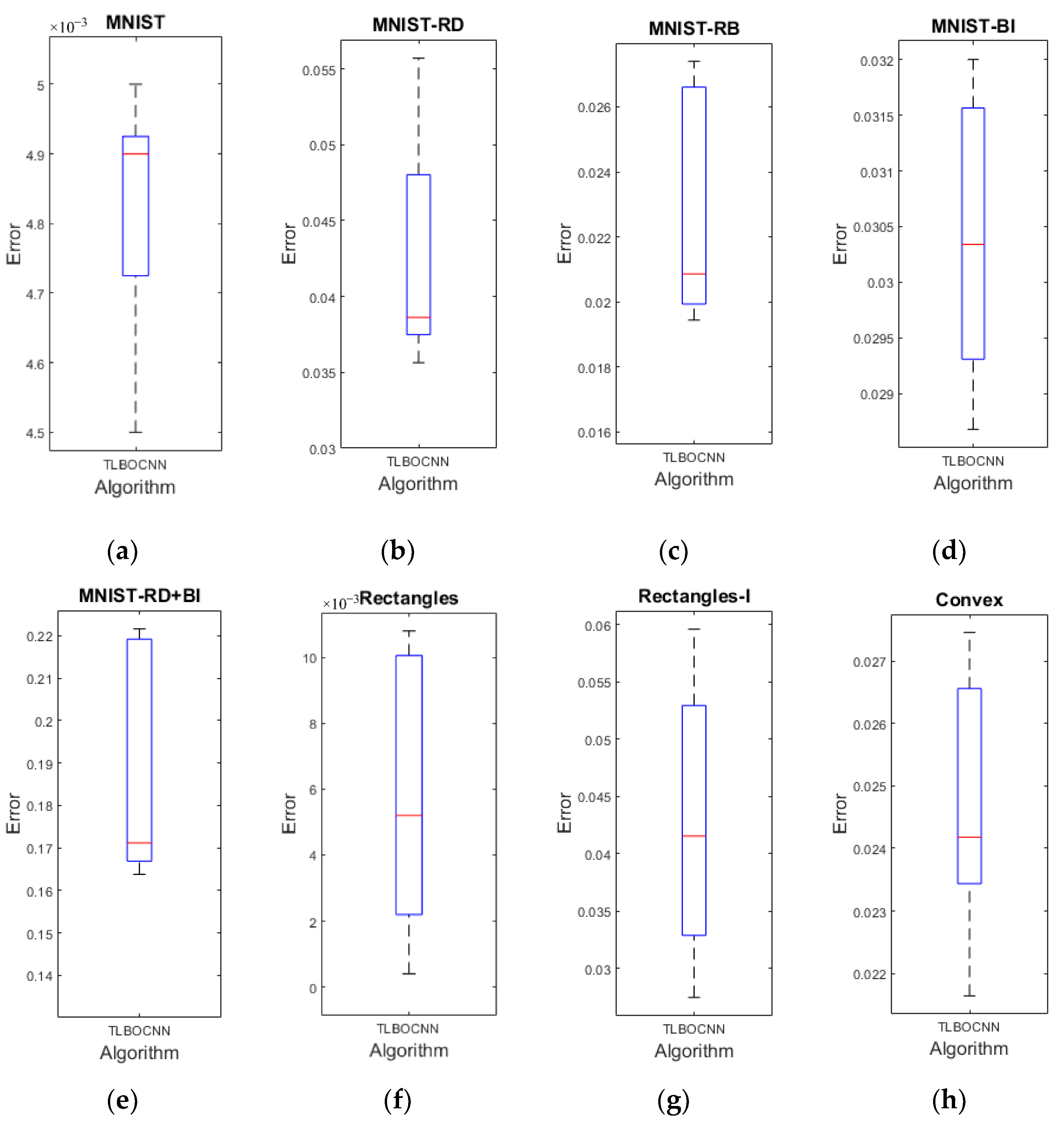
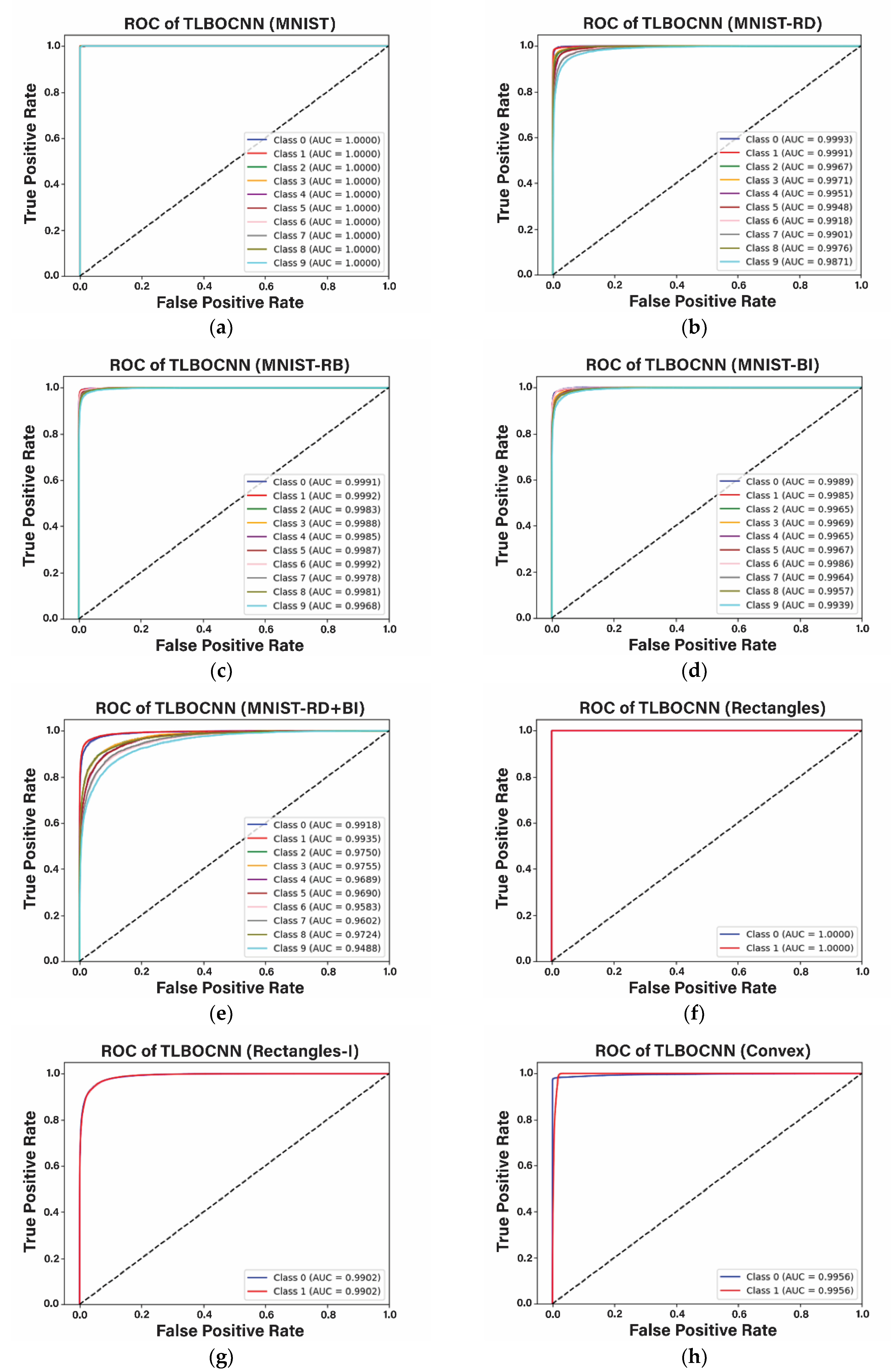
4.3.1. Performance Comparisons in Solving Eight Image Datasets

Table 4. Comparisons between TLBOCNN and its peers to solve the MNIST, MNIST-RD, MNIST-RB, MNIST-BI, MNIST-RD+BI, Rectangles, Rectangles-I, and Convex datasets.

Algorithms	MNIST	MNIST-RD	MNIST-RB	MNIST-BI	MNIST-RD+BI
RandNet-2	98.75% (+)	91.53% (+)	86.53% (+)	88.35% (+)	56.31% (+)
LDANet-2	98.95% (+)	92.48% (+)	93.19% (+)	87.58% (+)	61.46% (+)
CAE-1	98.60% (+)	95.48% (+)	93.19% (+)	87.58% (+)	61.46% (+)
CAE-2	97.52% (+)	90.34% (+)	89.10% (+)	84.50% (+)	54.77% (+)
ScatNet-2	98.73% (+)	92.52% (+)	87.70% (+)	81.60% (+)	49.52% (+)
SVM+RBF	96.97% (+)	88.89% (+)	85.42% (+)	77.49% (+)	44.82% (+)
SVM+Poly	96.31% (+)	84.58% (+)	83.38% (+)	75.99% (+)	43.59% (+)
PCANet-2	98.60% (+)	91.48% (+)	93.15% (+)	88.45% (+)	64.14% (+)
NNet	95.31% (+)	81.89% (+)	79.96% (+)	72.59% (+)	37.84% (+)
SAA-3	96.54% (+)	89.70% (+)	88.72% (+)	77.00% (+)	48.07% (+)
DBN-3	96.89% (+)	89.70% (+)	93.27% (+)	83.69% (+)	52.61% (+)
EvoCNN	98.82% (+)	94.78% (+)	97.20% (+)	95.47% (+)	64.97% (+)
psoCNN	99.51% (+)	94.56% (+)	97.61% (+)	96.87% (+)	81.05% (+)
TLBOCNN (Best)	99.55%	96.44%	98.06%	97.13%	83.64%
TLBOCNN (Mean)	99.52%	95.73%	97.72%	96.96%	81.14%
Algorithms	Rectangles	Rectangles-I	Convex	w/t/l	#BCA
RandNet-2	99.91% (+)	83.00% (+)	94.55% (+)	8/0/0	0
LDANet-2	99.86% (+)	83.80% (+)	92.78% (+)	8/0/0	0
CAE-1	99.86% (+)	83.80% (+)	NA	7/0/0	0
CAE-2	98.46% (+)	78.00% (+)	NA	7/0/0	0
ScatNet-2	99.99% (=)	91.98% (+)	93.50% (+)	7/1/0	0
SVM+RBF	97.85% (+)	75.96% (+)	80.87% (+)	8/0/0	0
SVM+Poly	97.85% (+)	75.95% (+)	80.18% (+)	8/0/0	0
PCANet-2	99.51% (+)	86.61% (+)	95.81% (+)	8/0/0	0
NNet	92.84% (+)	66.80% (+)	67.75% (+)	8/0/0	0
SAA-3	97.59% (+)	75.95% (+)	81.59% (+)	8/0/0	0
DBN-3	97.39% (+)	77.50% (+)	81.37% (+)	8/0/0	0
EvoCNN	99.99% (=)	94.97% (+)	95.18% (+)	7/1/0	1
psoCNN	99.93% (+)	96.03% (+)	97.74% (+)	8/0/0	0
TLBOCNN (Best)	99.99%	97.25%	97.84%	NA	8
TLBOCNN (Mean)	99.94%	95.72%	97.53%	NA	NA

presents the best classification accuracies produced by TLBOCNN and other peer algorithms in solving the eight image datasets, MNIST, MNIST-RD, MNIST-RB, MNIST-BI, MNIST-RD+BI, Rectangles, Rectangles-I, and Convex. Only the test sets of these eight image datasets are used to obtain the best classification accuracies of all algorithms for comparing their generalization capabilities. The compared algorithms that solve each image dataset with the best and second-best results are indicated with boldfaced and underlined fonts, respectively, as shown in Table 4. The signs of “(+)”, “(−)”, and “(=)” are also defined in Table 4 to indicate if the best classification accuracy produced by the proposed TLBOCNN in solving the test set of given image dataset is better than, worse than, or equal to those of its peer algorithms, respectively. Given that the results of most compared algorithms are extracted from the literature, “NA” in Table 4 implies that the results of compared algorithms to solve particular image datasets are unavailable. The performances of all compared algorithms in solving the eight selected image datasets are summarized as w/t/l and #BCA in Table 4. In particular, w/t/l implies that the optimal network architectures found by TLBOCNN outperform its peer algorithm in w datasets, ties with its peer algorithm in t datasets, and underperforms its peer algorithm in l datasets. Meanwhile, #BCA represents the number of best classification accuracy values produced by each compared algorithm to solve the eight selected image datasets.

Table 4 reports the proposed TLBOCNN as producing the best classification accuracies of 99.55%, 96.44%, 98.06%, 97.13%, 83.64%, 99.99%, 97.25%, and 97.84% when solving the MNIST, MNIST-RD, MNIST-RB, MNIST-BI, MNIST-RD+BI, Rectangles, Rectangles-I, and Convex datasets, respectively. The mean classification accuracies produced by TLBOCNN for these eight datasets are 99.52%, 95.73%, 97.72%, 96.96%, 81.14%, 99.94%, 95.72%, and 97.53%, respectively. From Table 4, the proposed TLBOCNN is best among all compared algorithms due to its excellent capability to solve the eight selected image datasets with the best accuracy. TLBOCNN is also observed to completely dominate RandNet-2. LDANet-2, CAE-1, CAE-2, SVM+RBF, SVM+Poly, PCANet-2, NNet, SAA-3, DBN-3, and psoCNN when solving these eight selected image datasets. Notably, the mean classification accuracies produced by TLBOCNN can outperform the other 13 peer algorithms when solving five out of eight image datasets (i.e., MNIST, MNIST-RD, MNIST-RB, MNIST-BI, and MNIST-RD+BI). For the Rectangles dataset, the proposed TLBOCNN, EvoCNN, and ScatNet-2 have produced the same best classification accuracy of 99.99%, followed by psoCNN, with a classification accuracy of 99.93%. Another interesting trend observed from Table 4 is that at least one of the metaheuristic-search-based methods (i.e., proposed TLBOCNN, EvoCNN, and psoCNN) has emerged as one of the top two performers in solving the eight selected image datasets. These observations have verified the promising potential of applying MSAs to automatically discover the optimal CNN network architectures and solve the given problems with promising performance without human intervention. Furthermore, the superior classification performances produced by the TLBOCNN compared to EvoCNN and psoCNN in solving the majority of image datasets also imply that the proposed method is incorporated with more robust search mechanisms that can achieve better balancing of exploration and exploitation strengths in searching for more appropriate CNN network architectures to solve the given datasets.

Apart from the quantitative analysis in Table 4, the performances of TLBOCNN in solving the eight selected datasets are also analyzed qualitatively. Figure 7 presents the boxplots indicating the distributions of test errors produced by TLBOCNN to solve these eight image datasets. TLBOCNN is proven to be able to consistently solve all image datasets with high classification accuracy. Another more balanced evaluation method used to analyze the effectiveness of optimal CNN architectures found by TLBOCNN is based on the receiver operating characteristic (ROC) curves and their corresponding area under curve (AUC) values, as shown in Figure 8. These AUC-ROC curves are constructed based on the true positive and false positive rates of TLBOCNN under different threshold settings when solving the eight selected image datasets. The values of AUC range from 0 to 1, where higher values imply better performance of the classifier. An ideal classifier has an AUC value of 1, whereas a classifier that makes random guesses has an AUC value of 0.5. Meanwhile, a classifier with AUC value of 0 tends to suffer with severe failure in the modelling process because it tends to predict a positive class as a negative class and vice versa. Referring to the locations of ROC curves and their corresponding AUCs that have values above 0.94, it is concluded that the optimal CNN network architectures found by TLBOCNN have good capabilities to distinguish one class from other classes for all selected image datasets.

To further analyze the performance difference among TLBOCNN and other peer algorithms in solving the eight selected image datasets, a set of non-parametric statistical analyses [83,84] was performed based on the results in Table 4. Both CAE-1 and CAE-2 are excluded due to the absence of their results for solving the Convex dataset. A Wilcoxon signed-rank test [84] is performed for pairwise comparison between TLBOCNN and other 11 peer algorithms to solve the eight image datasets. The pairwise comparison results of $R^{+}$, $R^{-}$, p-value, and h-value are reported in

Table 5. Wilcoxon signed-rank test results between TLBOCNN and its peer algorithms.

TLBOCNN (Best) vs.	${\mathit{R}}^{+}$	${\mathit{R}}^{-}$	p-Value	h-Value
RandNet-2	36.0	0.0	9.58 × 10−3	+
LDANet-2	36.0	0.0	9.58 × 10−3	+
ScatNet-2	28.0	0.0	1.42 × 10−2	+
SVM+RBF	36.0	0.0	9.58 × 10−3	+
SVM+Poly	36.0	0.0	9.58 × 10−3	+
PCANet-2	36.0	0.0	9.58 × 10−3	+
NNet	36.0	0.0	9.58 × 10−3	+
SAA-3	36.0	0.0	9.58 × 10−3	+
DBN-3	36.0	0.0	9.58 × 10−3	+
EvoCNN	28.0	0.0	1.23 × 10−2	+
psoCNN	36.0	0.0	5.34 × 10−3	+

. $R^{+}$ and $R^{-}$ are the sum of ranks at which TLBOCNN outperforms and underperforms each of its peers, respectively. The p-value is a minimum significance level used to detect differences between two algorithms. The algorithms with p-values smaller than a threshold value of $\alpha =0.05$ are significantly better than their compared methods. The h-value is obtained based on p andvalues to determine if TLBOCNN is significantly better (h = “+”), insignificant (h = “=”), or significantly worse (h = “−”) than its peer algorithms at solving all eight selected image datasets. From Table 5, it can be concluded that the proposed TLBOCNN is significantly better than all peer algorithms, as indicated by the h-values of “+” for all pairwise comparisons.

A Friedman test [83,84] is performed as a multiple comparisons analysis to evaluate the overall performance differences between TLBOCNN and the other 11 peer algorithms when solving the eight image datasets. From

Table 6. Average ranking and associated p-values produced through Friedman test.

Algorithms	Ranking	Chi-Square Statistic	p-Value
RandNet-2	6.0000	76.658654	0.00 × 10
LDANet-2	5.2500
ScatNet-2	5.8125
SVM+RBF	9.4375
SVM+Poly	10.5625
PCANet-2	5.2500
NNet	12.0000
SAA-3	9.0625
DBN-3	7.9375
EvoCNN	3.6250
psoCNN	2.5000
TLBOCNN (Best)	1.1250

, all compared algorithms are ranked by the Friedman test based on their classification accuracies from best to worst, as follows: TLBOCNN, psoCNN, EvoCNN, LDANet-2, PCANet-2, ScatNet-2, RandNet-2, DBN-3, SAA-3, SVM+RBF, SVM+Poly, and NNet. Table 6 also reveals that the p-value of Friedman test is lower than $\alpha =0.05$, implying significant global differences between all compared algorithms. Three post hoc statistical procedures [83] known as Bonferroni–Dunn, Holm, and Hochberg are then performed to further analyze the concrete differences by assigning TLBOCNN as a control algorithm. The results of z-values, unadjusted p-values, and adjusted p-values (APVs) are presented in

Table 7. Adjusted p-values of Bonferroni–Dunn, Holm, and Hochberg procedures.

TLBOCNN (Best) vs.	z	Unadjusted p	Bonferroni-Dunn p	Holm p	Hochberg p
NNet	6.03 × 10	0.00 × 10	0.00 × 10	0.00 × 10	0.00 × 10
SVM+Poly	5.23 × 10	0.00 × 10	2.00 × 10−6	2.00 × 10−6	2.00 × 10−6
SVM+RBF	4.61 × 10	4.00 × 10−6	4.40 × 10−5	3.60 × 10−5	3.60 × 10−5
SAA-3	4.40 × 10	1.10 × 10−5	1.17 × 10−4	8.50 × 10−5	8.50 × 10−5
DBN-3	3.78 × 10	1.58 × 10−4	1.73 × 10−3	1.10 × 10−3	1.10 × 10−3
RandNet-2	2.70 × 10	6.85 × 10−3	7.53 × 10−2	4.11 × 10−2	4.11 × 10−2
ScatNet-2	2.60 × 10	9.32 × 10−3	1.02 × 10−1	4.66 × 10−2	4.66 × 10−2
LDANet-2	2.29 × 10	2.21 × 10−2	2.43 × 10−1	8.85 × 10−2	6.64 × 10−2
PCANet-2	2.29 × 10	2.21 × 10−2	2.43 × 10−1	8.85 × 10−2	6.64 × 10−2
EvoCNN	1.07 × 10	2.82 × 10−1	3.11 × 10	5.65 × 10−1	4.46 × 10−1
psoCNN	7.63 × 10−1	4.46 × 10−1	4.90 × 10	5.65 × 10−1	4.45 × 10−1

. All post hoc procedures confirm the significant improvement of TLBOCNN over NNet, SVM+Poly, SVM+RBF, SAA-3, and DBN-3 because their APVs are smaller than $\alpha =0.05$. Holm and Hochberg procedures verify the significant improvements of TLBOCNN over RandNet02 and ScatNet-2.

4.3.2. Performance Comparisons in Solving Fashion Dataset

Table 8. Classification accuracies and number of parameters produced by the proposed TLBOCNN and other algorithms to solve Fashion dataset.

Algorithms	Classification Accuracy	# Parameters
Human Performance 1	83.50%	NA
2C1P2F+Dropout 1	91.60%	3.27 M
2C1P 1	92.50%	100 k
3C2F 1	90.70%	NA
3C1P2F+Dropout 1	92.60%	7.14 M
GRU+SVM 1	88.80%	NA
GRU+SVM+Dropout	89.70%	NA
HOG + SVM 1	92.60%	NA
ResNet-18 [25]	94.90%	11 M
VGG-16 [23]	93.50%	26 M
AlexNet [22]	89.90%	60 M
SqueezeNet-200 [82]	90.00%	500 k
MLP 256-128-64 1	90.00%	41 k
MLP 256-128-100 1	88.33%	3 M
EvoCNN [67]	94.53%	6.68 M
psoCNN [60]	92.81%	2.58 M
TLBOCNN (Best)	92.72%	414 k
TLBOCNN (Mean)	92.54%	1.56 M

¹https://github.com/zalandoresearch/fashion-mnist (accessed on 3 June 2022).

compares the performances of all algorithms in solving the Fashion dataset in terms of the classification accuracies and the network complexity represented by total numbers of parameters. Accordingly, ResNet-18, VGG-16, EvoCNN, psoCN, and TLBOCNN have emerged as the top five performers in solving the Fashion dataset, with classification accuracies of 94.90%, 93.50%, 94.53%, 92.81%, 92.72%, respectively. Similarly to Table 4, the simulation results in Table 8 also verify the benefits of using MSAs to automatically search for optimal CNN network architectures that can solve different classification problems competitively without requiring rich expert domain knowledge.

Although the classification accuracy produced by the proposed TLBOCNN for the Fashion dataset is slightly outperformed by those of ResNet-18, VGG-16, EvoCNN, and psoCNN, their performance differences are marginal, i.e., only 2.18%, 0.78%, 1.81%, and 0.09%, respectively. On the other hand, the best network architecture found by TLBOCNN to solve Fashion dataset only has 0.414 million parameters, and it is much less complicated that those of ResNet-18, VGG-16, EvoCNN, and psoCNN, which have total network parameter numbers of 11 million (i.e., 25.57 times higher), 26 million (i.e., 62.80 times higher), 6.68 million (i.e., 16.14 times higher), and 2.58 million (6.23 times highers), respectively. As compared to ResNet-18, VGG-16, EvoCNN, and psoCNN, the proposed TLBOCNN has exhibited better capability to achieve proper tradeoffs between classification accuracy and network complexity when designing optimal network architectures that can solve any given classification problems. In recent years, there has been growing demand for deploying deep learning algorithms in edge devices to solve various real-world applications, such as road condition monitoring systems, vehicle autopilot systems, and mobile devices. Most of these edge devices have limited computational power and battery capacity. Therefore, it is more desirable to deploy deep learning models that require lesser computing power and energy supply. The proposed TLBOCNN is envisioned as a potential solution for manufacturers given its promising capability to automatically search for less complex network architectures with good performances.

Other peer algorithms, such as AlexNet, 3C1P2F+Dropout, 2C1P2F+Dropout, and MLP 256-128-100, are observed to solve the Fashion dataset with worse accuracies than that of TLBOCNN despite the four former methods having more complex network architectures that consists of 60 million, 7.14 million, 3.27 million, and 3 million parameters, respectively. An important fact is revelated through these observations, i.e., most existing deep learning models designed with handcrafted approaches have excessive amounts of redundant parameters that tend to significantly increase the computational efforts without leading to any notable performance improvement in models in terms of classification accuracy. On the contrary, TLBOCNN can solve the Fashion dataset with competitive performance without requiring any data augmentation techniques nor complicated network architectures. Unlike most handcrafted deep learning networks that might feature feedback or parallel connections, the optimal network architectures found by TLBOCNN are simpler because the learners are initialized with smaller network architectures that can converge at a faster rate. The promising classification accuracy of TLBOCNN also implies the possibility of using smaller network architectures to achieve the state-of-the-art results.

4.3.3. Optimal Network Architecture Designed by TLBOCNN

The CNN network architectures designed by the proposed TLBOCNN to solve all nine selected image datasets with the highest classification accuracies are presented in

Table 9. Best CNN architecture produced by TLBOCNN for solving nine datasets.

Dataset	Layers	Parameters
MNIST	Convolutional	$numF=209$$,KS=4\times 4$
	Convolutional	$numF=170$$,KS=5\times 5$
	Convolutional	$numF=236$$,KS=6\times 6$
	Fully Connected	$numNeu=10$
MNIST-RD	Convolutional	$numF=71$$,KS=4\times 4$
	Convolutional	$numF=185$$,KS=6\times 6$
	Average Pooling	$\mathrm{Strides}=2\times 2$$,\mathrm{Pool}\mathrm{size}=3\times 3$
	Convolutional	$numF=215$$,KS=6\times 6$
	Fully Connected	$numNeu=10$
MNIST-RB	Convolutional	$numF=230$$,KS=3\times 3$
	Max Pooling	$\mathrm{Strides}=2\times 2$$,\mathrm{Pool}\mathrm{size}=3\times 3$
	Convolutional	$numF=195$$,KS=6\times 6$
	Convolutional	$numF=176$$,KS=4\times 4$
	Fully Connected	$numNeu=10$
MNIST-BI	Convolutional	$numF=173$$,KS=4\times 4$
	Convolutional	$numF=218$$,KS=4\times 4$
	Convolutional	$numF=183$$,KS=6\times 6$
	Convolutional	$numF=145$$,KS=6\times 6$
	Fully Connected	$numNeu=10$
MNIST-RD+BI	Convolutional	$numF=239$$,KS=4\times 4$
	Average Pooling	$\mathrm{Strides}=2\times 2$$,\mathrm{Pool}\mathrm{size}=3\times 3$
	Convolutional	$numF=160$$,KS=4\times 4$
	Convolutional	$numF=211$$,KS=6\times 6$
	Fully Connected	$numNeu=10$
Rectangles	Convolutional	$numF=208$$,KS=5\times 5$
	Average Pooling	$\mathrm{Strides}=2\times 2$$,\mathrm{Pool}\mathrm{size}=3\times 3$
	Convolutional	$numF=141$$,KS=5\times 5$
	Average Pooling	$\mathrm{Strides}=2\times 2$$,\mathrm{Pool}\mathrm{size}=3\times 3$
	Convolutional	$numF=176$$,KS=5\times 5$
	Fully Connected	$numNeu=2$
Rectangles-I	Convolutional	$numF=165$$,KS=4\times 4$
	Max Pooling	$\mathrm{Strides}=2\times 2$$,\mathrm{Pool}\mathrm{size}=3\times 3$
	Convolutional	$numF=236$$,KS=6\times 6$
	Convolutional	$numF=176$$,KS=5\times 5$
	Convolutional	$numF=176$$,KS=5\times 5$
	Fully Connected	$numNeu=2$
Convex	Convolutional	$numF=222$$,KS=4\times 4$
	Max Pooling	$\mathrm{Strides}=2\times 2$$,\mathrm{Pool}\mathrm{size}=3\times 3$
	Max Pooling	$\mathrm{Strides}=2\times 2$$,\mathrm{Pool}\mathrm{size}=3\times 3$
	Convolutional	$numF=229$$,KS=4\times 4$
	Convolutional	$numF=147$$,KS=5\times 5$
	Convolutional	$numF=191$$,KS=6\times 6$
	Fully Connected	$numNeu=2$
MNIST-Fashion	Convolutional	$numF=241$$,KS=5\times 5$
	Max Pooling	$\mathrm{Strides}=2\times 2$$,\mathrm{Pool}\mathrm{size}=3\times 3$
	Fully Connected	$numNeu=10$

. Accordingly, the optimal network architectures found by TLBOCNN to solve all image datasets only consist of one fully connected layer. This observation is consistent with recent findings in [85], i.e., a CNN network architecture with a single fully connected layer may produce better results than those with multiple fully connected layers. Table 9 also reveals that it is not always necessary to insert a pooling layer between two convolutional layers to solve certain image datasets (e.g., MNIST-RF, MNIST-RB, MNIST-BI, MNIST-RD+BI, Rectangle, and Convex) with the best classification accuracy. It is also possible to construct a CNN network architecture that can solve a dataset with the lowest error without incorporating any pooling layer, as shown in MNIST and MNIST-BI. In other words, the search mechanisms incorporated into the proposed TLBOCNN can prevent the inclusion of any redundant layers or parameters into network architectures if they are unable to offer any meaningful network performance gains. This desirable characteristic has justified the excellent capability of the proposed TLBOCNN to automatically discover the optimal network architectures that can solve the given classification tasks without requiring any domain knowledge of the problems.

5. Conclusions

A new network architecture design method known as TLBOCNN is proposed to automatically search for optimal CNN network architectures that can solve different classification problems effectively and efficiently without requiring rich expert domain knowledge. The hyperparameters of CNN networks optimized by TLBOCNN include the number of layers, type of layers, kernel sizes, number of filters, and umber of neurons. To achieve this goal, an appropriate solution-encoding strategy is introduced into TLBOCNN to facilitate the representation of CNN network architectures with flexible sizes by learners with variable length. Design constraints are also introduced to prevent the construction of invalid network architectures without compromising the ability of TLBOCN to search for novel network architectures. During the teacher phase of TLBOCNN, a novel mainstream architecture computation scheme is designed to determine population mean by referring to all learners with different lengths. A new difference operator is also introduced in both the teacher and learner phases of TLBOCNN to compare the differences between two learners with variable length followed by the design of a new position update operator used to search for the new CNN models that are represented by updated TLBO learners. The proposed TLBOCNN is compared to various state-of-the-art deep learning algorithms using nine different image datasets. Extensive simulation studies reveal that TLBOCNN can perform significantly better than most peer algorithms by solving the selected image datasets with higher classification accuracies. TLBOCNN is also able to search for optimal network architectures that can achieve proper tradeoffs between classification accuracy and network complexity when solving the given problems.

Despite the promising performances exhibited by TLBOCNN, some of its limitations are explained as follows. First, the current version of TLBOCNN only considers three types of functional blocks (i.e., convolutional, pooling and fully connected layers) when searching for the optimal network architectures of CNN. The potentials of other more sophisticated building blocks (e.g., ResNet, DenseNet, Inception, NASNet, etc.) to further enhance network performance are yet to be investigated by TLBOCNN. Some recent studies conducted in [68] revealed the feasibility of considering both ResNet and DenseNet blocks when designing the CNN network architectures without having to make substantial modifications to the original search operators of MSAs. Second, the search operators of TLBOCNN are similar to those of the original TLBO except for the modifications made to handle the variable-length learners issue. The original TLBO tends to suffer from the premature convergence issue when solving complex problems because its search operators rely on historical information (i.e., teacher solution and population mean), which is less frequently updated in the latter optimization stage. Similar challenges might be encountered by TLBOCNN when solving more complex real-world classification problems. Third, the network design method considered in the current study is a single optimization problem in which classification accuracy is the only criterion used to evaluate the quality of network architectures represented by each TLBOCNN. In practical scenarios, manufacturers must consider multiple criteria when selecting suitable network architectures for their applications. It is more desirable have a network design method that can generate multiple network architectures so that the manufacturers can make better decisions based on their current needs. Referring to these limitations, some future works can be proposed as extensions of the current work. First, the proposed TLBOCNN can be further enhanced by considering other sophisticated building blocks, such as ResNet block, DenseNet block, Inception block, NASNet block, etc., when it is used to design optimal CNN network architectures for solving given classification problems. Second, further modifications can be introduced to the search operators of TLBOCNN to achieve better balancing of exploration and exploitation searches, hence reducing its likelihood of suffering from premature convergence and enhancing its ability to search for more promising network architectures when solving more complex real-world classification problems. Finally, it is also worth investigating the possibility of formulating network architecture design as a multi-objective optimization problem in which different contradictory requirements, such as classification accuracy, network complexity, inference speed, etc., can be taken into account during the optimization process to produce multiple CNN network architectures with different characteristics.

References

1. Carvalho, M.; Ludermir, T.B. Particle swarm optimization of neural network architectures andweights. In Proceedings of the 7th International Conference on Hybrid Intelligent Systems (HIS 2007), Kaiserslautern, Germany, 17–19 September 2007; pp. 336–339. [Google Scholar]
2. Sainath, T.N.; Mohamed, A.-R.; Kingsbury, B.; Ramabhadran, B. Deep convolutional neural networks for LVCSR. In Proceedings of the 2013 IEEE international Conference on Acoustics, Speech and Signal Processing, Vancouver, BC, Canada, 26–31 May 2013; pp. 8614–8618. [Google Scholar]
3. Syulistyo, A.R.; Purnomo, D.M.J.; Rachmadi, M.F.; Wibowo, A. Particle swarm optimization (PSO) for training optimization on convolutional neural network (CNN). J. Ilmu Komput. Dan Inf. 2016, 9, 52–58. [Google Scholar] [CrossRef]
4. Rodriguez, P.; Wiles, J.; Elman, J.L. A recurrent neural network that learns to count. Connect. Sci. 1999, 11, 5–40. [Google Scholar] [CrossRef] [Green Version]
5. Sumachev, A.E.; Kuzmin, V.A.; Borodin, E.S. River flow forecasting using artificial neural networks. Int. J. Mech. Eng. Technol. 2018, 9, 706–714. [Google Scholar]
6. Hu, M.; Wu, Y.; Fan, J.; Jing, B. Joint Semantic Intelligent Detection of Vehicle Color under Rainy Conditions. Mathematics 2022, 10, 3512. [Google Scholar] [CrossRef]
7. Alotaibi, M.F.; Omri, M.; Abdel-Khalek, S.; Khalil, E.; Mansour, R.F. Computational Intelligence-Based Harmony Search Algorithm for Real-Time Object Detection and Tracking in Video Surveillance Systems. Mathematics 2022, 10, 733. [Google Scholar] [CrossRef]
8. Maturana, D.; Scherer, S. Voxnet: A 3d convolutional neural network for real-time object recognition. In Proceedings of the 2015 IEEE/RSJ International Conference on Intelligent Robots and Systems (IROS), Hamburg, Germany, 28 September–3 October 2015; p. 922. [Google Scholar]
9. Abdelhamid, A.A.; El-Kenawy, E.-S.M.; Alotaibi, B.; Amer, G.M.; Abdelkader, M.Y.; Ibrahim, A.; Eid, M.M. Robust Speech Emotion Recognition Using CNN+ LSTM Based on Stochastic Fractal Search Optimization Algorithm. IEEE Access 2022, 10, 49265–49284. [Google Scholar] [CrossRef]
10. Fan, C.-L.; Chung, Y.-J. Design and Optimization of CNN Architecture to Identify the Types of Damage Imagery. Mathematics 2022, 10, 3483. [Google Scholar] [CrossRef]
11. Feng, X.; Gao, X.; Luo, L. A ResNet50-Based Method for Classifying Surface Defects in Hot-Rolled Strip Steel. Mathematics 2021, 9, 2359. [Google Scholar] [CrossRef]
12. Khurma, R.A.; Alsawalqah, H.; Aljarah, I.; Elaziz, M.A.; Damaševičius, R. An Enhanced Evolutionary Software Defect Prediction Method Using Island Moth Flame Optimization. Mathematics 2021, 9, 1722. [Google Scholar] [CrossRef]
13. Boikov, A.; Payor, V.; Savelev, R.; Kolesnikov, A. Synthetic data generation for steel defect detection and classification using deep learning. Symmetry 2021, 13, 1176. [Google Scholar] [CrossRef]
14. Deng, H.; Cheng, Y.; Feng, Y.; Xiang, J. Industrial Laser Welding Defect Detection and Image Defect Recognition Based on Deep Learning Model Developed. Symmetry 2021, 13, 1731. [Google Scholar] [CrossRef]
15. El-kenawy, E.-S.M.; Albalawi, F.; Ward, S.A.; Ghoneim, S.S.; Eid, M.M.; Abdelhamid, A.A.; Bailek, N.; Ibrahim, A. Feature selection and classification of transformer faults based on novel meta-heuristic algorithm. Mathematics 2022, 10, 3144. [Google Scholar] [CrossRef]
16. Alhussan, A.A.; Khafaga, D.S.; El-Kenawy, E.-S.M.; Ibrahim, A.; Eid, M.M.; Abdelhamid, A.A. Pothole and Plain Road Classification Using Adaptive Mutation Dipper Throated Optimization and Transfer Learning for Self Driving Cars. IEEE Access 2022, 10, 84188–84211. [Google Scholar] [CrossRef]
17. Xin, R.; Zhang, J.; Shao, Y. Complex network classification with convolutional neural network. Tsinghua Sci. Technol. 2020, 25, 447–457. [Google Scholar] [CrossRef]
18. Acharya, U.R.; Oh, S.L.; Hagiwara, Y.; Tan, J.H.; Adam, M.; Gertych, A.; San Tan, R. A deep convolutional neural network model to classify heartbeats. Comput. Biol. Med. 2017, 89, 389–396. [Google Scholar] [CrossRef]
19. Khafaga, D.S.; Alhussan, A.A.; El-Kenawy, E.-S.M.; Ibrahim, A.; Eid, M.M.; Abdelhamid, A.A. Solving Optimization Problems of Metamaterial and Double T-Shape Antennas Using Advanced Meta-Heuristics Algorithms. IEEE Access 2022, 10, 74449–74471. [Google Scholar] [CrossRef]
20. He, K.; Zhang, X.; Ren, S.; Sun, J. Delving deep into rectifiers: Surpassing human-level performance on imagenet classification. In Proceedings of the IEEE International Conference on Computer Vision, Santiago, Chile, 7–13 December 2015; pp. 1026–1034. [Google Scholar]
21. Szegedy, C.; Liu, W.; Jia, Y.; Sermanet, P.; Reed, S.; Anguelov, D.; Erhan, D.; Vanhoucke, V.; Rabinovich, A. Going deeper with convolutions. In Proceedings of the IEEE Conference On Computer Vision and Pattern Recognition, Santiago, Chile, 7–13 December 2015; pp. 1–9. [Google Scholar]
22. Krizhevsky, A.; Sutskever, I.; Hinton, G.E. Imagenet classification with deep convolutional neural networks. Commun. ACM 2017, 60, 84–90. [Google Scholar] [CrossRef] [Green Version]
23. Simonyan, K.; Zisserman, A. Very deep convolutional networks for large-scale image recognition. arXiv 2014, arXiv:1409.1556. [Google Scholar] [CrossRef]
24. Huang, G.; Liu, Z.; Van Der Maaten, L.; Weinberger, K.Q. Densely connected convolutional networks. In Proceedings of the IEEE Conference on Computer Vision and Pattern Recognition, Honolulu, HI, USA, 21–26 July 2017; pp. 4700–4708. [Google Scholar]
25. He, K.; Zhang, X.; Ren, S.; Sun, J. Deep residual learning for image recognition. In Proceedings of the IEEE Conference on Computer Vision and Pattern Recognition, Las Vegas, NV, USA, 27–30 June 2016; pp. 770–778. [Google Scholar]
26. Bergstra, J.; Bengio, Y. Random search for hyper-parameter optimization. J. Mach. Learn. Res. 2012, 13, 281–305. [Google Scholar]
27. Kaelbling, L.P.; Littman, M.L.; Moore, A.W. Reinforcement learning: A survey. J. Artif. Intell. Res. 1996, 4, 237–285. [Google Scholar] [CrossRef] [Green Version]
28. Liu, H.; Simonyan, K.; Yang, Y. Darts: Differentiable architecture search. arXiv 2018, arXiv:1806.09055. [Google Scholar] [CrossRef]
29. Bäck, T.; Fogel, D.B.; Michalewicz, Z. Handbook of evolutionary computation. Release 1997, 97, B1. [Google Scholar] [CrossRef]
30. Baker, B.; Gupta, O.; Naik, N.; Raskar, R. Designing neural network architectures using reinforcement learning. arXiv 2016, arXiv:1611.02167. [Google Scholar] [CrossRef]
31. Zoph, B.; Le, Q.V. Neural architecture search with reinforcement learning. arXiv 2016, arXiv:1611.01578. [Google Scholar] [CrossRef]
32. Melanie, M. An Introduction to Genetic Algorithms; Massachusetts Institute of Technology: Cambridge, MA, USA, 1996; p. 158. [Google Scholar]
33. Kennedy, J.; Eberhart, R. Particle swarm optimization. In Proceedings of the ICNN’95—International Conference on Neural Networks, Perth, WA, Australia, 27 November–1 December 1995; Volume 1944, pp. 1942–1948. [Google Scholar]
34. Storn, R.; Price, K. Differential Evolution—A Simple and Efficient Heuristic for global Optimization over Continuous Spaces. J. Glob. Optim. 1997, 11, 19. [Google Scholar] [CrossRef]
35. Rao, R.V.; Savsani, V.J.; Vakharia, D.P. Teaching–learning-based optimization: A novel method for constrained mechanical design optimization problems. Comput.-Aided Des. 2011, 43, 303–315. [Google Scholar] [CrossRef]
36. Behera, M.; Sarangi, A.; Mishra, D.; Mallick, P.K.; Shafi, J.; Srinivasu, P.N.; Ijaz, M.F. Automatic Data Clustering by Hybrid Enhanced Firefly and Particle Swarm Optimization Algorithms. Mathematics 2022, 10, 3532. [Google Scholar] [CrossRef]
37. Chen, J.; Chen, M.; Wen, J.; He, L.; Liu, X. A Heuristic Construction Neural Network Method for the Time-Dependent Agile Earth Observation Satellite Scheduling Problem. Mathematics 2022, 10, 3498. [Google Scholar] [CrossRef]
38. Qiu, J.; Yin, X.; Pan, Y.; Wang, X.; Zhang, M. Prediction of Uniaxial Compressive Strength in Rocks Based on Extreme Learning Machine Improved with Metaheuristic Algorithm. Mathematics 2022, 10, 3490. [Google Scholar] [CrossRef]
39. Kaya, E. A New Neural Network Training Algorithm Based on Artificial Bee Colony Algorithm for Nonlinear System Identification. Mathematics 2022, 10, 3487. [Google Scholar] [CrossRef]
40. Ma, Z.; Yuan, X.; Han, S.; Sun, D.; Ma, Y. Improved chaotic particle swarm optimization algorithm with more symmetric distribution for numerical function optimization. Symmetry 2019, 11, 876. [Google Scholar] [CrossRef] [Green Version]
41. Zhang, M.; Long, D.; Qin, T.; Yang, J. A chaotic hybrid butterfly optimization algorithm with particle swarm optimization for high-dimensional optimization problems. Symmetry 2020, 12, 1800. [Google Scholar] [CrossRef]
42. El-Kenawy, E.-S.M.; Mirjalili, S.; Alassery, F.; Zhang, Y.-D.; Eid, M.M.; El-Mashad, S.Y.; Aloyaydi, B.A.; Ibrahim, A.; Abdelhamid, A.A. Novel Meta-Heuristic Algorithm for Feature Selection, Unconstrained Functions and Engineering Problems. IEEE Access 2022, 10, 40536–40555. [Google Scholar] [CrossRef]
43. El-Kenawy, E.-S.M.; Mirjalili, S.; Abdelhamid, A.A.; Ibrahim, A.; Khodadadi, N.; Eid, M.M. Meta-heuristic optimization and keystroke dynamics for authentication of smartphone users. Mathematics 2022, 10, 2912. [Google Scholar] [CrossRef]
44. Liu, X.-J.; Yi, H.; Ni, Z.-H. Application of ant colony optimization algorithm in process planning optimization. J. Intell. Manuf. 2013, 24, 1–13. [Google Scholar] [CrossRef]
45. Meng, A.-B.; Chen, Y.-C.; Yin, H.; Chen, S.-Z. Crisscross optimization algorithm and its application. Knowl.-Based Syst. 2014, 67, 218–229. [Google Scholar] [CrossRef]
46. Gharehchopogh, F.S.; Maleki, I.; Dizaji, Z.A. Chaotic vortex search algorithm: Metaheuristic algorithm for feature selection. Evol. Intell. 2022, 15, 1777–1808. [Google Scholar] [CrossRef]
47. Ahmad, M.F.; Isa, N.A.M.; Lim, W.H.; Ang, K.M. Differential evolution: A recent review based on state-of-the-art works. Alex. Eng. J. 2022, 61, 3831–3872. [Google Scholar] [CrossRef]
48. LeCun, Y.; Bengio, Y. Convolutional networks for images, speech, and time series. In The Handbook of Brain Theory and Neural Networks; MIT Press: Cambridge, MA, USA, 1998. [Google Scholar]
49. Schaffer, J.D.; Caruana, R.A.; Eshelman, L.J. Using genetic search to exploit the emergent behavior of neural networks. Phys. D Nonlinear Phenom. 1990, 42, 244–248. [Google Scholar] [CrossRef]
50. Kitano, H. Empirical studies on the speed of convergence of neural network training using genetic algorithms. In Proceedings of the AAAI Conference on Artificial Intelligence-1990, Boston, MA, USA, 29 July–3 August 1990; pp. 789–795. [Google Scholar]
51. Stanley, K.O.; Miikkulainen, R. Evolving neural networks through augmenting topologies. Evol. Comput. 2002, 10, 99–127. [Google Scholar] [CrossRef]
52. Siebel, N.T.; Sommer, G. Evolutionary reinforcement learning of artificial neural networks. Int. J. Hybrid Intell. Syst. 2007, 4, 171–183. [Google Scholar] [CrossRef] [Green Version]
53. Stanley, K.O.; D’Ambrosio, D.B.; Gauci, J. A hypercube-based encoding for evolving large-scale neural networks. Artif. Life 2009, 15, 185–212. [Google Scholar] [CrossRef] [PubMed]
54. Verbancsics, P.; Harguess, J. Generative neuroevolution for deep learning. arXiv 2013, arXiv:1312.5355. [Google Scholar] [CrossRef]
55. LeCun, Y.; Bottou, L.; Bengio, Y.; Haffner, P. Gradient-based learning applied to document recognition. Proc. IEEE 1998, 86, 2278–2324. [Google Scholar] [CrossRef] [Green Version]
56. Albeahdili, H.M.; Han, T.; Islam, N.E. Hybrid algorithm for the optimization of training convolutional neural network. Int. J. Adv. Comput. Sci. Appl. 2015, 1, 79–85. [Google Scholar]
57. Krizhevsky, A.; Hinton, G. Learning Multiple Layers of Features from Tiny Images; Technical Report; University of Toronto: Toronto, ON, Canada, 2009; Available online: http://www.cs.utoronto.ca/~kriz/learning-features-2009-TR.pdf (accessed on 3 June 2022).
58. Sermanet, P.; Chintala, S.; LeCun, Y. Convolutional neural networks applied to house numbers digit classification. In Proceedings of the 21st International Conference on Pattern Recognition (ICPR2012), Tsukuba, Japan, 11–15 November 2012; pp. 3288–3291. [Google Scholar]
59. Wang, B.; Sun, Y.; Xue, B.; Zhang, M. Evolving deep convolutional neural networks by variable-length particle swarm optimization for image classification. In Proceedings of the 2018 IEEE Congress on Evolutionary Computation (CEC), Rio de Janeiro, Brazil, 8–13 July 2018; pp. 1–8. [Google Scholar]
60. Junior, F.E.F.; Yen, G.G. Particle swarm optimization of deep neural networks architectures for image classification. Swarm Evol. Comput. 2019, 49, 62–74. [Google Scholar] [CrossRef]
61. Sun, Y.; Xue, B.; Zhang, M.; Yen, G.G. A particle swarm optimization-based flexible convolutional autoencoder for image classification. IEEE Trans. Neural Netw. Learn. Syst. 2018, 30, 2295–2309. [Google Scholar] [CrossRef] [Green Version]
62. Koza, J.R. Genetic Programming; MIT Press: Cambridge, MA, USA, 1997. [Google Scholar]
63. Oullette, R.; Browne, M.; Hirasawa, K. Genetic algorithm optimization of a convolutional neural network for autonomous crack detection. In Proceedings of the 2004 Congress on Evolutionary Computation (IEEE Cat. No. 04TH8753), Portland, OR, USA, 19–23 June 2004; pp. 516–521. [Google Scholar]
64. Ijjina, E.P.; Chalavadi, K.M. Human action recognition using genetic algorithms and convolutional neural networks. Pattern Recognit. 2016, 59, 199–212. [Google Scholar] [CrossRef]
65. Reddy, K.K.; Shah, M. Recognizing 50 human action categories of web videos. Mach. Vis. Appl. 2013, 24, 971–981. [Google Scholar] [CrossRef] [Green Version]
66. Young, S.R.; Rose, D.C.; Karnowski, T.P.; Lim, S.-H.; Patton, R.M. Optimizing deep learning hyper-parameters through an evolutionary algorithm. In Proceedings of the Workshop on Machine Learning in High-Performance Computing Environments, Austin, TX, USA, 15 November 2015; pp. 1–5. [Google Scholar]
67. Sun, Y.; Xue, B.; Zhang, M.; Yen, G.G. Evolving deep convolutional neural networks for image classification. IEEE Trans. Evol. Comput. 2019, 24, 394–407. [Google Scholar] [CrossRef] [Green Version]
68. Xue, Y.; Wang, Y.; Liang, J.; Slowik, A. A self-adaptive mutation neural architecture search algorithm based on blocks. IEEE Comput. Intell. Mag. 2021, 16, 67–78. [Google Scholar] [CrossRef]
69. Suganuma, M.; Shirakawa, S.; Nagao, T. A genetic programming approach to designing convolutional neural network architectures. In Proceedings of the Genetic and Evolutionary Computation Conference, Berlin, Germany, 15–19 July 2017; pp. 497–504. [Google Scholar]
70. Harding, S. Evolution of image filters on graphics processor units using cartesian genetic programming. In Proceedings of the 2008 IEEE Congress on Evolutionary Computation (IEEE World Congress on Computational Intelligence), Hong Kong, China, 1–6 June 2008; pp. 1921–1928. [Google Scholar]
71. Miller, J.F.; Smith, S.L. Redundancy and computational efficiency in cartesian genetic programming. IEEE Trans. Evol. Comput. 2006, 10, 167–174. [Google Scholar] [CrossRef]
72. Miller, J.F.; Harding, S.L. Cartesian genetic programming. In Proceedings of the 11th Annual Conference Companion on Genetic and Evolutionary Computation Conference: Late Breaking Papers, Montreal, QC, Canada, 8–12 July 2009; pp. 3489–3512. [Google Scholar]
73. Wang, B.; Sun, Y.; Xue, B.; Zhang, M. A hybrid differential evolution approach to designing deep convolutional neural networks for image classification. In Proceedings of the Australasian Joint Conference on Artificial Intelligence, Wellington, New Zealand, 11–14 December 2018; pp. 237–250. [Google Scholar]
74. Dahou, A.; Elaziz, M.A.; Zhou, J.; Xiong, S. Arabic sentiment classification using convolutional neural network and differential evolution algorithm. Comput. Intell. Neurosci. 2019, 2019, 2537689. [Google Scholar] [CrossRef] [PubMed]
75. Ghosh, A.; Jana, N.D.; Mallik, S.; Zhao, Z. Designing optimal convolutional neural network architecture using differential evolution algorithm. Patterns 2022, 3, 100567. [Google Scholar] [CrossRef]
76. Kingma, D.P.; Ba, J. Adam: A method for stochastic optimization. arXiv 2014, arXiv:1412.6980. [Google Scholar]
77. Larochelle, H.; Erhan, D.; Courville, A.; Bergstra, J.; Bengio, Y. An empirical evaluation of deep architectures on problems with many factors of variation. In Proceedings of the 24th International Conference on Machine Learning, Virtual, 13–15 April 2021; pp. 473–480. [Google Scholar]
78. Xiao, H.; Rasul, K.; Vollgraf, R. Fashion-mnist: A novel image dataset for benchmarking machine learning algorithms. arXiv 2017, arXiv:1708.07747. [Google Scholar]
79. Chan, T.-H.; Jia, K.; Gao, S.; Lu, J.; Zeng, Z.; Ma, Y. PCANet: A simple deep learning baseline for image classification? IEEE Trans. Image Process. 2015, 24, 5017–5032. [Google Scholar] [CrossRef] [Green Version]
80. Rifai, S.; Vincent, P.; Muller, X.; Glorot, X.; Bengio, Y. Contractive auto-encoders: Explicit invariance during feature extraction. In Proceedings of ICML’11 Proceedings of the 28th International Conference on International Conference on Machine Learning, Bellevue, WA, USA, 28 June–2 July 2011. [Google Scholar]
81. Bruna, J.; Mallat, S. Invariant scattering convolution networks. IEEE Trans. Pattern Anal. Mach. 2013, 35, 1872–1886. [Google Scholar] [CrossRef] [Green Version]
82. Iandola, F.N.; Han, S.; Moskewicz, M.W.; Ashraf, K.; Dally, W.J.; Keutzer, K. SqueezeNet: AlexNet-level accuracy with 50x fewer parameters and <0.5 MB model size. arXiv 2016, arXiv:1602.07360. [Google Scholar]
83. Derrac, J.; García, S.; Molina, D.; Herrera, F. A practical tutorial on the use of nonparametric statistical tests as a methodology for comparing evolutionary and swarm intelligence algorithms. Swarm Evol. Comput. 2011, 1, 3–18. [Google Scholar] [CrossRef]
84. García, S.; Molina, D.; Lozano, M.; Herrera, F. A study on the use of non-parametric tests for analyzing the evolutionary algorithms’ behaviour: A case study on the CEC’2005 special session on real parameter optimization. J. Heuristics 2009, 15, 617–644. [Google Scholar] [CrossRef]
85. Springenberg, J.T.; Dosovitskiy, A.; Brox, T.; Riedmiller, M. Striving for simplicity: The all convolutional net. arXiv 2014, arXiv:1412.6806. [Google Scholar]
Figure 1. Typical network architecture of a sequential CNN.
Symmetry 14 02323 g001
Figure 2. Representation of a potential CNN network architecture by a TLBOCNN learner.
Symmetry 14 02323 g002
Figure 3. Mechanisms used to construct mainstream CNN architecture of TLBOCNN with N = 5.
Symmetry 14 02323 g003
Figure 4. Graphical illustration of mechanisms used to calculate the differences between two learners, L1 and L2, that represent CNN models with different network architectures.
Symmetry 14 02323 g004
Figure 5. Mechanisms used to calculate X n n e w . B l o c k s based on L D i f f and X n . B l o c k s .
Symmetry 14 02323 g005
Figure 6. Sample images from the image datasets of (a) MNIST, (b) MNIST-RD, (c) MNIST-RB, (d) MNIST-BI, (e) MNIST-RD+BI, (f) Rectangles, (g) Rectangles-I, (h) Convex, and (i) Fashion.
Symmetry 14 02323 g006
Figure 7. Test errors produced by TLBOCNN while solving (a) MNIST, (b) MNIST-RD, (c) MNIST-RB, (d) MNIST-BI, (e) MNIST-RD+BI, (f) Rectangles, (g) Rectangles-I, and (h) Convex datasets.
Symmetry 14 02323 g007
Figure 8. AUR-ROC curves of TLBOCNN while solving (a) MNIST, (b) MNIST-RD, (c) MNIST-RB, (d) MNIST-BI, (e) MNIST-RD+BI, (f) Rectangles, (g) Rectangles-I, and (h) Convex datasets. The dotted line is a baseline method to indicate a classifier with random prediction capability.
Symmetry 14 02323 g008