Article

MHD Pulsatile Flow of Blood-Based Silver and Gold Nanoparticles between Two Concentric Cylinders

by
Faisal Shahzad
1,
Wasim Jamshed
1,*,
Farheen Aslam
2,
Rasheeda Bashir
2,
El Sayed M. Tag El Din
3,
Hamiden Abd El-Wahed Khalifa
4,5 and
Agaeb Mahal Alanzi
5
1
Department of Mathematics, Capital University of Science and Technology (CUST), Islamabad 44000, Pakistan
2
Department of Biotechnology, Lahore College for Women University, Lahore 54000, Pakistan
3
Electrical Engineering, Faculty of Engineering and Technology, Future University in Egypt, New Cairo 11835, Egypt
4
Department of Operations Research, Faculty of Graduate Studies for Statistical Research, Cairo University, Giza 12613, Egypt
5
Department of Mathematics, College of Science and Arts, Qassim University, Al-Badaya 51951, Saudi Arabia
*
Author to whom correspondence should be addressed.
Symmetry 2022, 14(11), 2254; https://doi.org/10.3390/sym14112254
Submission received: 6 September 2022 / Revised: 20 October 2022 / Accepted: 21 October 2022 / Published: 27 October 2022
(This article belongs to the Special Issue Symmetry of Nanofluids and Their Applications in Engineering)

Abstract

:
Pulsatory movements appear in a variety of fascinating applications involving periodic flow propagation and control. Pulsing encourages mixing and, as a result, mass and heat exchange with the boundaries. Pulsing also helps to decrease surface fouling by allowing solid particles to migrate. An exact solution of the Navier–Stokes equations for the transport of an incompressible viscous fluid in a channel with arbitrary pressure distribution is described in this study. The flow is defined by two primary parameters: the pulsation parameter, which is determined by the periodic pressure gradient, and the kinetic Reynolds number, which is determined by the pulsation frequency. The purpose of employing hybrid nanofluid (HNF) is to increase the base fluid’s thermal conductivity. We regard Ag and Au as nanoparticles (NPs) and blood as a base fluid for this phenomenon. Broadening this reveals that the consideration of nanoparticles has impressively extended the warm movement at the parcels of both turbulent and laminar frameworks. Attention is paid to the slope of speed, temperature, and voltage. The geometric model is therefore described using a symmetry technique. We developed the governing equation for this problem’s analytical solutions. The velocity and temperature fields solution is given in the form of the Bessel and modified Bessel functions. Graph results show the mathematical benefits of the current limits: for instance, Hartmann number M , solid volume part of nanoparticles ϕ , Reynolds number R e β , Prandtl number P r , intermittent slob limit, etc. The strain angles introduced in the stress contrast, frictional force, velocity profile, and temperature profile were obtained, and the characteristics of the vortex were investigated. Resources at various boundaries of the perceptual flow are examined. As with the final essence, the smoothest results are analyzed and recorded. It has also been discovered that the velocity may be regulated by the external magnetic field, which affects the temperature profiles and hence the heat transfer, which can be enhanced or lowered by mastering the magnetic field.

1. Introduction

Pulsating floating work has sparked substantial attention, owing principally to several commercial-level experiments. The pulsing flow of waves transmitted along the duct wall determines the flowing in the duct/cylinder, which is produced in a roughly sinusoidal form. There are fundamentally some significant packages when it comes to the fluids that monitor vibrating floats. In clinical science, relevant concepts include blood flow via courses, peristaltic formation of food in the digestive system, and urine stream in the urethra. Moreover, in astronomy and geophysics, research concentrates on heavenly shapes, ground centers, and sun-powered plasmas [1]. Vardanyan et al. [2] have created numerous hypothetical models for the outcomes of the attractive energy of throbbing streams. You said that if the energy of the magnet is regular and stable, the magnetic flux charge will decrease. Her work had a great influence on organic research. Richardson and Tyler [3,4] have shown exploratory outcomes on the presence of oscillating currents, or organisms that contribute to the so-called ring impact. Ensuing examinations by Womersley [5] and Uchida [6] summed up these outcomes by concentrating on the sinusoidal movements answerable for incompressible wavering liquids along level conductors. Aside from all the hypothetical studies above, current international programs deal with different body shapes in the context of existing evaluations, as shown with the help of different authors. Recently, Yang et al. [7] incorporated the optimization of a complete cylinder with a pin fin heatsink using the finite quantity method (FVM). Most thermal switch loads are applied because their goal is to maintain the total amount of heatsink and fin material while performing load damping to assess the overall hydraulic performance of the system. In a study by Cui et al. [8], they have defined parametric representations for estimating overall thermal performance. It deals with the random heat exchange of modern countercurrent evaporation. It turns out that this phenomenon expects the overall performance of the countercurrent playback IEHX to result in inconsistencies within 12%. Dhole et al. [9] make similar conclusions. In fact, the literature includes a wide variety of articles by various authors that address the thermal switch phenomenon [10,11,12,13,14,15].
Sanyal and Biswas [16] show that, under usual conditions, blood flowing via the human cardiovascular architecture is largely predicated on the siphoning movement of the coronary conduits, and this system creates a strain angle via the corridors. Yakhot and Grinberg [17] researched the impact of tension inclinations inside segmental speeds along with hub speeds. These reaches are in different variants, going from 0 for low frequencies to 90 for top-notch recurrence classes. Suces [18], using the finite difference method (FDM), mathematically concentrated on the temperature responsiveness of the divider and the mean temperature between laminar strolling with elusive strolling and the skyline. Latham [19] has turned into the main scientist who studies peristaltic wind current. Afterward, a few analysts and researchers endeavored to assess peristaltic streams utilizing one of a kind liquid models and calculations. Majdalani [20] tackled the right restricting case answer for the Navier–Stokes condition, which oversees the pulsatile stream of air through a line. The voltage slope is altered utilizing the Fourier coefficient. Agrawal and Anwaruddin [21] developed a numerical model that shows the impact of the attractive strength of blood course through a comparatively stretched channel with its segment. They have seen that attractive strength is utilized altogether in siphoning blood to do cardiovascular cycles, in order to treat a few blood vessel issues. Tzirtzilakis [22] alluded to a numerical model of ferrofluid appropriate for depicting Newton’s blood moving along a stream under the development of an attractive field. Ramamurthy and Shanker [23] examined the magnetohydrodynamic (MHD) impact of blood tufts through permeable port fills on burning the furthest reaches of double fuel port types of diesel.
Hybrid nanomolecules are classified as nanomolecules made from at least two distinct nanometer diameters. The liquid formed by the compound nanomaterials is referred to as hybridity nanofluid. A new study of the nanofluid layer attempts to address mono nanofluid faults by using a diverse structural addition to restore any mono nanofluid degradation [24]. Hybrid nanofluids are very effective in terms of cooling when temperatures are high and cover a wide range of thermal applications. Hybrid nanofluids are usually prepared by dissolving two different types of NPs in basic liquid, emerging as new nanotechnology. They are relevant for major research topics such as solar energy, refrigeration and heating, ventilation and air conditioning applications, temperature change, heat pipes, refrigeration machinery and manufacturing, electric cooling, automobiles, generators, transformer cooling, nuclear cooling, etc. Systems using hybrid nanofluids include those of biomedicine, space technology, and ships [25]. The degree of weight transfer and heat transfer in a three-dimensional movement of nanofluids combined on a rotating disk inside the presence of a uniform magnetic area has been examined with alumina and copper nanoparticles suspended in water as provider beverages. Various sorts of complicated nanofluids were organized and studied with the aid of preceding research. In light of writing studies, hybrid nanofluids have higher heat transfer and rheological houses when contrasted with base and mono nanofluids [26].
CNTs are one of the most important and critical materials in the shape of tubular cylinders made from carbon molecules with outstanding mechanical, electrical, and thermal efficiency. CNTs carry out this function properly because of their extremely good electronic, mechanical, and structural backgrounds consisting of child length and mass and more potent, better electrical and thermal conductivity [27]. Carbon atoms containing anatomical nanotubes in a hexagonal community with a diameter of 1 nm and a period of 100 m can be thought of as a more or less a cylindrical graphite ribbon [28]. Carbon nanotubes come in three structures—single-walled, two-fold-walled, and multi-walled—and the direction of the graphene chamber changes. As indicated by the current concentrate by Elena et al. [29], the best immersion of nanoparticles is not at the point of designing the heat transfer. You referenced the warm conductivity of numerous molecule shapes. They express those plate-like particles, giving finer and better warm conductivity contrasted with the contrary state of the particles. Compared to Marched et al. [30] So far, CNTs have been found to have about six times higher thermal conductivity at room temperature than other base liquids and materials. Benefits of CNTs generally include polymer additives, lithium battery anodes, nanolithography, ultracondensation, hydrogen capacity, electromagnetic retention, and defensive release tubes for fuel lines in media and communications organizations. Aside from that, CNTs can be utilized in quantum spots, drug conveyance, drug disclosure, inserted nanosensors, nanorobots, actuators, and nanofluid frameworks.
Magnetism can be used to melt, pump, agitate, and stabilize metallic materials. This provides non-contact metal advancement control in large company projection and refining jobs. The mission for more general execution and further creation of steel, aluminum, and superior execution super alloys has revolutionized magnetohydrodynamics (MHD) software in metallurgy [31]. This section describes three traditional packages. They are selected because of their high interest for fluid mechanics and their very high commercial importance. First, consider magnetic agitation. In this case, a rotating magnetic material is used to agitate and homogenize the partially solidified liquid sites of the ingot [32]. The nanofluid invented using Choi [33] is an artificial colloid made from a base liquid and nanoparticles. Nanoparticles by and large have a significant degree of higher warm conductivity than other fluids and are essentially more modest in size than 100 nm. The production of nanoparticles altogether works on the typical general execution of heat transfer in the most minimal liquids. Base fluids are water, natural refreshments (ethylene, diethylene glycol, refrigerants, and so on), oils and ointments, bioliquids, polymer solutions, and unique liquids for unusual locations. A unique method combined with its use of yields a synthetic material with an important application in biomedicine [34]. Control of hybrid nanodevices with tuned shapes and dimensions is tremendous because of their optical properties, the thermal taste of images, and the surprising interest in multiple potential applications related to images. NP is an evaluation entrepreneur for diagnostics, optics, photoacoustic, and MRI imaging, and an organization that can improve treatment outcomes with resources available to increase tumor exposure to recovery entrepreneurs and extend break-in time. They can be used for drug delivery. Fernandez-Fernandez et al. [35] used it to protect the transported drug from degradation and promote tumor uptake. TiO2 nanoparticles and gold nanoparticles, per Yamaguchi et al. [36], can be used in the biomedical sciences, such as in photodynamic and ultrasound treatments for cancer.
In this study, we analyze the effect of a magnetic force on temperature and rapidity patterns in the case of pulsatile flowing along a cylindrical duct. The significance of this work might be very significant in the understanding of blood behavior when subjected to a magnetic field, therefore providing the ideal platform to lessen specific vascular disorders. The main focus of the problem is to express the liquid very clearly, mainly using the analytical representation of Ag-Au nanofluids using blood as the base liquid. The association between platelets and cholesterol is an important health benefit of Ag-Au. The human body incorporates a complex homeostatic structure that looks for a particular area to supply the accessible gold, indeed if excess gold is evacuated. Standards taken after utilizing certain countries incite a one of a kind gold utilization range for grown-ups, youthful women, small children, and children just like the contrasting needs for gold all through a one of a kind scope of life. The equation of conservation of momentum and energy was solved using MATHEMATICA Multiphysics software, and the results for the velocity, temperature, and pressure of the blood flow inside the impacted region were computed using CFD. The overseeing conditions of the issue are then tackled logically to accomplish the exact responses given the state of Bessel functions. The obtained articulations for speed, temperature, and tension inclination are examined graphically through variation in real boundaries.

2. Mathematical Formulation

2.1. Physical Problem

Figure 1 shows the flow of viscous fluid between electrically actuated concentric cylinders. The fluid flow is stressed by pulsating stress and constant magnetic domains, and a pulsating strain gradient is implemented in the z-axis trace.
Initially, the temperature of the inner cylinder is 400 Kelvin, the temperature of the outer cylinder is adiabatic, and the fluid is at atmospheric pressure of 300 Kelvin.

2.2. Governing Equations

Recollect the incompressible, thick, electrically-acting fluid. The flow is laminar and axisymmetric. Ignoring the decrease in strength due to viscosity and normal magnetic material, a radial occurs inside. The equations [37] for continuity, momentum, and intensity that govern the general levitation and heat transfer situation are:
· V = 0 ,
ρ h n f ( ( V f ) t + V · V ) = P + μ h n f 2 V + ( J × B ) · V ,
( ρ C ) h n f ( ( T f ) t + ( V · T f ) ) = K h n f 2 T .
In the cylindrical coordinate system, the equations [37] for continuity, momentum, and given are:
u r + w z + u r = 0 ,
ρ h n f ( u t + u u r + w u z ) = p r + μ h n f [ u r r + 1 r u r + u z z u r 2 ] ,
ρ h n f ( w t + u w r + w w z ) = p z + μ h n f [ w r r + 1 r w r + w z z ] σ h n f B o 2 w ,
( ρ C ) h n f ( T t + u T r + w T z ) = K h n f [ T r r + 1 r T r + T z z ] .
where ρ h n f , μ h n f , ( ρ C ) h n f k h n f     and   σ h n f are the density, viscosity, inherent heat, thermal conductivity, and electrical conductivity of the mixture nano fluid, respectively.
In Table 1, μ h n f , ρ h n f , ρ ( C p ) h n f , κ h n f and σ h n f are the dynamical viscidness, consistency, explicit heat capacitance, and warm and electric-fueled conductance of the crossbreed nano liquid, respectively. ϕ is the traditional aggregation of the nanosolid molecule sum coefficient for. Nanofluid and ϕ h = ϕ A + ϕ B comprise the sturdy particle recognition for the aggregate nanofluid. μ f , ρ f , ( C p ) f , κ f and σ f are dynamical thickness, consistency, specific heat capacitance, and warm and electric powered conductance of the regular liquid, respectively. ρ p 1 , ρ p 2 , ( C p ) p 1 , ( C p ) p 2 , κ p 1 , κ p 2 , σ p 1 and σ p 2 are the consistency, explicit heat capacitance, and warm and electric-fueled conductance of the tough molecule, respectively. Taking into account the above amounts, conditions (5)–(7) take the accompanying structure, individually:
[ ( 1 ϕ B ) { ( 1 ϕ A ) ρ f + ϕ A ρ p 1 } ] + ϕ B ρ p 2 ( u t + u u r + w u z ) = p r + ( μ f ( 1 ϕ A ) 2.5 ( 1 ϕ B ) 2.5 ) [ u r r + 1 r u r + u z z u r 2 ] ,
[ ( 1 ϕ B ) { ( 1 ϕ A ) ρ f + ϕ A ρ p 1 } ] + ϕ B ρ p 2 ( w t + u w r + w w z ) = p z + ( μ f ( 1 ϕ A ) 2.5 ( 1 ϕ B ) 2.5 ) [ w r r + 1 r w r + w z z ] σ n f B o 2 w ,
[ ( 1 ϕ B ) { ( 1 ϕ A ) ( ρ C p ) f + ϕ A ( ρ C p ) p 1 } ] + ϕ B ( ρ C p ) p 2 ( T t + u T r + w T z ) = K h n f [ T r r + 1 r T r + T z z ]   .
The tool can be communicated in dimensionless terms [39] by characterizing the resulting amounts.
u = ´ u ω R w ´ = w ω R ,   r ´ = r R z ´ = z R ,   t ´ = ω   t ,   T ´ = T T f T i T f ,   P ´ = P ρ f R 2 β 2 ,   ν f = μ f ρ f ,   R e β = α 2 = R β R 2 ν f , P r = μ f . C f k f ,   M = R B o σ f μ f .
In the above articulation,   R e β = ω R 2 ν f is Reynolds range, P r = μ f . C f k f Prandtl range and N = R B o σ f μ f Hartmann range. The dimensionless shape of Equations (8)–(10) takes the subsequent shape
B 1 ( u t + u u r + w u z ) = p r + 1 ( 1 ϕ A ) 2.5 ( 1 ϕ B ) 2.5 R e β [ u r r + 1 r u r + u z z u r 2 ] ,
B 1 ( w t + u w r + w w z ) = P z + 1 ( 1 ϕ A ) 2.5 ( 1 ϕ B ) 2.5 R e β [ w r r + 1 r w r + w z z ] B 2 N 2 w R e β ,
B 3 ( T t + u T r + w T z ) = B 4 P r . R e β [ w r r + 1 r w r + w z z ] .
where, the coefficients B 1 , B 2 , B 3 and B 4 are described as:
B 1 = ( 1 ϕ B ) { ( 1 ϕ A ) + ϕ A ρ p 1 ρ f } + ϕ B ρ p 2 ρ f , B 2 = σ h n f σ f = [ 1 + 3 ( ϕ A σ p 1 + ϕ B σ p 2 σ f ( ϕ A + ϕ B ) ) ( ϕ A σ p 1 + ϕ B σ p 2 ( ϕ A + ϕ B ) σ f + 2 ) ( ϕ A σ p 1 + ϕ B σ p 2 σ f ( ϕ A + ϕ B ) ) ] , B 3 = ( 1 ϕ B ) { ( 1 ϕ A ) + ϕ A ( ρ C p ) p 1 ( ρ C p ) f } + ϕ B ( ρ C p ) p 2 ( ρ C p ) f , B 4 = K h n f K f = [ ( K p 2 + 2 K n f ) 2 ϕ B ( K n f K p 2 ) ( K p 2 + 2 K n f ) + ϕ B ( K n f K p 2 ) ] [ ( K p 1 + 2 K f ) + ϕ A ( K f K p 1 ) ( K p 1 + 2 K f ) 2 ϕ A ( K f K p 1 ) ] . .

2.3. Boundary Conditions

The related initial and boundary situations of the version will take the subsequent form:
At t = 0
u ( r , z , 0 ) = w ( r , z , 0 ) = 0 & p ( r , z , 0 ) = T f ( r , z , 0 ) = 0 .
For outside duct:
u ( 1 , z , t ) = w ( 1 , z , t ) = 0 & T f r ( 1 , z , t ) = 0 .
For inner duct:
u ( R i R e , z , t ) = w ( R i R e , z , t ) = 0 & T f ( R i R e , z , t ) = 1 .
To be able to clear up the problem analytically, we expect that the flow is in reality superior and the velocity region is described as:
V = [ 0 , 0 , w ( r , z , t ) ] .  
The fluid flow governing equations is probably rewritten in the following form:
B 1 w t = P z + 1 ( 1 ϕ A ) 2.5 ( 1 ϕ B ) 2.5 R e β [ w r r + 1 r w r ] B 2 M 2 w R e ω ,
B 3 ( T t + w T z ) = B 4 P r . R e β [ T r r + 1 r T r + T z z ] .
As stream bother is pivot balance, the assessment can be decreased to large numbers of the concentric cylinder of the annular region. The dimensionless condition (20) and (21) becomes
B 1 w t = P z + B 5 α 2 [ w r r + 1 r w r ] B 2 N 2 w α 2 ,
B 3 ( T t + w T z ) = B 4 P r . α 2 [ T r r + 1 r T r + T z z ] ,
where, B 5 = 1 ( 1 ϕ A ) 2.5 ( 1 ϕ B ) 2.5 .

3. Solution of the Problem

As stream bother [40] is pivot evenness, the assessment can be decreased to a significant number of the concentric chambers in the annular region. The dimensionless condition (20) and (21) becomes
p z = A ¯ Cos ( ω . t ) = Re ( A ¯ · e i ω t ) .
The expected structure reply for the speed profile can be characterized as
w ( r , t ) = R e a l ( f ( r ) e i ω t ) .
Taking into account the above conditions, we have from condition (22):
d 2 f ( r ) d r 2 + 1 r d f ( r ) d r 1 B 5 ( M 2 B 2 + i α 2 B 1 )   f ( r ) = 1 B 5 A ¯ α 2 .
The arrangement obtained from condition (18) is, looking like the Bessel function, for example
f ( r ) = C 1 I 0 ( η r ) + C 2 K 0 ( η r ) .
where I 0 Besselhighlights the first kind, and K 0 are Bessel highlights of the second sort. Where η = M 2 B 2 + i α 2 B 1 , to choose C 1 and   C 2 , we utilize the limited conditions:
r = R i R e = R i * ,   r = 1 ,   w = 0 ,
From condition (25), the speed arrangement profile can be arraigned as
w ( r , t ) = R e a l [ C 1 I 0 ( η r ) + C 2 K 0 ( η r ) + A ¯ α 2 B 5 η 2 ] e i t ,
where constants C 1 and C 2 are defined as:
C 1 = α 2 B e s s e l K [ 0 , η ] A ¯ α 2 B e s s e l K [ 0 , η R * ] A ¯ η 2 { B e s s e l I [ 0 , η R * ] B e s s e l K [ 0 , η ] B e s s e l I [ 0 , η ] B e s s e l K [ 0 , η R * ] } B 5
and C 2 = α 2 B e s s e l I [ 0 , η ] A ¯ + α 2 B e s s e l I [ 0 , η R * ] A ¯ η 2 { B e s s e l I [ 0 , η R * ] B e s s e l K [ 0 , η ] B e s s e l I [ 0 , η ] B e s s e l K [ 0 , η R * ] } B 5 .
To clear up the Equation (23) analytically, we expect that the temperature solution profile may be indicated as
T ( r , z , t ) = R e a l [ γ * . z + γ *   g ( r ) e i t + 1 ]
where γ * = R e L , from Equation (23), we have
d 2 g ( r ) d r 2 + 1 r d g ( r ) d r i B 3 α 2 P r B 4   g ( r ) = B 3 α 2 P r B 4 f ( r ) .
Utilizing the boundary conditions,
r = R i *   T = 1   and   r = 1   T r = 0 .
The temperature arrangement profile can be indicated as
T ( r , z , t ) = R e a l { [ γ * z + γ * [ i C 1 I 0 ( η r ) i C 2 K 0 ( η r ) + C 3 I 0 ( ξ r ) + C 4 K 0 ( ξ r ) i A ¯ α 2 η 2 ] e i t + 1 ] }
where,
ξ = α i P r B 3 B 4 , C 3 = α η 2 i P r B 3 B 5 B e s s e l K [ 1 , ξ ] δ 1 + η 3 B 4 B 5 B e s s e l K [ 0 , ξ R * ] δ 2 α η 2 i P r { B e s s e l I [ 1 , ξ ] B e s s e l K [ 0 , ξ R * ] + B e s s e l I [ 0 , ξ R * ] B e s s e l K [ 1 , ξ ] } , C 4 = α η 2 i P r B 3 B 5 B e s s e l I [ 1 , ξ ] δ 1 η 3 B 4 B 5 B e s s e l I [ 0 , ξ R * ] δ 2 α η 2 i P r { B e s s e l I [ 1 , ξ ] B e s s e l K [ 0 , ξ R * ] + B e s s e l I [ 0 , ξ R * ] B e s s e l K [ 1 , ξ ] } , δ 1 = i [ B e s s e l I [ 0 , η R * ] C 1 + B e s s e l K [ 0 , η R * ] C 2 + α 2 B 5 η 2 A ¯ i z e i t ] , δ 2 = i [ B e s s e l I [ 1 , η ] C 1 B e s s e l K [ 1 , η ] C 2 ] .

Pressure Calculation

From condition (22) we have:
p z = B 1 w t + B 5 α 2 [ w r r + 1 r w r ] B 2 M 2 w α 2
Substituting the response got for w ( r ,   t ) in condition (34):
p z = B 1 { i e i t [ α 2 A ¯ η 2 B 5 2 + B e s s e l   I [ 0 , r η ] c 1 η 2 B 5 2 B e s s e l   K [ 0 , r η ] c 2 η 2 B 5 2 ] + α 2 A ¯ ( B 5 2 η 2 ) e i t } + A 5 α 2 { e i t [ ( B e s s e l   I [ 0 , r η ] + B e s s e l   I [ 2 , r η ] ) c 1 2 A 5 2 + ( B e s s e l   K [ 0 , r η ] B e s s e l   K [ 2 , r η ] ) c 2 2 B 5 2 ] + 1 r e i t [ B e s s e l   I [ 1 , r η ] ) c 1 η B 5 2 + B e s s e l   K [ 1 , r η ] ) c 2 η B 5 2 ] } C 2 B 2 M 2 α 2 { B e s s e l I [ 0 , r × η ] 1 ( B 5 2 η 2 ) c 1 B e s s e l K [ 0 , r × η ] 1 ( B 5 2 η 2 ) } .
The dimensionless pressure rise is described as:
Δ P = 0 1 p z d z  
Δ P = B 1 { i e i t [ ( α 2 A η 2 B 5 2 + B e s s e l   I [ 0 , r η ] c 1 η 2 B 5 2 B e s s e l   K [ 0 , r η ] c 2 η 2 B 5 2 ) ] + α 2 A ( B 5 2 η 2 ) e i t } + B 5 α 2 { e i t [ B e s s e l   I [ 0 , r η ] + B e s s e l   I [ 2 , r η ] c 1 2 B 5 2 + ( B e s s e l   K [ 0 , r η ] B e s s e l   K [ 2 , r η ] c 2 2 B 5 2 ] + 1 r e i t [ B e s s e l   I [ 1 , r η ] c 1 η B 5 2 + B e s s e l   K [ 1 , r η ] c 2 η B 5 2 ] } c 2 B 2 M 2 α 2 { B e s s e l   I [ 0 , r × η ] * 1 ( B 5 2 η 2 ) c 1 B e s s e l   K [ 0 , r × η ] 1 ( B 5 2 η 2 ) } .
Articulation for stream work is given as follows:
w ( r , t ) = 1 r ψ r .
Table 2 represent the thermophysical properties [41] of (silver and gold) nanoparticles and (blood) base fluids.

4. Code Validation

There is no existing research that exactly matches the current study in the literature. The current problem, however, may be extended to other simpler scenarios by modifying some parameters. Mohamed Deghmoum et al. [37] provided a Bessel transform-based analytical solution for pulsating flow and heat transport in a pipe. Figure 2 depicts the velocity profile of the current research and that of Mohamed Deghmoum et al. [37] at various t values. According to Figure 2, the results of the current investigation for velocity profiles are similar to those published by Mohamed Deghmoum et al. [37].

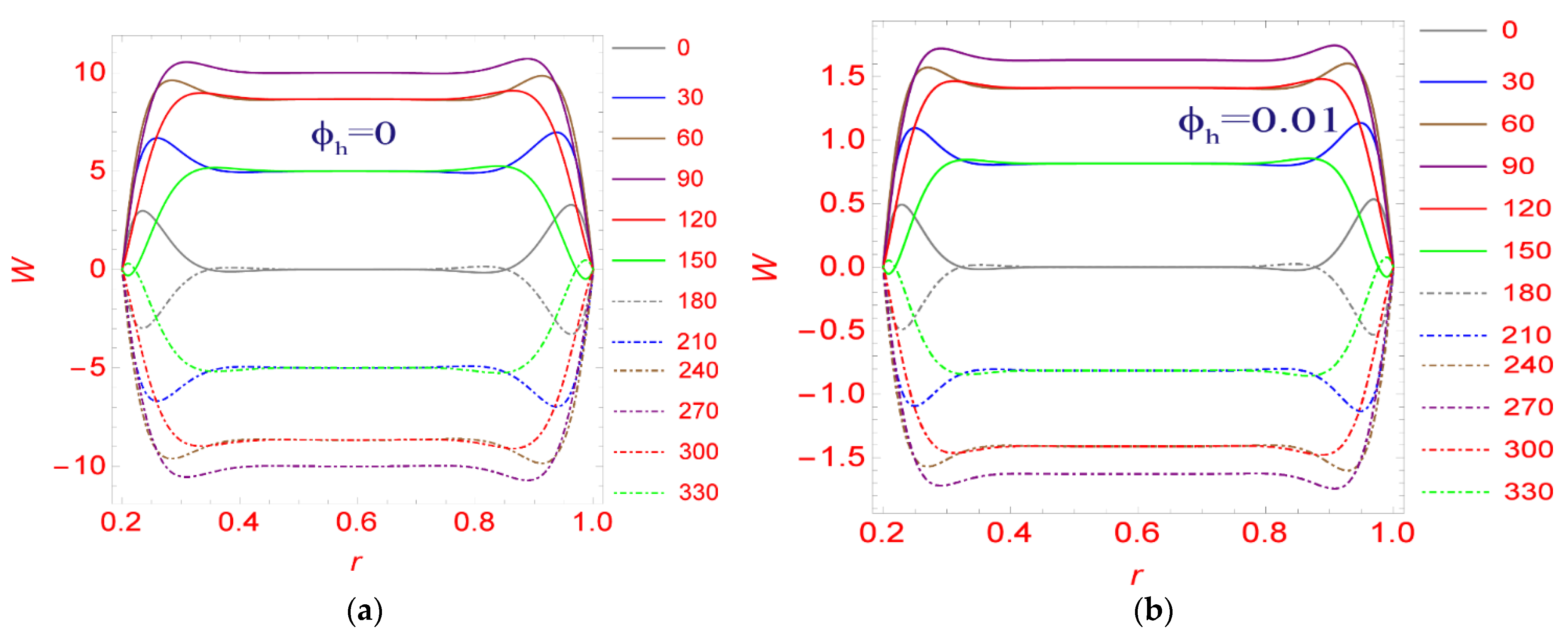
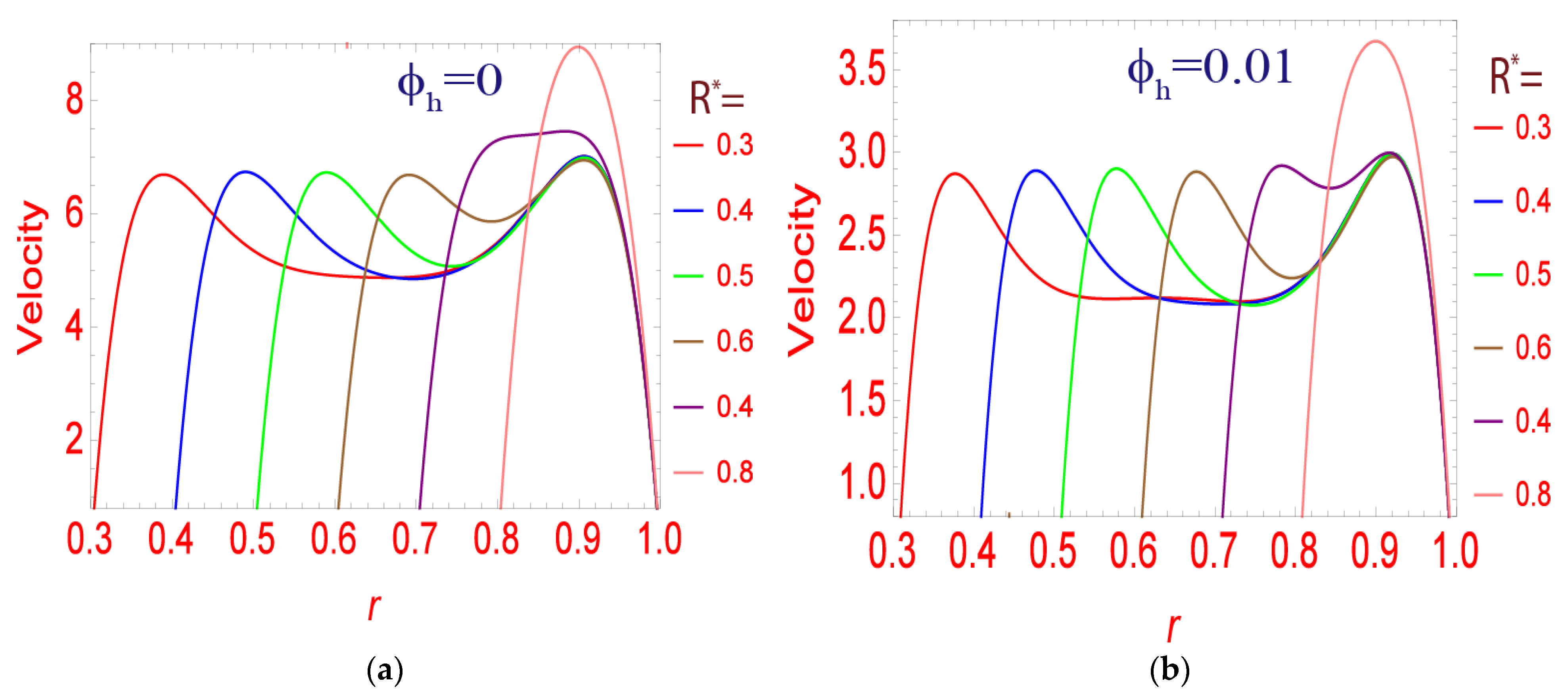
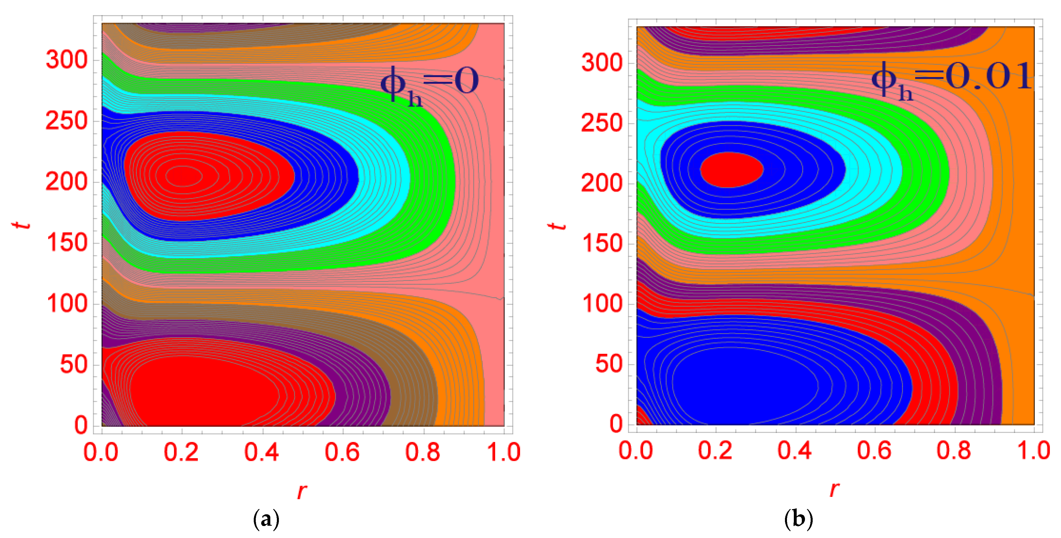
5. Results and Discussion

Numerical calculations of speed profile, temperature profile, vorticity, and stress increase, streamlined to advance an understanding of the physics of the problem, consist of magnetic area parameter M , dynamic Reynolds quantity R e ω , and diverse nanoparticle volumes. Volume fraction, stress gradient vorticity A ¯ , Reynolds quantity Pr, time t, and axial speed are investigated. It varies from inlet to outlet and, because of the improvement of the flow, influences the heat transfer coefficient of a selected area. In a whole pulsation cycle of 360 ° , every example was received at t = 30 ° , and the axial speed version at a given extent fraction ϕ was calculated. All captured times have a completion of 12 in a total pattern of 360 ° . Figure 3a,b show the impact of diverse values of the extent fraction of the nanofluid on the rate profile. Each of those figures suggests that the rate follows an explanatory direction, peaks towards the middle of the channel, and decreases as the extent fraction increases. Furthermore, Figure 3a,b indicate that the addition of nanoparticles increases the overall density of the mixture. In Figure 3a, it may be discovered that there may be a massive and robust perturbation inside the speed profile of the bottom fluid ( ϕ = 0 ) in comparison to the non-0extent fraction of the nanoparticles. Physically adding nanoparticles into blood increases the overall density of the combination greatly. Asa result, as the crossbreed nanofluid thickens, the growth of the mixed nanofluidis slower than that of the base liquid (blood), as seen in Figure 3a,b. Finally, Figure 4a,b show that the most extreme speed of the pulsatile stream is found close to the mass of the channel with fast motions. This is referred to as the ring-like impact and has been tentatively revealed by Richardson et al. [4] who worked with Huq et al. [1]. This ring impact is intensified with the assistance of the Wimberley number R e β . blast. Furthermore, the use of nanoparticles reduces the most extreme speed of the base liquid, as seen in the picture above. The velocity has been proven to diverge somewhat from the mean sinusoidal velocity at a certain instant in time when R e β increases. The annular action increases as R e β increases, the radial velocity near the cylinder wall increases, and the frictional force increases as R e β increases. The inertial component of the momentum equation increases as R e β increases. In addition, increasing the Womersley number raises the speed profile. Because the Womersley number consists of the pulsation to viscous force ratio, raising the Womersley number reduces the viscous force. Then, as the viscous force decreases, the movement of the fluid particles accelerates, resulting in a gradual increase in velocity profile (Figure 5a,b).
Figure 6 is plotted inside the evaluation of Figure 5 for the Hartmann range. In Figure 5, we have inferred that musicality dispersal correlates closely with the assignments of the lines for M = 0 . Regardless, M = 10 beat flow achieves the most prominent ampleness at the recommended limit and signals the logical bearing (Figure 6). It can be observed in Figure 5 and Figure 6 that extension of the Hartmann range affects the sufficiency of the beat profile because of fretful power. In addition, Figure 6a,b show that the helpful asset of the utilization of the expansion of nanoparticles reduces the most extreme rhythm of the least liquid. It very well might be understood from Figure 6 and Figure 7a,b that the attractive issue fills in as a retardant, eventually declining the flowrate. Furthermore, the appealing issue causes the annular effect, which is considered a property of the accepted pulsatile circumstances. The findings of vortex profiles obtained are similar to the results obtained by Majdalani [20]. However, the presence of youngster variants makes explicit the way that Majdalani [20] pushed on a pulsatile coast in a rectangular course. Figure 8a,b show the effect of the volume segment ϕ h on the volume part of vorticity. As indicated by the significance of the vortex, it is a region in a fluid (both genuine and ideal) rotating around a hub line, which may be straight or twisted. Numerically, it is thus far obtained by the twist of a beat problem, and the majority of the time this appropriation/rhythm of liquid is all the more symmetric alongside its pivot. Results introduced in Figure 8 show the unsurprising similarity with the importance of vortex, and it is said that the expense of the vortices is higher at a ludicrous spot in the space. Furthermore, it has been observed that the course of a vortex is pressed with making potential gains of nanoparticle volume part ϕ h (Figure 8a,b). It is likewise cognizant that the vorticity takes awful qualities at heavenly degrees for unmistakable ϕ h values showing the presence of a move to lower accepted circumstances. In an assessment of Figure 8a,b, the model of the vortex can be exceptionally extreme for base liquid ( ϕ h = 0 ) as a study of the nanoparticle volume division.
As shown in Figure 9a,b, the decrease in flow area ends with an increase in velocity. Here, the speed decreases with expanding volume portion ϕ h of the nanoparticles. In Figure 9a,b, the envelope set of the flow domain configuration has achieved the maximum position for increasing the radius value for the various values in the radius and velocity fields. Since the inner radius of the chamber remains precisely or identical to the scope of the outer chamber, we can see that the region of the speed profile is restricted to 0 r 1 , and the greatest speed is close to the channel. As the flow area changes from 0.7 to 1 and the flow area decreases, the annular effect decreases. Research on heat transfer revolves around the research on temperature profiles as well as heat transfer coefficients on walls. Plots are plotted to concentrate on the effect of nanoparticle/Hartmann amount M , stress slope sufficiency, and time at the temperature profile. The amplitude of the stress gradient is plotted in Figure 10a. Note that the temperature profile over the complete variety of two channels decreases because the price of the amplitude stress gradient increases. Figure 10b suggests the adjustments inside the temperature profile plotted in opposition to the Hartmann quantity M inside the Ag-Au/blood hybrid fluid. Because of the lateral magnetic region, the temperature of the fluid rises. Because a magnetic field forms an electric-powered cutting-edge in a liquid, which generates heat, a magnetic field with radiation aids the amplification phenomena. Figure 10c suggests the alternate dimensionless temperature profile of blood-based Ag-Au nanoparticles for distinct quantity fractions ϕ h . It can be shown that as the quantity of nanoparticles increases, so does the heat transmission profile. Based on the high thermal conductivity, it has been shown that primarily blood-based Ag-Au nanoparticles have a higher warmness switch coefficient than the bottom liquid (blood).
In Figure 11, streamlined results are plotted to analyze changes in the flow behavior of Ag-Au nanoparticles on the base fluid and blood. It is possible to see that those streamlines alternate in a sample by identifying the nanoparticles with the extent fraction ϕ h . In the absence of nanoparticles, the contours acquired at ϕ h are less; however, those contours take a much wider form, recognizing the boom inside the extent fraction of the nanoparticle. Figure 11 displays the alternate in strain gradient at the extent fraction of the nanoparticles. The strain gradient is maximized in the middle of the channel at t = 180 ° ; however, a diminishing movement is reached. Be that as it may, at t = 0 ° and t = 360 ° , the strain inclination is insignificant, but a broadened lead improving the expense of ϕ h   can   be   expected . Figure 11b shows changes in the dimensionless temperature profile of a hybrid fluid at various volume fractions ϕ h . From Figure 11a,b, it could be visible that the quantity fraction ϕ modified the heat transfer among two channels because the range of nanoparticles increased. That is, heat transfer is set for the desired application. Figure 12 displays the outcomes of diverse values of quantity fraction ϕ h and time t on pressure gradients. It can be seen that the pressure gradient increases with increasing amount fraction ϕ and time t in the beginning, but then reverses direction at t = 200. There is a period in which the reduction in the pressure gradient dominates with the boost in the volume fraction of nanoparticles, and that is in the range of 100 < t < 300 .

6. Conclusions and Prime Findings

We looked at the effects of utilizing hybrid nanoparticles on blood flow via a problematic artery. The primary goal of this study was to report the CFD results for velocity, temperature, and pressure across the artery’s narrow section. According to the results, the inclusion of gold and silver nanoparticles avoided overheating and favored the maximum velocity. Our simulations might be utilized to provide a more precise picture of hemodynamics. The relationship between speed, stress, and, more importantly, the temperature is shown graphically for expansive degrees of Reynolds number, degree parts, and Hartmann numbers. The following are the study’s concluding remarks fora finer picture of hemodynamics.
Because of the reduction in wave amplitude at high frequencies, the maximum velocity and temperature tend to stay constant.
It is likewise seen that the expansion of Ag-Au hugely expands the temperature of the base liquid.
HNF are more potent coolants than standard base liquids since they can dispose of more warmth than typical base liquids. Because the Womersley number is the ratio of throb to thick powers, an increase in the Womersley number gradually reduces the gooey powers.
It is likewise found that decreasing viscous powers improve the movement of the liquid particles to become quicker, and, therefore, result in a incremental change in the speed profile.
Taking into account viable warm conductivity, it is additionally resolved that blood-based Ag-Au has a higher heat transfer rate when contrasted with the pure fluid.
We may investigate physical properties such as the skin friction coefficient, as well as assess the problem using radiation and magnetohydrodynamic effects to identify the causes of stenosis, which may aid in the treatment of arterial stenosis.
The current technique could be applied to a variety of physical and technical challenges in the future [42,43,44,45,46,47,48,49,50,51,52,53].

Author Contributions

F.S. and W.J. formulated the problem. W.J. and F.A. solved the problem. F.S., W.J., F.A., R.B., E.S.M.T.E.D., H.A.E.-W.K. and A.M.A. computed and scrutinized the results. All authors equally contributed in writing and proofreading of the paper. All authors reviewed the manuscript. All authors have read and agreed to the published version of the manuscript.

Funding

This research received no external funding.

Data Availability Statement

Data will be provided by the authors on request.

Acknowledgments

The researchers would like to thank the Deanship of Scientific Research, Qassim University for funding the publication of this project.

Conflicts of Interest

The authors declare no conflict of interest.

Nomenclature

ρ h n f density of HNF ( K g m 3 )
μ h n f viscosity of HNF ( K g m 1 s 1 )
C h n f specific heat of HNF ( J K 1 k g 1 )
k h n f thermal conductivity of HNF ( W m 1 K 1 )
σ h n f electric conductivity of HNF ( S m 1 )
ρ f density of fluid ( K g m 3 )
ρ p density of NPs ( K g m 3 )
C f specific heat of the fluid ( J K 1 k g 1 )
C p specific heat of NPs ( J K 1 k g 1 )
σ f electric conductivity of fluid ( S m 1 )
σ p electric conductivity of NPs ( S m 1 )
K f thermal conductivity of fluid ( W m 1 K 1 )
K p thermal conductivity of NPs ( W m 1 K 1 )
μ f dynamic viscosity of fluid ( J K 1 k g 1 )
μ p dynamic viscosity of NPs ( J K 1 k g 1 )
α Womersley number ( = R e β   )
γ temperature gradient ( K m 1 )
A Amplitude (m)
ω pulsation
P pressure ( K g m 1 s 2 )
MHartmann number
P r Prandtl number
R e β Reynolds number
t time
D diameter ( m )
r radius ( m )
T temperature ( K )
u , v , w velocity components ( m )
J current density ( A m 1 )
B magnetic field
H magnetic field intensity (T)
C velocity of light ( m s 1 )
L length of the cylinder ( m )
ϕ volume fraction of the nanoparticles
Used Indexes
iinternal
eexternal
ffluid
pparticle

References

  1. Haq, R.U.; Shahzad, F.; Al-Mdallal, Q.M. MHD pulsatile flow of engine oil based carbon nanotubes between two concentric cylinders. Results Phys. 2017, 7, 57–68. [Google Scholar] [CrossRef] [Green Version]
  2. Vardanyan, V.A. Effect of magnetic field on blood flow. Biofizika 1973, 18, 491–496. [Google Scholar]
  3. Richardson, E.G. The amplitude of sound waves in resonators. Proc. Phys. Soc. 1928, 40, 206–220. [Google Scholar] [CrossRef]
  4. Richardson, E.G.; Tyler, E. Transverse velocity gradient near the mouths of pipes in which an alternating or continuous flow of air is established. Proc. R. Soc. London. A 1929, 42, 1–15. [Google Scholar] [CrossRef]
  5. Womersley, J.R. Method for the calculation of velocity, rate of flow and viscous drag in arteries when the pressure gradient is known. J. Physiol. 1955, 127, 553–563. [Google Scholar] [CrossRef]
  6. Uchida, S. The pulsating viscous flow superposed on the steady laminar motion of incompressible fluid in a circular pipe. J. Appl. Math. Phys. 1956, 7, 403–422. [Google Scholar] [CrossRef]
  7. Yang, A.; Chen, L.; Xie, Z.; Feng, H.; Sun, F. Constructal heat transfer rate maximization for cylindrical pin-fin heat sinks. Appl. Therm. Eng. 2016, 108, 427–435. [Google Scholar] [CrossRef]
  8. Cui, X.; Islam, M.; Mohan, B.; Chua, K. Developing a performance correlation for counter-flow regenerative indirect evaporative heat exchangers with experimental validation. Appl. Therm. Eng. 2016, 108, 774–784. [Google Scholar] [CrossRef]
  9. Dhole, A.; Lata, D.; Yarasu, R. Effect of hydrogen and producer gas as secondary fuels on combustion parameters of a dual fuel diesel engine. Appl. Therm. Eng. 2016, 108, 764–773. [Google Scholar] [CrossRef]
  10. Tan, Q.; Hu, Y. A study on the combustion and emission performance of diesel engines under different proportions of O2 & N2 & CO2. Appl. Therm. Eng. 2016, 108, 508–515. [Google Scholar]
  11. Rassoulinejad-Mousavi, S.M.; Seyf, H.R.; Abbasbandy, S. Heat Transfer through a Porous Saturated Channel with Permeable Walls Using Two-Equation Energy Model. J. Porous Media 2013, 16, 241–254. [Google Scholar] [CrossRef]
  12. Rassoulinejad-Mousavi, S.M.; Abbasbandy, S. Analysis of Forced Convection in a Circular Tube Filled With a Darcy–Brinkman–Forchheimer Porous Medium Using Spectral Homotopy Analysis Method. J. Fluids Eng. 2011, 133, 101207. [Google Scholar] [CrossRef]
  13. Rassoulinejad-Mousavi, S.; Porkhial, S.; Layeghi, M.; Nikaeen, B.; Samanipour, H. Experimental study on thermal behavior of a stainless steel-di water flat plate heat pipe. World Appl. Sci. J. 2012, 16, 1393–1397. [Google Scholar]
  14. Seyf, H.R.; Rassoulinejad-Mousavi, S.M. An Analytical Study for Fluid Flow in Porous Media Imbedded Inside a Channel With Moving or Stationary Walls Subjected to Injection/Suction. J. Fluids Eng. 2011, 133, 091203. [Google Scholar] [CrossRef]
  15. Rassoulinejad-Mousavi, S.M.; Abbasbandy, S.; Alsulami, H.H. Analytical flow study of a conducting Maxwell fluid through a porous saturated channel at various wall boundary conditions. Eur. Phys. J. Plus 2014, 129, 181. [Google Scholar] [CrossRef]
  16. Sanyal, D.C.; Biswas, A. Pulsatile motion of blood through an axi-symmetric artery in presence of magnetic field. Assam Univ. J. Sci. Technol. 2010, 5, 12–20. [Google Scholar]
  17. Yakhot, A.; Grinberg, L. Phase shift ellipses for pulsating flows. Phys. Fluids 2003, 15, 2081–2083. [Google Scholar] [CrossRef] [Green Version]
  18. Suces, J. An improved quasi-study approach for transient conjugated forced convection problems. Int. J. Heat Mass Transf. 1981, 24, 711–1722. [Google Scholar]
  19. Latham, T.W. Fluid motions in a peristaltic pump. Master’s Thesis, Massachusetts Institute of Technology, Cambridge, MA, USA, 1966. [Google Scholar]
  20. Majdalani, J.; Chibli, H. Pulsatory Channel Flows with Arbitrary Pressure Gradients. In Proceedings of the 3rd Theoretical Fluid Mechanics Meeting, St. Louis, MO, USA, 24–26 June 2002; p. 2981. [Google Scholar]
  21. Agrawal, H.L.; Anwaruddin, B. Peristalic flow of blood in a branch. Ranchi. Univ. Math. J. 1984, 15, 111–121. [Google Scholar]
  22. Tzirtzilakis, E.E. A mathematical model for blood flow in magnetic field. Phys. Fluids 2005, 17, 077103. [Google Scholar] [CrossRef]
  23. Ramamurthy, G.; Shanker, B. Magneto hydrodynamic effects on blood flow through porous channel. Med. Biol. Eng. Comput. 1994, 32, 655–659. [Google Scholar] [CrossRef] [PubMed]
  24. Mehryan, S.; Sheremet, M.A.; Soltani, M.; Izadi, M. Natural convection of magnetic hybrid nanofluid inside a double-porous medium using two-equation energy model. J. Mol. Liq. 2019, 277, 959–970. [Google Scholar] [CrossRef]
  25. Sidik, N.A.C.; Jamil, M.M.; Japar, W.M.A.A.; Adamu, I.M. A review on preparation methods, stability and applications of hybrid nanofluids. Renew. Sustain. Energy Rev. 2017, 80, 1112–1122. [Google Scholar] [CrossRef]
  26. Xian, H.W.; Sidik, N.A.C.; Aid, S.R.; Ken, T.L.; Asako, Y. Review on preparation techniques, properties and performance of hybrid nanofluid in recent engineering applications. J. Adv. Res. Fluid Mech. Therm. Sci. 2018, 45, 1–13. [Google Scholar]
  27. Ijima, S. Helical microtubules of graphitic carbon. Nature 1991, 354, 56–58. [Google Scholar] [CrossRef]
  28. Cheng, Y.; Zhou, O. Electron field emission from carbon nanotubes. Comptes Rendus. Phys. 2003, 4, 1021–1033. [Google Scholar] [CrossRef]
  29. Timofeeva, E.V.; Routbort, J.L.; Singh, D. Particle shape effects on thermo- physical properties of alumina nanofluids. J. Appl. Phys. 2009, 106, 014304. [Google Scholar] [CrossRef]
  30. Murshed, S.S.; de Castro, C.N.; Lourenço, M.; Lopes, M.; Santos, F. A review of boiling and convective heat transfer with nanofluids. Renew. Sustain. Energy Rev. 2011, 15, 2342–2354. [Google Scholar] [CrossRef]
  31. Jang, J.; Lee, S.S. Theoretical and experimental study of MHD (magnetohydrodynamic) micropump. Sens. Actuators A Phys. 2000, 80, 84–89. [Google Scholar] [CrossRef]
  32. Davidson, P.A. Magnetohydrodynamics in materials processing. Annu. Rev. Fluid Mech. 1999, 31, 273–300. [Google Scholar] [CrossRef]
  33. Choi, S.U.; Eastman, J.A. Enhancing Thermal Conductivity of Fluids with Nanoparticles (No. ANL/MSD/CP-84938; CONF-951135-29); Argonne National Lab (ANL): Argonne, IL, USA, 1995.
  34. Wagner, V.; Dullaart, A.; Bock, A.-K.; Zweck, A. The emerging nanomedicine landscape. Nat. Biotechnol. 2006, 24, 1211–1217. [Google Scholar] [CrossRef] [PubMed]
  35. Fernandez-Fernandez, A.; Manchanda, R.; McGoron, A.J. Theranostic Applications of Nanomaterials in Cancer: Drug Delivery, Image-Guided Therapy, and Multifunctional Platforms. Appl. Biochem. Biotechnol. 2011, 165, 1628–1651. [Google Scholar] [CrossRef] [PubMed] [Green Version]
  36. Yamaguchi, H.; Kobayashi, R.; Takashima, Y.; Hashidzume, A.; Harada, A. Self-Assembly of Gels through Molecular Recognition of Cyclodextrins: Shape Selectivity for Linear and Cyclic Guest Molecules. Macromolecules 2011, 44, 2395–2399. [Google Scholar] [CrossRef]
  37. Mohamed, D.; Abderrahmane, G.; Said, A.; Deghmoum, M.; Ghezal, A.; Abboudi, S. Analytical and numerical study of a pulsatile flow in presence of a magnetic field. Int. J. Phys. Sci. 2015, 10, 590–603. [Google Scholar] [CrossRef] [Green Version]
  38. Jamshed, W. Thermal augmentation in solar aircraft using tangent hyperbolic hybrid nanofluid: A solar energy application. Energy Environ. 2021, 33, 1090–1133. [Google Scholar] [CrossRef]
  39. Deka, R.; Paul, A. Transient free convective MHD flow past an infinite vertical cylinder. Theor. Appl. Mech. 2013, 40, 385–402. [Google Scholar] [CrossRef] [Green Version]
  40. Sobhnamayan, F.; Sarhaddi, F.; Behzadmehr, A. Analytical solution of pulsating flow and forced convection heat transfer in a pipe filled with porous medium. J. Comput. Appl. Mech. 2021, 52, 570–587. [Google Scholar]
  41. Hussain, A.; Sarwar, L.; Rehman, A.; Akbar, S.; Gamaoun, F.; Coban, H.H.; Almaliki, A.H.; Alqurashi, M.S. Heat Transfer Analysis and Effects of (Silver and Gold) Nanoparticles on Blood Flow Inside Arterial Stenosis. Appl. Sci. 2022, 12, 1601. [Google Scholar] [CrossRef]
  42. Huang, J.; Li, Q.; Sun, D.; Lu, Y.; Su, Y.; Yang, X.; Wang, H.; Wang, Y.; Shao, W.; He, N. Biosynthesis of silver and gold nanoparticles by novel sundried Cinnamomum camphora leaf. Nanotechnology 2007, 18, 105104. [Google Scholar] [CrossRef]
  43. Lee, H.-J.; Lee, G.; Jang, N.R.; Yun, J.H.; Song, J.Y.; Kim, B.S. Biological synthesis of copper nanoparticles using plant extract. Nanotechnology 2011, 1, 371–374. [Google Scholar]
  44. Mohanpuria, P.; Rana, N.K.; Yadav, S.K. Biosynthesis of nanoparticles: Technological concepts and future applications. J. Nanoparticle Res. 2008, 10, 507–517. [Google Scholar] [CrossRef]
  45. Rout, B.; Mishra, S. Thermal energy transport on MHD nanofluid flow over a stretching surface: A comparative study. Eng. Sci. Technol. Int. J. 2018, 21, 60–69. [Google Scholar] [CrossRef]
  46. Ren, X.; Meng, X.; Tang, F. Preparation of Ag–Au nanoparticle and its application to glucose biosensor. Sens. Actuators B Chem. 2005, 110, 358–363. [Google Scholar] [CrossRef]
  47. Bhukta, D.; Dash, G.C.; Mishra, S.R.; Jena, S. Analytical estimation of energy dissipations: Viscous, Joulian, and Darcy of viscoelastic fluid flow phenomena over a deformable surface. Heat Transf. 2021, 50, 7798–7816. [Google Scholar] [CrossRef]
  48. Mishra, S.R.; Baag, S.; Parida, S.K. Entropy Generation Analysis on Magnetohydrodynamic Eyring-Powell Nanofluid over a Stretching Sheet by Heat Source/Sink. J. Nanofluids 2022, 11, 537–544. [Google Scholar] [CrossRef]
  49. Mishra, S.R.; Pattnaik, P.; Baag, S.; Bhatti, M.M. Study of kerosene-Gold-DNA nanoparticles in a magnetized radiative Poiseuille flow with thermo-diffusion impact. J. Comput. Biophys. Chem. 2022. [Google Scholar] [CrossRef]
  50. Baag, S.; Mishra, S.R.; Dash, G.C.; Acharya, M.R.; Panda, S. Exact solution for MHD elastico-viscous flow in porous medium with radiative heat transfer. Pramana 2022, 96, 178. [Google Scholar] [CrossRef]
  51. Biswas, R.; Hossain, S.; Islam, R.; Mishra, S.F.A.S.R.; Afikuzzaman, M. Computational treatment of MHD Maxwell nanofluid flow across a stretching sheet considering higher-order chemical reaction and thermal radiation. J. Comput. Math. Data Sci. 2022, 4, 100048. [Google Scholar] [CrossRef]
  52. Mohanty, S.; Mohanty, B.; Mishra, R.S. Analysis of elasticity on the flow of blood through the transient permeable channel with an interaction of radiation. Waves Random Complex Media 2022, 1–18. [Google Scholar] [CrossRef]
  53. Afikuzzaman, M.; Ferdows, M.; Alam, M. Unsteady MHD Casson Fluid Flow through a Parallel Plate with Hall Current. Procedia Eng. 2015, 105, 287–293. [Google Scholar] [CrossRef]
Figure 1. Flow field geometry.
Symmetry 14 02254 g001
Figure 2. Comparison of the velocity profile of the present study with the velocity profile of Mohamed Deghmoum [37] for the different values of t (   M = 10 , R e β = 1 , ϕ h = 0.01 ) .
Symmetry 14 02254 g002
Figure 3. (a) Variation of velocity profile when M = 0 , R e β = 1 , ( ϕ h = 0 ) . (b) Variation of velocity profile when M = 0 , R e β = 1 , ( ϕ h = 0.01 ) .
Symmetry 14 02254 g003
Figure 4. (a) Variation of velocity profile when M = 0 , R e β = 10 , ( ϕ h = 0 ) . (b) Variation of velocity profile when M = 0 , R e β = 10 , ( ϕ h = 0.01 ) .
Symmetry 14 02254 g004
Figure 5. (a) Variation of velocity profile when M = 0 , R e β = 30 , ( ϕ h = 0 ) . (b) Variation of velocity profile when M = 0 , R e β = 30 ,   ( ϕ h = 0.01 ) .
Symmetry 14 02254 g005
Figure 6. (a) Variation of velocity profile when M = 10 , R e β = 1 ,   ( ϕ h = 0 ) . (b) Variation of velocity profile when M = 10 , R e β = 1 ,   ( ϕ h = 0.01 ) .
Symmetry 14 02254 g006
Figure 7. (a) Variation of velocity profile when M = 30 , R e β = 30 , ( ϕ h = 0 ) . (b) Variation of velocity profile when M = 30 , R e β = 30 ,   ( ϕ h = 0.01 ) .
Symmetry 14 02254 g007
Figure 8. (a) Variation of vortex profile t for Pure fluid ( ϕ h = 0 ) when R e β = 10 ,   M = 5 . (b) Variation of vortex profile t for hybrid fluid ( ϕ h = 0.01 ) when R e β = 10 ,   M = 5 .
Symmetry 14 02254 g008
Figure 9. (a) Variation of a velocity profile for various values of   R * when ( ϕ h = 0 ) . (b) Variation of a velocity profile for various values of   R * when ( ϕ h = 0.01 ) .
Symmetry 14 02254 g009
Figure 10. (a) Variation of temperature profile for various values of pressure gradient A . (b) Variation of temperature profile for various values of Hartmann number M . (c) Variation of temperature profile for various values of nanoparticles ϕ h .
Symmetry 14 02254 g010
Figure 11. (a) Streamlines for pure fluid ( ϕ h = 0 ) . (b) Streamlines for Ag-Au/blood hybrid fluid for ( ϕ h = 0.01 ) .
Symmetry 14 02254 g011
Figure 12. Pressure gradient for when A ¯ = 20 , M = 10 , α = 10 and R * = 0.2 .
Symmetry 14 02254 g012
Table 1. Thermo-physical features of hybrid nanofluid [38].
FeaturesHybrid Nanofluid
Viscosity ( μ ) μ h n f = μ f ( 1 ϕ A ) 2.5 ( 1 ϕ B ) 2.5
Density   ( ρ ) ρ h n f = [ ( 1 ϕ B ) { ( 1 ϕ A ) ρ f + ϕ A ρ p 1 } ] + ϕ B ρ p 2
Heat   capacity   ( ρ C p ) ( ρ C p ) h n f = [ ( 1 ϕ B ) { ( 1 ϕ A ) ( ρ C p ) f + ϕ A ( ρ C p ) p 1 } ] + ϕ B ( ρ C p ) p 2
Thermal   conductivity   ( κ ) κ h n f κ g f = [ ( κ p 2 + 2 κ g f ) 2 ϕ B ( κ g f κ p 2 ) ( κ p 2 + 2 κ g f ) + ϕ B ( κ g f κ p 2 ) ] ,
κ g f κ f = [ ( κ p 1 + 2 κ f ) 2 ϕ A ( κ f κ p 1 ) ( κ p 1 + 2 κ f ) + ϕ A ( κ f κ p 1 ) ]
Electrical   conductivity   ( σ ) σ h n f σ f = [ 1 + 3 ( ϕ A σ p 1 + ϕ B σ p 2 σ f ( ϕ A + ϕ B ) ) ( ϕ A σ p 1 + ϕ 2 σ p 2 ( ϕ A + ϕ B ) σ f + 2 ) ( ϕ A σ p 1 + ϕ B σ p 2 σ f ( ϕ A + ϕ B ) ) ]
Table 2. Thermophysical properties.
Thermophysical ρ ( k g / m 3 ) c p ( J / k g K ) σ ( Ω   m ) k ( W / m K ) P r
Blood106335940.6670.49221
Silver (Ag)10,5002356.3 × 10 7 429-
Gold (Au)19,2821294.1 × 10 6 310-
Publisher’s Note: MDPI stays neutral with regard to jurisdictional claims in published maps and institutional affiliations.

