Article

Analysis of MHD Falkner–Skan Boundary Layer Flow and Heat Transfer Due to Symmetric Dynamic Wedge: A Numerical Study via the SCA-SQP-ANN Technique

by
Kamsing Nonlaopon
1,
Muhammad Fawad Khan
2,
Muhammad Sulaiman
2,*,
Fahad Sameer Alshammari
3 and
Ghaylen Laouini
4
1
Department of Mathematics, Faculty of Science, Khon Kaen University, Khon Kaen 40002, Thailand
2
Department of Mathematics, Abdul Wali Khan University, Mardan 23200, Pakistan
3
Department of Mathematics, College of Science and Humanities in Alkharj, Prince Sattam Bin Abdulaziz University, Al-Kharj 11942, Saudi Arabia
4
College of Engineering and Technology, American University of the Middle East, Egaila 54200, Kuwait
*
Author to whom correspondence should be addressed.
Symmetry 2022, 14(10), 2180; https://doi.org/10.3390/sym14102180
Submission received: 24 August 2022 / Revised: 25 September 2022 / Accepted: 9 October 2022 / Published: 17 October 2022

Abstract

:
This article considers Falkner–Skan flow over a dynamic and symmetric wedge under the influence of a magnetic field. The Hall effect on a magnetic field is negligible for small magnetic Reynolds numbers. The magnetic field B ( x ) is considered over x-axis, which is in line with the wedge i.e., parallel, while the flow is transverse over the y-axis. This study has numerous device-centric applications in engineering, such as power generators, cooling reactor and heat exchanger design, and MHD accelerators. The Third and second-ordered ordinary differential equations characterize the system. A novel hybrid computational technique is designed for the surrogate solutions of the Falkner–Skan flow system. The designed technique is based on the sine–cosine optimization algorithm and sequential quadratic programming. Reference solutions are calculated by using the Runge–Kutta numerical technique. Performance matrices evaluate the accuracy and stability of our surrogate solutions, mean-absolute deviation (MAD), root-mean-square error (RMSE), and error in Nash-–Sutcliffe efficiency (ENSE). Furthermore, graphical representations in terms of convergence graphs, mesh graphs, stem graphs, stairs plots, and boxplots are presented to establish the symmetry, reliability, and validity of our solutions.

1. Introduction

The boundary layer flows have many applications in different field of study such as engineering, physics, acoustics, etc.; therefore, the boundary layer flow attracts the interest of researchers. The Falkner–Skan flow is investigated in this article, which was presented by Falkner and Skan [1]. With the help of this flow, they illustrate the functions of Prandtl’s theory about boundary layer flows. Extensive research work was performed on Falkner–Skan flow (FSF). First, this was considered an abstract concept; later on, it was discussed as a benchmark. It was discussed through various aspects, analytically by Barania [2] and numerically by Howarth [3] and Barania [4]. Many tools, such as power machine, heat exchanger design, cooling of reactors, and magnetohydrodynamic accelerators are based on the applications of magnetohydrodynamic (MHD) incompressible viscous flow. Many researchers had worked on MHD incompressible flow including Sayyed et al. [5] and Abbasbandy and Hayat [6]. Abbas et al. [7] investigated a Maxwell fluid flowing in a porous channel with MHD boundary layers. Mukhopadhyay [8] studied a heated stretched sheet with changing viscosity and with MHD boundary layer flow. Khazayinejad and Naurazar [9] studied the impact of spatial fractional heat conduction by employing a Gr-Fe3O4—H2O hybrid nanofluid in MHD boundary layer flow. Anusha provided an analytical study of MHD Marangoni boundary layer flow and heat transfer with mass transpiration and radiation [10]. Guo reported granular flow heat transfer in a movable bed around a tube bank that is aligned—experimental investigation and theoretical forecasting using a thermal resistance model [11]. B Shankar [12] discussed the impact of thermal radiation and joule heating on the MHD boundary layer of nanofluid flowing along an exponentially extending surface. T Anusha [13] studied mass transpiration and the Brinkman ratio in nanofluid flow with MHD over a porous stretching and contracting plate. EM Elsaid [14] performed a 3D sinusoidal cylinder hybrid nanofluid MHD boundary layer analysis. Cui presented the thermal performance of composite phase-change materials made of modified melamine foam, graphene, and paraffin wax for solar thermal energy storage and conversion [15]. P Rai [16] investigated the boundary layer flow over a moving plate with a magnetic field present and slip conditions. Yaseen et al. in [17], studied the Falkner–Skan problem for shrinking and stretching edges. They developed a generalized model to study the nanoparticle aggregation effect. The model considered the magnetic field suction/injection and thermo/radiation for the prediction of T 1 O 2 / E G nanofluid. R Garia et al. [18] scrutinized the hybrid nanofluid flow of S i O 2 M o S 2 / w a t e r —the study was extended in two different geometries: a wedge and a cone. L Ali [19] provided an analysis of the chemical reaction and Cattaneo–Christov heat flux model for the bio-convective MHD Blasius and Sakiadis flow. C Ram Reddy [20] studied dual solutions for inclined magnetohydrodynamics and Joule effects in Ti-alloy nanofluid flow separation, and investigated their stability.
In this study, the MHD incompressible flow is studied on a movable wedge. This phenomenon has several applications in engineering problems, such as hydrodynamics, aerodynamics, and automotive engineering. Siddique et al. [21] presented biofuel applications in the bioconvection of MHD flow over a sheet being stretched exponentially. Das and Wang [22] elucidated specific uses for MHD pump flows in diagnostic device design and fabrication. The viability of MHD ship propulsion utilizing superconductive magnets was examined in light of developments in high-temperature superconductivity. Consequently, a current analysis of the advancements made in MHD pump applications is required. It was previously studied by Kudenatti [23] discussing 2D magnetohydrodynamic boundary layer flow (BLF) over an approximately infinite flat plate. Ishak et al. discussed MHD-BLF past a moving wedge [24]. Falkner–Skan BLF problems are modeled by nonlinear third-order differential equations. Bagh et al. [25] evaluate fluid by With the use of a finite element simulation, the magnetic and bio-convection effects on the tangent hyperbolic nanofluid flow through a faster/slower stretching wedge were aligned.
It was solved numerically [26] as well as analytically. An analysis of a marine engine’s transient performance in a simulation when coupled with an SCR system at high pressure is reported in [27]. Habib et al. [28] numerically investigated, due to a sliding wedge, MHD Prandtl nanofluid transportation: Keller box approach. Habib et al. also discussed the importance of mass transpiration and bioconvection in MHD micro-polar Maxwell nanofluid flow across an expanding sheet [29]. Guo et al. talked about how the inclination of the tube affected heat transfer in gravity-driven granular flow around the tube out-wall [30]. Analytically, the perturbation method was used by Barania [2] and a good technique for the optimal homotopy asymptotic method (OHAM) was presented and evaluated by Marinca and Herişanu [31]. Ali et al. discussed the buoyancy effects on the wedge that is passed by a Maxwell nanofluid fluid in a Falkner–Skan flow using a finite element method [32]. Bejan’s [33] analysis of heat transfer in terms of thermodynamic processes intended to upgrade caloric systems by boosting heat transmission and lowering drop in pressure; the researcher found that minimizing entropy production might improve the thermal system’s engineering design. The extreme drop of irreversibility, associated with mass transfer, heat transfer, viscosity lowering or dissipation, magnetic field, chemical phenomena, and so on, maybe demonstrated methodically by minimizing the overall entropy production. Entropy creation because of the heat transfer in the MHD boundary flow has been examined by several researchers. Makinde [34], for example, looked at the formation of entropy inside an MHD-BLF and heat transmission over a convective surface on a flat plate. Butt and Asif [35] used a stretched porous sheet in a porous environment to examine entropy formation in MHD flow. Entropy production radiation-driven nanofluid flow a magnetic field across a porous plate was numerically explored by Dehsara et al. [36]. The MHD was used by Yazdi et al. [37] to investigate the entropy creation of parallel open micro-channels embedded into a moving absorbent surface, and Fawad et al. [38] investigate the characteristic of Falkner–Skan flow over a dynamic wall having mass transfer and gradient of pressure along a stream.
Despite the numerical and analytical solutions, the solutions of the differential equation model by stochastic technique has grabbed the interest of researchers. The stochastic technique uses an artificial neural network for approximating the solution. These solutions were more promising and reliable as compared to other numerical and analytical solutions. These techniques are implemented in various fields, including engineering, biomathematics, physics, heat transfer, etc. The biomathematics problem of virotherapy for cancer was modeled and analyzed using a neuro-hybrid computing technique reported in [39]. Cui, using numerical simulation and an artificial neural network, detailed the heat transport of a phase change material composited with a metal foam-fin hybrid structure in an inclined container [40]. Huang reported the mixing behavior of hot and cold fluids in a rectangular T-junction with or without an impeller, and provided a numerical simulation [41]. The heat transfer problem is solved by [42], who employed a novel-hybrid neural-soft computing-based quantitative analysis of the non-linear convective heat transfer model, using a new soft computing technique. In the study of beam-column configurations with varying axial loads, internal forces, and bending rigidity [43], a hybrid meta-heuristic using neuro-computing for unipolar analysis electro-hydrodynamic pump flow [44], and wire coating procedure with Oldroyd constant fluid analyzed by the soft computing technique was presented in [45].
Despite the significant influx of new methods in this field, it is still unclear whether or not we require further techniques. The so-called no free lunch (NFL) theorem can provide an answer to this question [46]. This theorem logically demonstrates that no one is capable of proposing an algorithm for resolving all problems. This implies that an algorithm’s success in addressing a particular set of problems does not imply that it will be successful in tackling all problems of all types and backgrounds. In other words, regardless of the higher performance on a subset of problems, all techniques perform equally when taking into account all of the problems. With the help of the NFL theorem, researchers may suggest brand-new optimization algorithms or enhance/modify the ones that are already in use to address specific problem subsets in various domains.
This is also the motivating factor for this study, which proposes the simplest, yet efficient, optimization strategy to solve optimization problems involving unknowable search spaces. The study demonstrates that a meta-heuristic does not always require a real-world example as inspiration, and that optimization methods in this area may be designed using basic mathematical operations. In an attempt to find better solutions, the suggested algorithm employs the use of the sine and cosine functions for exploration and exploitation in the search space. The objective of this study was to investigate heat transmission by a moving wedge inside an MHD boundary layer flow. The impacts of parameters such as magnetic field and velocity ratio are considered. The problem is solved by a novel developed hybrid soft-computing technique. In this work, sine–cosine algorithm (SCA), a global search technique, sequential quadratic programming (SQP), and a local search technique are hybridized for the solution of the FSBLF problem. The novel hybrid technique uses an artificial neural network (ANN) for approximating the numerical solution of FSF. The technique is named SCA-SQP-ANN throughout the study. The salient features of the work are as follows:
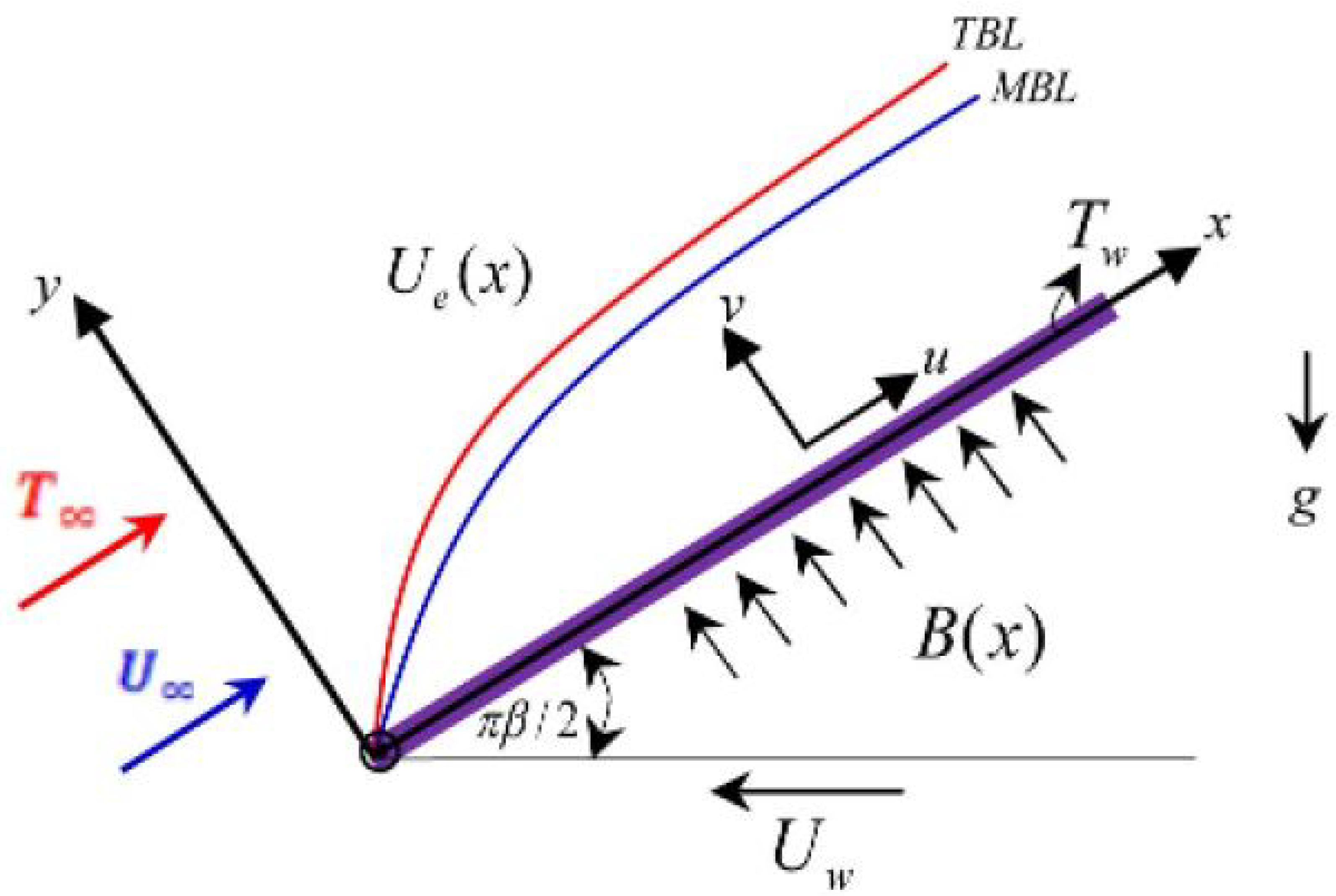
  • Provide an investigation of heat transmission by a moving symmetric wedge inside an MHD Falkner–Skan boundary layer flow (FSBLF).
  • A magnetic field that effects and the velocity–ratio parameter is taken into account.
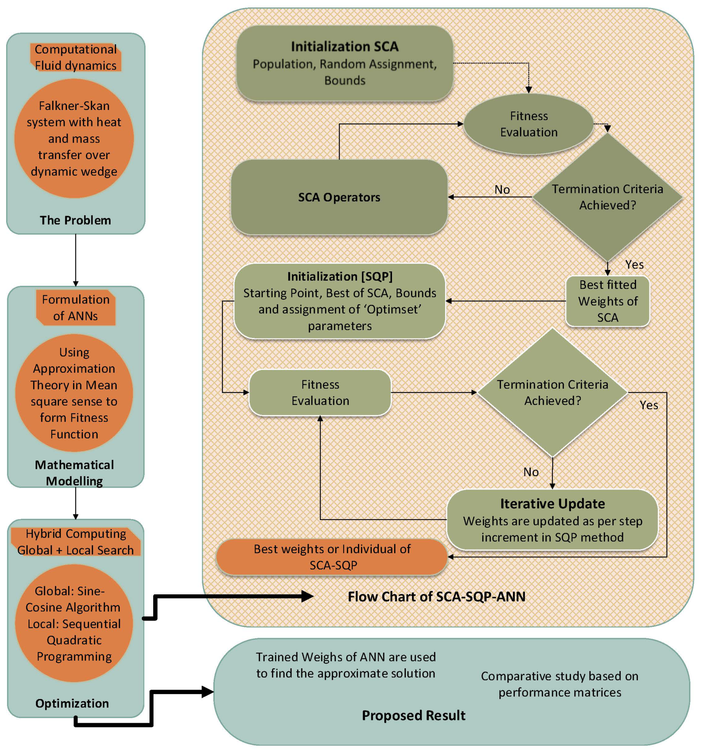
  • For the surrogate solutions of FSBLF, a novel hybrid machine learning technique SCA-SQP-ANN is developed.
  • Validation, training, and testing are carried out for different cases of FSBLF.
  • The surrogate solutions are obtained using SCA-SQP-ANN and the results are discussed and symmetries are studied using graphical and statistical representations.
The rest of the paper is arranged as follows: Section 2 presents the mathematical derivation of MHD FSBLF; Section 3 presents the procedure for the solution of FSBLF; Section 4 presents graphical and empirical discussion on the solution of SCA-SQP-ANN and Section 5 concludes the work.

2. Mathematical Formulation

A symmetric moving wedge is used to create a two-dimensional (2D) MHD flow. For tiny magnetic Reynolds numbers, hall-induced magnetic fields are minimal. B ( x ) is the applied magnetic field. The velocities of the free stream U e and wedge U w are indicated by U x m and U w x m , respectively. The problem yields the given equations: [25,29,32,47]
u x + v y = 0 ,
u u x + v u y = U U e x + μ ρ 2 u y 2 σ B 2 ( x ) ρ u U e ,
u T x + v T y = α 2 T y 2 + μ ρ c p u y 2 ,
where u is x component and v is y component of the velocity of the fluid flow. In addition, μ is the fluid’s dynamic viscosity, ρ is density, α is thermal diffusivity, ρ c p is heat capacitance and electrical conductivity is denoted by σ , B ( x ) = B 0 x ( m 1 ) / 2 is the magnetic field in x direction. The conditions at the boundaries of Equations (1)–(3) are as follows:
u = U w ( x ) = U w x m , v = 0 , T ( 0 ) = T w , u = U e ( x ) = U x m , v = 0 , T ( ) = T ,
to transform the model into ordinary differential equations, the following transformations are implemented [25]:
h = y ( m + 1 ) U e ( x ) 2 v x , u = U e ( x ) f ( η ) , θ = T T T w T v = ( m + 1 ) 2 v U e ( x ) x f + m 1 m + 1 η f ( η ) ,
where prime denotes derivative with respect to η . Placing Equation (5) into Equations (2)–(4) produces the following:
f ( η ) + f ( η ) f ( η ) + β 1 f ( η ) 2 + M 2 1 f ( η ) = 0 ,
θ ( η ) + Pr f ( η ) θ ( η ) + B r f ( η ) 2 = 0 .
The subjected non-dimensional boundaries are:
f ( 0 ) = 0 , f ( = 0 ) = λ , θ ( 0 ) = 1 , f ( 1 ) = 1 , θ ( 1 ) = 0 .
The nonlinear pressure gradient β , the Prandtl number Pr, the magnetic parameter, also known as the Hartman number M, the Brinkman number is defined as B r = P r E c , where E c is the Eckert number, and the velocity ratio parameter λ is the non-dimensional constant in Equations (6)–(8). The definitions of these parameters are given below:
β = 2 m m + 1 , M = B 0 2 2 σ x / ρ U e ( m + 1 ) , Pr = v α B r = μ U e 2 k Δ T , E c = U e 2 c p Δ T , λ = U e U w .
For λ > 0 shows the moving in same direction and λ < 0 show the moving wedge is in opposite directions to the free stream. Moreover, λ = 0 represents the stationary wedge. Similarly, β > 0 shows favorable pressure gradients to the wedge and β < 0 show negative pressure gradients. The physical structure in coordinate system is given in Figure 1.

3. Design Methodology

The suggested designed scheme for the Falkner–Skan heat transfer model (FS-HTM) solution is covered in this section. An ANN is used to construct the methodology. Here, the mathematical model based on ANN is created for the FS-HTM, and the fitness of the model’s solutions is determined using the least square errors in the fitness function.

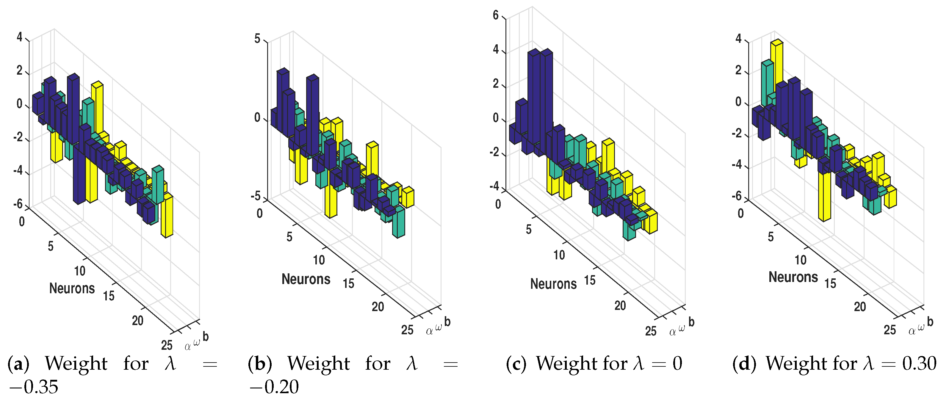
3.1. Transformation of FS-HTM to ANN

In order to solve the FS-HTM model, the model is created using a feed-forward artificial neural network. This kind of ANN only has one direction. There is no cycle formed by the layer. Since ANN is based on an activation function, all information travels along a single channel from node to node. In this work, the FS-HTM model’s approximate solution is determined by the log–sigmoid activation function. The model proceeds as:
f ^ ( η ) + f ^ ( η ) f ^ ( η ) + β 1 f ^ ( η ) 2 + M 2 1 f ^ ( η ) = 0 ,
θ ^ ( η ) + Pr f ^ ( η ) θ ( η ) + B r f ^ ( η ) 2 = 0 ,
f ^ ( η ) = i = 1 k a f i ϕ w f i ( η ) + b f i f ^ ( η ) = i = 1 k a f i ϕ w f i ( η ) + b f i f ^ ( η ) = i = 1 k a f i ϕ w f i ( η ) + b f i E ^ ( n ) ( η ) = i = 1 k a E i θ ( n ) w E i ( η ) + b E i ,
θ ^ ( η ) = i = 1 k a θ i ϕ w ϕ i ( η ) + b θ i θ ^ ( η ) = i = 1 k a θ i ϕ w θ i ( η ) + b θ i θ ^ ( η ) = i = 1 k α θ i ϕ w ϕ i ( η ) + b θ i ϕ ^ ( n ) ( η ) = i = 1 k α θ i ϕ ( n ) w θ i ( η ) + b θ i ,
Equations (12)–(13) are an ANN model for the approximation of fand θ and their respective derivatives. The system is designed by the activation function given in Equation (14) and by substituting ANN weights, Equation (14) obtains the shape given in Equation (15) and Equation (16) is its derivative.
ϕ ( x ) = 1 1 + e x ,
ϕ ^ ( η ) = i = 1 k a i 1 1 + e ω i η + b i ,
ϕ ^ ( η ) = i = 1 k a i ω i e ω i η + b i 1 + e ω i η + b i 2 ,
Equations (15) based on variables of ANN called weights (W) as W = [ a i , w i , b i ] , where ω i = w 1 , ω 2 , . ω k a i = a 1 , a 2 , . a k , and b i = b 1 , b 2 , . b k .

3.2. Fitness Function

Using mean square errors (MSE), the fitness function for the FS-HTM system is created as follows:
e = e f + e θ + e c ,
where e f and e θ are cost functions of the system (10) and (11), respectively, as:
e f = 1 N m = 1 N f ^ ( η ) + f ^ ( η ) f ^ ( η ) + β 1 f ^ ( η ) 2 + M 2 1 f ^ ( η ) 2 , η ( 0 , 1 ) ,
e θ = 1 N m = 1 N θ ^ ( η ) + Pr f ^ ( η ) θ ( η ) + B r f ^ ( η ) 2 2 , η ( 0 , 1 ) ,
where N = 1 h , step size in given span is h. Error function e c is connected to the following initial conditions:
e c = 1 5 f ^ 0 2 + f ^ 0 2 + θ ^ 0 1 2 + f ^ 1 1 2 + θ ^ 1 2 .

3.3. Optimization Procedure

To assess the FS-HTM model’s dynamic behavior, the system is altered to become an optimization problem. Where a fitness function based on MSE is established. The definition of the fitness function is given in Equation (17). The solution to the FS-HTM problem is evaluated based on fitness values. For the optimization of the fitness function, a novel hybrid optimization procedure is introduced. The hybrid technique is based on local search and global search optimization procedures. For global search, sine–cosine algorithm (SCA) is used. The SCA investigates the space of potential optimal values and these values are assigned as an initial point to local search technique sequential quadratic programming (SQP). The SCA was initially presented by Mir Jalili. The SCA is a population-based method motivated by trigonometric functions sine and cosine. It generates a collection of arbitrary solutions and compares them to obtain the best one. For the performance evaluation of SCA, about nineteen composite functions were solved and the results were compared with the results of the genetic algorithm, particle swarm optimization, bat algorithm, flower pollination algorithm, firefly algorithm, and gravitational search algorithm [48]. The results were comparatively better. The reliability and consistency of SCA is tested on many problems, such as designing bend photonic crystals [49], the construction duration and schedule robustness was solved by [50], hydro-thermal-wind scheduling [51], automatic regulation voltage system set up [52], wind plant energy production [53], etc. To improve the exploitation of SCA, it is hybridized with the rapid convergence local search technique SQP and feed-forward neural network. It has many applications in solving problems, such as time-domain radiant transfer, which determines how optical parameters are distributed [54], control allocation with singularity avoidance [55], power system optimal power flow solutions [56], elitist feature selection with a new update mechanism [57], models of nonlinear electric circuits using computational intelligence [58], etc. The designed technique is abbreviated as SCA-SQP-ANN. For validity, reliability, and consistency, the solution of Runge–Kutta order 4 (RK4) is used as a benchmark solution. Figure 2 presents the flow chart for the optimization process.

3.4. Performance Operators

To verify and assess how well the suggested paradigm, SCA-SQP-ANN, works, operators for statistical performance are employed. The performance metrics used, such as Nash–Sutcliffe efficiency, are mean absolute deviation (MAD), root-mean-squared error (RMSE), and error in Nash–Sutcliffe efficiency (ENSE). For each variable in the model, performance operators are defined. The description of performance metrics may be seen in the following mathematical formulations:
MAD f MAD θ = 1 m i = 1 m f i f ^ i 1 m i = 1 m θ i θ ^ i ,
RMSE f RMSE θ , = 1 m i = 1 m f i f ^ i 2 1 m i = 1 m θ i θ ^ i 2 ,
[ NSE f NSE θ ] = 1 i = 1 m f i f ^ i 2 i = 1 m f i f ¯ i 2 1 i = 1 m θ i θ ^ i 2 i = 1 m θ i θ ¯ i 2 ,
ENSE f ENSE θ = 1 N S E f 1 N S E θ .
In Equations (21)–(23), m is number of input depending on the choice of step size, f , and θ , are reference solutions found by RK4 and f ^ and θ ^ are numerical solutions carried out using the SCA-SQP-ANN approach. The ideal answers return 0 for MAD, RMSE, and ENSE. The worth of NSE determines the worth of ENSE. NSE has a value of 1. While the value of NSE approaches 1, the value of ENSE moves away from 1 and toward 0. It shows that the SCA-SQP-ANN method has converged. Additionally, the global operators of MAD, RMSE, and ENSE are abbreviated as GMAD, GRMSE, and GENSE. The following are the definitions for the global variant:
GMAD f GMAD θ = 1 R i = 1 R 1 m k = 1 m f i f ^ i 1 R i = 1 R 1 m k = 1 m θ i θ ^ i ,
GRMSE f GRMSE θ = 1 R i = 1 R 1 m k = 1 m f i f ^ i 2 1 R i = 1 R 1 m k = 1 m θ i θ ^ i 2 ,
GENSE f GENSE θ = 1 R i = 1 R 1 k = 1 m f i f ^ i 2 k = 1 m f i f ^ i 2 1 R i = 1 R 1 k = 1 m θ i θ ^ i 2 k = 1 m θ i θ ^ i 2 .
In Equations (25)–(27), R indicates the SCA-SQP-ANN technique’s number of executions (or runs). The average value of each operator affects the values of GMAD, RMSE, and GENSE.

4. Empirical Simulation and Results

Falkner–Skan BLF with heat and mass transfer over a dynamic wedge under the impact of a magnetic field is categorized into two problems. In the first problem, the velocity ratio parameter is used to examine the dynamic wedge in both the same and opposing directions to the free stream. If λ < 0 , the moving wedge is in the opposite direction, while for λ > 0 , the moving wedge is in the same direction to the free stream. Further, for λ = 0 the wedge is stationary. In the second problem, various magnetic field strengths are tested.

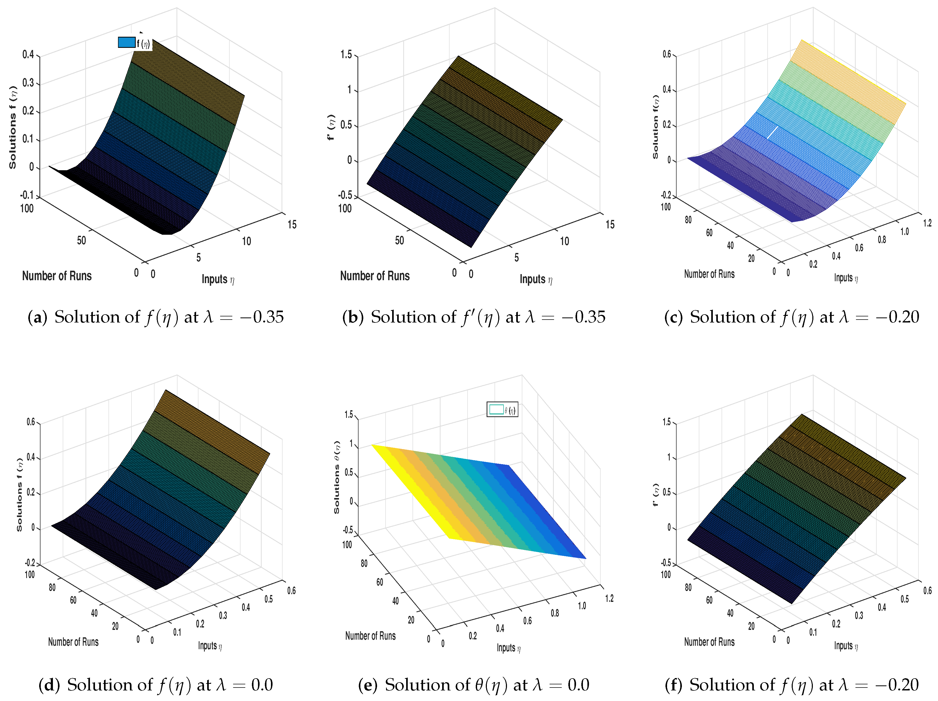
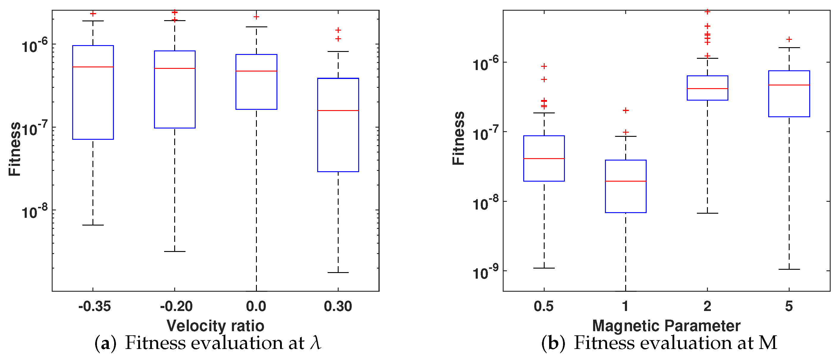
4.1. Problem 1: Variation in Velocity Ratio λ

This problem is based on the variation in the velocity ratio parameter ( λ ). The values of parameters are P r = 0.72 , B r = 0.1 , M = 1.0 , β = 0.4 and λ = 0.35 , 0.20 , 0 , 0.30 . The variation in values of λ creates four cases in this problem. For λ > 0 , the wedge is moving in the same direction, and when λ < 0 , the moving wedge is in opposite directions to the free stream; λ = 0 represents a stationary wedge. The problem is solved by SCA-SQP-ANN. The obtained solution by the SCA-SQP-ANN algorithm is drawn against the reference solution of Runge–Kutta order four. The cross referencing of solutions of the suggested technique with reference solution validates the solution. The graphs of all four cases are plotted in Figure 3. Furthermore, the execution of the SCA-SQP-ANN algorithm is assessed using statistical terminology mean, standard deviation (STD), and minimum (MIN).
In Figure 3, all the variations of the velocity ratio λ is drawn against the solution of RK4. It is seen that the solution of the SCA-SQP-ANN algorithm and RK4 overlapped. This indicates the validation of solutions of the SCA-SQP-ANN algorithm. The numerical solution of the RK4 and SCA-SQP-ANN algorithms are given in Table 1 and Table 2. The solutions of the SCA-SQP-ANN algorithm are based on the variables of ANN called weights. The values of weights are drawn using a 3D bar graph given in Figure 4a–d. The weights are trained in the interval [ 5 , 5 ] . These are ten sets of triplets, named W i = { α i , ω i β i } . Each color represents α , ω , and β , respectively. The solution to the problem is acquired by substituting weights that have been trained by ANN in the Equation (15). The solutions are given in Appendix A in Equation (A1)–(A4) with 14-digit precision.

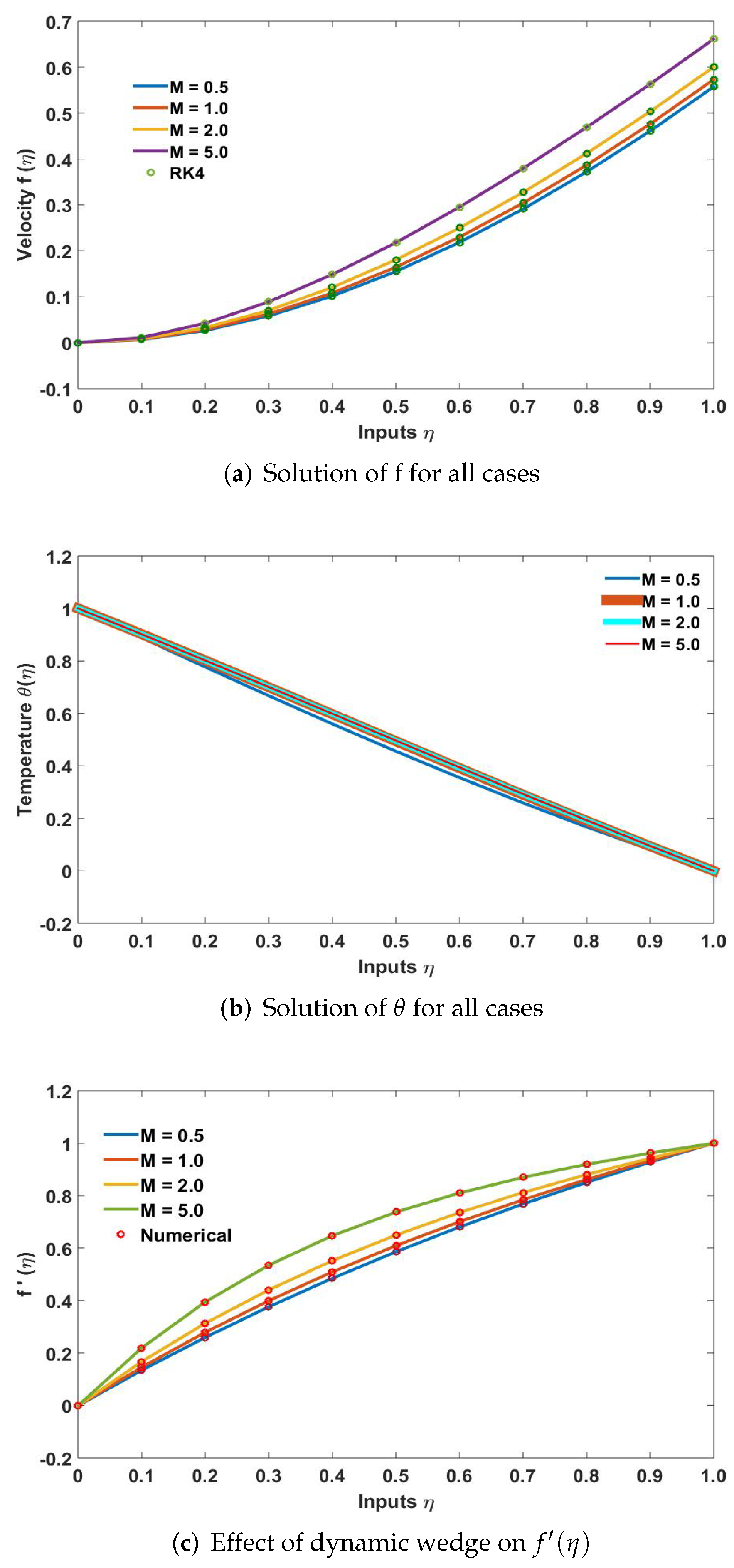
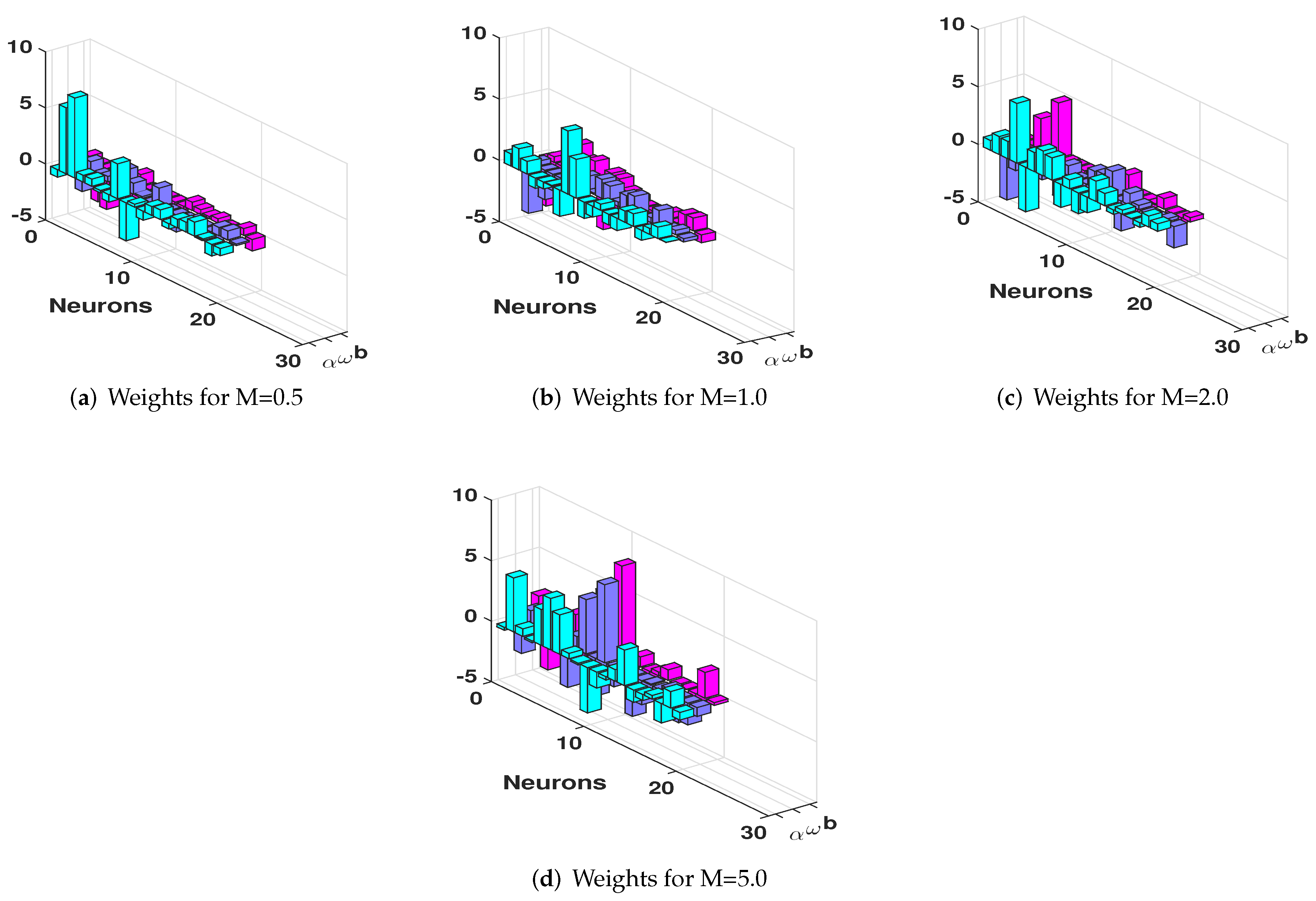
4.2. Problem 2: Variation in Magnetic Parameters M

This problem is based on the variations of magnetic parameters or Hartman number (M). The values of parameters are P r = 0.72 , β = 0.5 , B r = 0.1 and λ = 0 . The magnetic parameter varies with values M = 0.5 , 1 , 2 , and 5. The variation in magnetic parameters creates four cases in this problem. The problem is solved by the SCA-SQP-ANN algorithm. The obtained solution of SCA-SQP-ANN algorithm is drawn against the reference solution of Runge–Kutta order four. The validation of the solution comes from the suggested technique, by overlapping solutions with the reference solution. The graphs of all four cases are plotted in Figure 5. In Figure 5, it can be observed that velocity increases with the increase in magnetic parameters, because the magnetic field produces a Lorentz force, which provides additional kinetic energy (KE) to the particles of the fluid, due to which, the velocity increases. Additionally, the SCA-SQP-ANN’s performance is assessed using the statistical concepts of mean, standard deviation (STD), and minimum (MIN).
The overlapping of solution of the RK4 and SCA-SQP-ANN algorithm validates the obtained solution of SCA-SQP-ANN. The solution of the SCA-SQP-ANN algorithm is based on the trained variable of ANN called weights. The values of weights are drawn using 3D bar graph given in Figure 6. The weights are trained in the interval [ 5 , 5 ] . These are ten sets of triplet named as W i = { α i , ω i , β i } . Each color represent α , ω , and β , respectively. By substituting these weights in Equation (15) gives the solution to the problem. The expended form of solution is provided in Appendix A with a 14-digit precision.
Additionally, the parameter pressure gradient ( β ) is varies. The graphs of temperature and velocity profile for β = 0.1 , 1 , 2 , 4 is given in Figure 7. It can observe that the temperature profile is not much varies with the values of β . While, the velocity increases with increase in pressure gradient ( β ) .

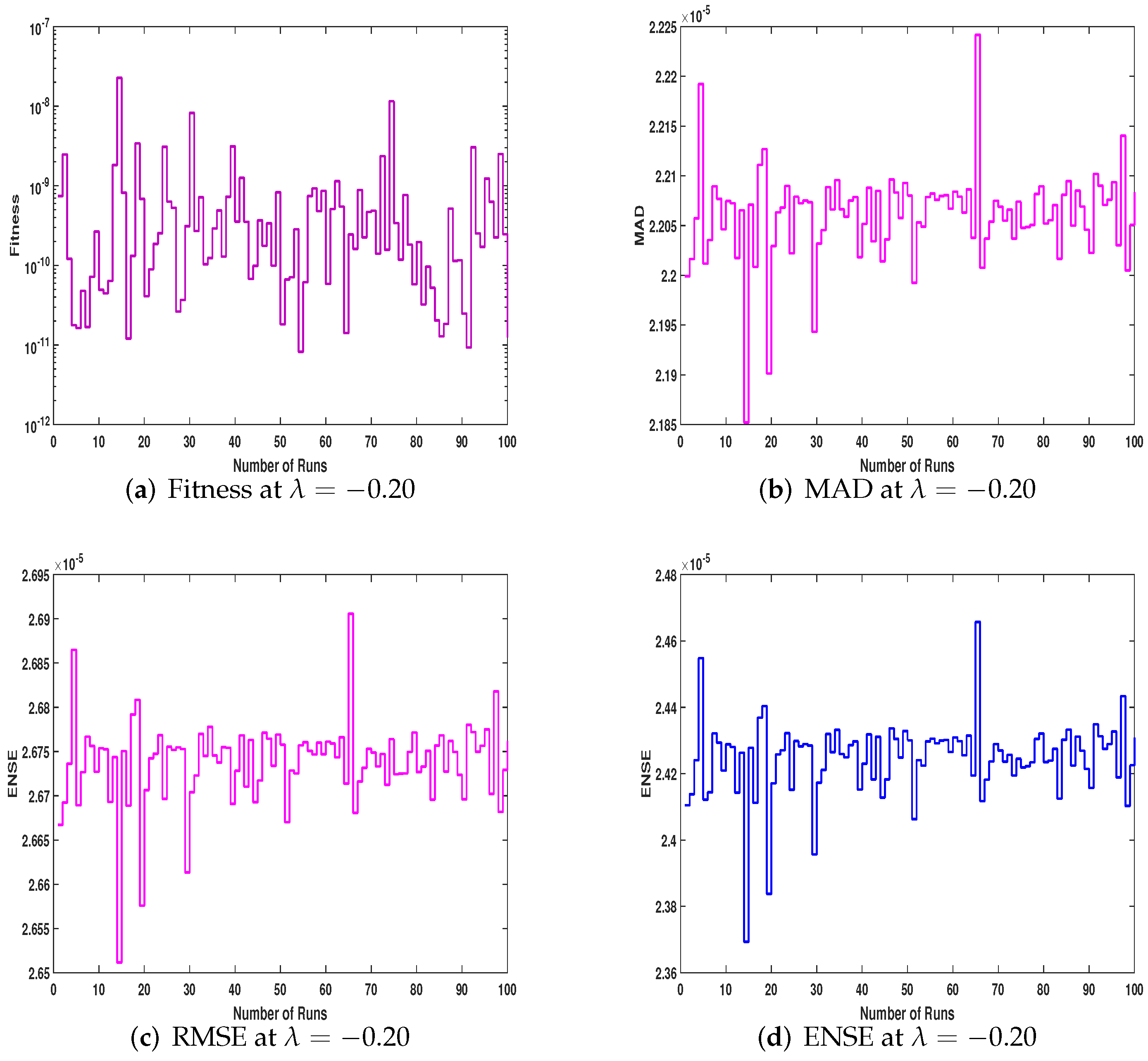
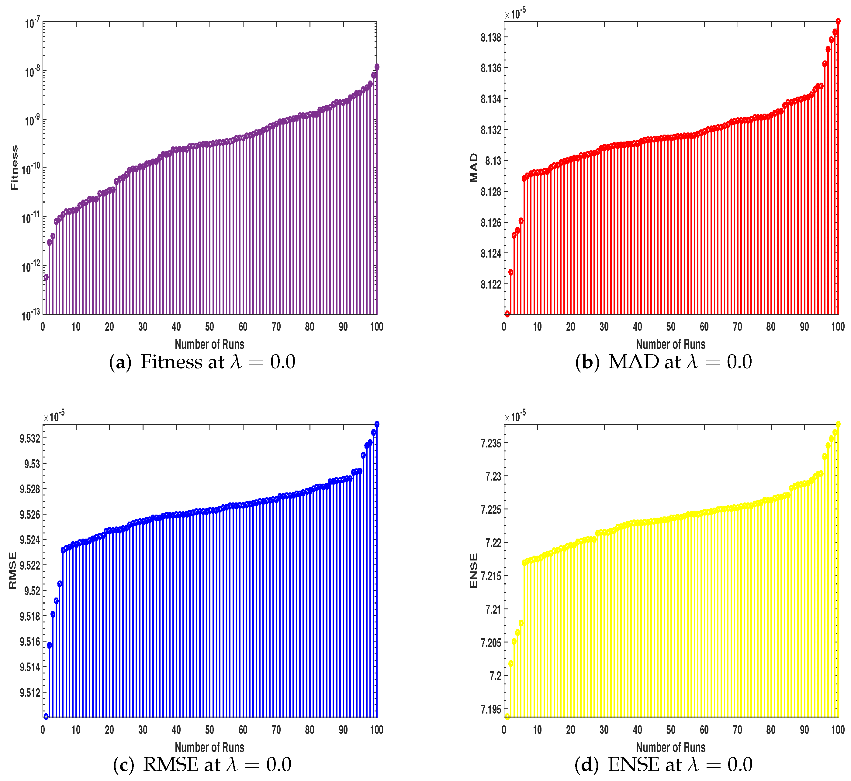
4.3. Performance Evaluation of SCA-SQP-ANN Algorithm

For the evaluation of the performance of the SCA-SQP-ANN algorithm, many techniques are adopted, such as numerical comparison of solutions, evaluation by performance operators, and graphical evaluations. The solutions are validated by comparing graphically and numerically. The reference solutions and proposed numerical solutions are compared numerically in Table 1 and Table 2. For the collection of large data sets, the proposed procedure was executed 100 times, as fewer executions cannot verify the consistency of any algorithm. All 100 solutions were drawn using a Mesh graph to verify the consistency of SCA-SQP-ANN, given in Figure 8a–f. From the figures, it can observe that there are no jumps and worst solutions. All the solutions are smoothly drawn. So that, the suggested algorithm i.e., SCA-SQP-ANN is consistent.
The data collected by multiple runs were evaluated by performance matrices MAD, RMSE, and ENSE as defined in Section 3.3. All the data are plotted in Figure 9a–d, Figure 10a–d, and Figure 11a–d, along with fitness. In Figure 9a–d, a stem graph is used for unsorted data of fitness and performance operators; the data in Figure 10a–d are plotted with a stairs plot; in Figure 11, the data are sorted and plotted with a stem plot. In each figure, the values are about 10 5 for MAD, RMSE, and ENSE. The fitness values are between 10 5 10 13 for each case of velocity and magnetic parameter.
Furthermore, the values of MAD, RMSE, and ENSE are evaluated by statistical terms mean, standard deviation, and minimum. The values of these statistical terms are given in Table 3. The STD of Problem 1 id between 10 5 to 10 8 , the values of mean is also between 10 5 to 10 8 and minimum values are lies between 10 5 to 10 13 . The values of performance matrices and fitness are up to considerable marks.
Moreover, the fitness values are briefly illustrated by the convergence graph boxplot, given in Figure 12a,b. The boxplot explains five quartile values. The first mark shows the minimum value, the second mark shows the first quartile called Q1, the third mark shows the median value and fourth mark shows the third quartile called Q3 and the fifth mark shows the maximum value. The range from Q1 to Q3 is known as the inter quartile range (IQR). On the x-axis, the cases of velocity ratio are given and on y-axis, the log is taken to observe a small variation in fitness values. The range of fitness values is considerable.

5. Conclusions

This work discussed Falkner–Skan flow under the influence of Hall magnetic effect. The flow is over a dynamic symmetric wedge. The x-axis and the wedge are parallel. Ordinary differential equations model the flow. For the solution of the mathematical model of MHD Falkner–Skan boundary layer flow, a novel hybrid technique is designed based on global search technique SCA and local search technique SQP. The system is transformed into an optimization problem by developing a fitness function. The fitness function is designed based on unsupervised mean square errors. The means square errors are minimized by training weights of ANN. The best weights, weights with minimum errors, are considered for solutions of the FSBLS model. A number of tests were conducted to evaluate the performance of SCA-SQP-ANN. First, the proposed algorithm’s exploration, exploitation, local optima avoidance, and convergence were examined. To validate the solutions of the SCA-SQP-ANN algorithm, the solution of RK4 is used as a benchmark answer. The solutions are visually contrasted and are given in Table 1 and Table 2. The performance of SCA-SQP-ANN was observed and verified statistically and qualitatively using a number of performance indicators, including MAD, RMSE, ENSE, fitness of solutions, and best solution during optimization.
The effectiveness of the SCA-SQP-ANN algorithm is found to be reliable and consistent. In the future, it can be used to solve many other physical, chemical, and biological phenomena.

Author Contributions

Conceptualization, K.N., M.F.K., M.S., F.S.A. and G.L.; Formal analysis, K.N., M.F.K., M.S. and F.S.A.; Investigation, M.F.K., M.S., F.S.A. and G.L.; Methodology, K.N., M.F.K., M.S., F.S.A. and G.L.; Resources, F.S.A. and G.L.; Software, G.L.; Supervision, M.S.; Validation, K.N. and F.S.A.; Visualization, M.F.K. and G.L.; Writing–original draft, M.F.K.; Writing–review & editing, K.N., M.F.K., M.S., F.S.A. and G.L. All authors have read and agreed to the published version of the manuscript.

Funding

This research received funding support from the National Science, Research, and Innovation Fund (NSRF), Thailand.

Data Availability Statement

The data that support the findings of this study are available from the corresponding author upon reasonable request.

Acknowledgments

We would like to thank the referees for their valuable comments and helpful advice on our manuscript.

Conflicts of Interest

The authors declare no conflict of interest.

Abbreviations

The following abbreviations are used in this manuscript:
MINMinimum
MAXMaximum
STDStandard Deviation
BLFBoundary Layer Flow
IQRInter Quartile Range
SCASine–Cosine Algorithm
RMSERoot Mean Square Error
MADMean Absolute Deviation
ANNArtificial Neural Network
ENSEError in Nash–Sutcliffe Efficiency
RK4Runge–Kutta order four technique
SQPSequential Quadratic Programming
FS-HTMFalkner–Skan Heat Transfer Model

Appendix A

Solutions of all problems
Solutions of Problem 1
f c 1 ( η ) = 0.95451934267321 1 + e ( 1.38227991398708 η 3.41246444537430 ) + 0.29140705604400 1 + e ( 1.04290268851165 η 1.16584125040135 ) + 2.46075758739035 1 + e ( 1.30598996253714 η 1.64686367799313 ) + 1.72285206620454 1 + e ( 1.00743149544052 η + 0.40373208094877 ) + 1.52325996181440 1 + e ( 1.78201504626318 η 0.91788006564095 ) + 1.43051072566624 1 + e ( 0.04123665946416 η 2.23231899085786 ) + 3.83221835578673 1 + e ( 1.44629037919505 η 4.03117833828382 ) + 3.27790774265310 1 + e ( 2.41209402355583 η + 3.13378927875832 ) + 1.44383109630061 1 + e ( 0.63095262839996 η + 0.42503522136513 ) + 0.83377436495192 1 + e ( 0.51698064357124 η 0.92841692624979 )
θ c 1 ( η ) = 0.88048796102550 1 + e ( 0.70450613620051 η 0.89880479987698 ) + 0.99783666539746 1 + e ( 1.75296133574524 η + 0.73176962985480 ) + 0.80663922047375 1 + e ( 0.72937043524787 η 0.90308156589137 ) + 0.38228699074710 1 + e ( 0.99713049500746 η 0.64765841518093 ) + 0.85613689118940 1 + e ( 0.69625201750333 η 0.88813893117092 ) + 0.74543970576107 1 + e ( 0.75480935551765 η 0.89071049845401 ) + 0.67496562826914 1 + e ( 0.81951189704188 η 0.73649711942888 ) + 0.78224464381023 1 + e ( 0.70013742967296 η 0.54969613341636 ) + 0.77028952689972 1 + e ( 1.52964158987318 η + 0.50423711612537 ) + 0.89517540637731 1 + e ( 1.90923528146009 η 2.27148358804469 )
f C 2 ( η ) = 0.92564213213197 1 + e ( 0.85899126561237 η 2.76046407649979 ) + 3.67695229438456 1 + e ( 1.40032470606699 η 3.83562682188711 ) + 2.66996813997215 1 + e ( 1.16606295656544 η 1.44209565379599 ) + 0.54560736013291 1 + e ( 0.76673389291917 η + 1.12912231039017 ) + 0.97752678467114 1 + e ( 1.05245116894721 η 0.67563481760404 ) + 0.36970475561443 1 + e ( 0.75416267446848 η + 1.16396516667487 ) + 4.75814360509627 1 + e ( 2.34304810139773 η 4.48889859425853 ) + 0.83065143159330 1 + e ( 1.21155430248592 η + 1.77176699057118 ) + 0.31965279961377 1 + e ( 0.35540745624133 η 0.51820670705212 ) + 1.57055412370019 1 + e ( 1.64313926997467 η 1.62297944498750 )
θ C 2 ( η ) = 0.81602284017935 1 + e ( 1.52399923295907 η 0.52508707631892 ) + 0.09009111128538 1 + e ( 0.91618036883607 η 0.24332210047278 ) + 1.21842773140496 1 + e ( 1.07844985009604 η 1.40092927066656 ) + 1.25566984776036 1 + e ( 1.66526421600737 η + 2.04421902349763 ) + 1.04673657369995 1 + e ( 0.32657268249953 η + 0.00860690369399 ) + 0.80610508998041 1 + e ( 0.74939370952166 η 0.00931395563917 ) + 1.40812482415235 1 + e ( 1.04717788747205 η 1.78848208661572 ) + 0.18013146077520 1 + e ( 1.24191289453316 η + 0.62443490366353 ) + 0.59745324846951 1 + e ( 1.01045132602252 η + 0.05089852847812 ) + 0.29548802891017 1 + e ( 1.63132586970201 η + 0.94128945051801 )
f C 3 ( η ) = 0.87484874581330 1 + e ( 0.82823748420746 η + 3.69377037484144 ) + 1.66504017852503 1 + e ( 1.01535213156728 η 0.32000006933361 ) + 0.88537393260607 1 + e ( 0.84569556514592 η + 0.24697171502457 ) + 5.15217815170286 1 + e ( 1.05249961874865 η 3.50239171005170 ) + 0.40850477299780 1 + e ( 0.43829008223205 η 0.01373991584687 ) + 5.74630105518434 1 + e ( 1.70917368300791 η 3.19278203271889 ) + 1.31893333273638 1 + e ( 0.77762703835820 η 0.74727179942460 ) + 1.91254034190604 1 + e ( 1.05947587109395 η 1.37210307688880 ) + 0.19087005385771 1 + e ( 0.17356079246086 η 1.04490304669672 ) + 0.52837327500167 1 + e ( 1.65541203008127 η + 0.98453500590823 )
θ C 3 ( η ) = 0.55532223398039 1 + e ( 0.83742641858779 η 0.99639581629085 ) + 0.02732616540500 1 + e ( 0.72982218487077 η + 0.75472883834036 ) + 0.86686851552658 1 + e ( 1.78695019990571 η + 2.05843122271539 ) + 0.71601093308008 1 + e ( 0.65212488631886 η + 0.60439416300282 ) + 0.83166937675384 1 + e ( 0.84606607395185 η 1.09576468208444 ) + 0.66486989239678 1 + e ( 0.91699773864743 η + 1.04871592250542 ) + 0.26183380239296 1 + e ( 0.22391052504993 η 1.00858347225341 ) + 0.68492062797319 1 + e ( 1.74332161712346 η + 0.72084550460754 ) + 0.82394856698054 1 + e ( 0.85728643436115 η 1.07955235064387 ) + 0.26521089998344 1 + e ( 0.15466745236089 η 1.02153681816394 )
f C 4 ( η ) = 0.98709426947608 1 + e ( 0.31806383666458 η + 1.12699099349894 ) + 2.21016354149007 1 + e ( 1.08534399431885 η 2.18411242521694 ) + 2.12102473989062 1 + e ( 0.85107439415758 η + 3.21190386921421 ) + 0.77846295420165 1 + e ( 0.24828212198387 η + 0.02718763571152 ) + 0.20862870286716 1 + e ( 0.61261326769017 η + 0.42959245241447 ) + 5.03711583139712 1 + e ( 0.79381848106399 η 3.87678156875451 ) + 5.04476624650189 1 + e ( 0.40671305670597 η 4.66892339710828 ) + 0.95898467184980 1 + e ( 1.15489780615814 η + 5.67637194885379 ) + 1.13551660764383 1 + e ( 1.27339833447433 η + 0.88028476719194 ) + 4.42122894670949 1 + e ( 1.48947540123632 η 2.82876797476339 )
θ C 4 ( η ) = 0.09126922914209 1 + e ( 0.06026554558989 η 0.21372589635568 ) + 0.75760330557859 1 + e ( 0.13927733501821 η + 0.86851022036354 ) + 1.91700627679286 1 + e ( 1.32995860172251 η + 1.25979424839109 ) + 0.64068070102756 1 + e ( 0.58265692132287 η + 0.33629432430303 ) + 0.23789044648334 1 + e ( 0.19966291666801 η 0.36130654139811 ) + 2.07248884526900 1 + e ( 1.15640992029826 η 2.27576617868925 ) + 1.27024653495002 1 + e ( 1.32718353700909 η + 0.14901825495048 ) + 0.41705682529251 1 + e ( 1.00578292108429 η 0.22357998521483 ) + 1.01994873563028 1 + e ( 0.75059971727698 η 0.67116931369726 ) + 1.23293719648139 1 + e ( 0.68533495762387 η + 0.82620187017164 )
Solution of Problem 2
f C 1 ( η ) = 0.66936751620390 1 + e ( 0.75565629115221 η + 0.38295493544875 ) + 5.88617908052277 1 + e ( 1.98434467080967 η 3.30747058797309 ) + 7.13103379179006 1 + e ( 1.04823976986383 η 3.62049405763613 ) + 0.60532478544146 1 + e ( 0.25527620832414 η + 0.14668580620218 ) + 0.63925291188960 1 + e ( 0.47447779154866 η 0.07437419464812 ) + 0.21809485534479 1 + e ( 0.13725372503562 η 3.18087068242422 ) + 0.66579088353691 1 + e ( 1.75662558414155 η + 0.97138001003240 ) + 3.11351987012573 1 + e ( 0.97594688053681 η 1.01513417830122 ) + 3.37785233896804 1 + e ( 0.15361976252350 η 0.78509241187643 ) + 0.25761739304668 1 + e ( 0.56971593310121 η 0.56770177159964 )
θ C 1 ( η ) = 0.80061337939581 1 + e ( 1.65312759629419 η 1.96526448363152 ) + 0.78421041224360 1 + e ( 0.06413981894150 η 0.29484964633448 ) + 0.85745171507242 1 + e ( 1.51312884508591 η + 0.73056995898463 ) + 0.47156839572230 1 + e ( 0.51659396244922 η + 0.43362710950894 ) + 0.75635562073559 1 + e ( 0.26885906458932 η + 0.19043202470473 ) + 0.87670421681094 1 + e ( 1.15643833448744 η + 0.36502674962507 ) + 1.25540742127178 1 + e ( 1.07581611166042 η 1.11757321041304 ) + 0.12709193627327 1 + e ( 0.73549633526512 η 0.09652260059985 ) + 1.02586818301978 1 + e ( 0.79423274307579 η + 0.60556385234739 ) + 0.63053864530985 1 + e ( 0.13775876277933 η 1.02327603969104 )
f C 2 ( η ) = 0.99960812942138 1 + e ( 1.00444696667649 η 1.03823389619077 ) + 3.16631909383033 1 + e ( 0.22433119326107 η + 0.48728510542688 ) + 3.91713760729317 1 + e ( 1.30024892587467 η + 4.07550503886324 ) + 0.42570478316415 1 + e ( 0.30862090306014 η + 1.75198107463726 ) + 2.87264906821485 1 + e ( 1.55902278707962 η 1.32360175991360 ) + 2.21323799878153 1 + e ( 2.41025146418473 η + 3.41243974008563 ) + 2.82320866719948 1 + e ( 0.08068917110829 η + 0.74331080530510 ) + 2.05740955760773 1 + e ( 2.76163858268829 η + 3.86089176361016 ) + 1.72391824004836 1 + e ( 0.36935278177074 η + 0.12320011944520 ) + 4.21387873232179 1 + e ( 0.36779870099361 η 0.10968159407608 )
θ C 2 ( η ) = 0.12485273498428 1 + e ( 0.87344869180262 η + 0.03507971866023 ) + 0.93242836504091 1 + e ( 0.78794478066500 η 0.15448467539335 ) + 0.94461488863257 1 + e ( 0.52463401429670 η 1.07093937797937 ) + 0.67470679070692 1 + e ( 0.23238564787645 η 0.99418685008286 ) + 0.69815790594142 1 + e ( 0.26261691602021 η + 0.25592895444716 ) + 0.42017348707822 1 + e ( 1.23072254048899 η + 0.10452242202885 ) + 1.11236282730140 1 + e ( 1.61782998411228 η 1.54855364744034 ) + 0.84226463358485 1 + e ( 0.67694744204958 η 0.28789610462582 ) + 1.11145928628483 1 + e ( 1.41016046438023 η 0.16897477751277 ) + 0.10142366106746 1 + e ( 0.95216641812913 η + 0.48154036530997 )
f C 3 ( η ) = 0.85431854570749 1 + e ( 4.71998988034300 η 4.42466826918314 ) + 1.56165514141287 1 + e ( 1.80598421611488 η 1.74702989154470 ) + 1.50260900909030 1 + e ( 0.03559757981764 η + 2.66752210488786 ) + 5.18142928752948 1 + e ( 0.35308337319279 η 1.63756650382908 ) + 3.86151823447005 1 + e ( 1.49152323742529 η + 4.78269718905032 ) + 1.66106371666509 1 + e ( 0.61749751659212 η 0.37768424528247 ) + 2.16131191516048 1 + e ( 2.36249938407956 η 2.40506589891327 ) + 1.93900283534854 1 + e ( 0.84217371906180 η 0.46008399577153 ) + 1.99982800536457 1 + e ( 0.08213781573709 η 1.32601750088665 ) + 0.76760447263116 1 + e ( 1.33585662839985 η 1.38411924835156 )
θ C 3 ( η ) = 1.80132409761900 1 + e ( 1.46771268740203 η 1.45338697859629 ) + 1.35126486660310 1 + e ( 1.60599868738721 η + 0.86023868892394 ) + 1.76799773001182 1 + e ( 2.19502442557322 η + 1.48364101454140 ) + 1.06643330418972 1 + e ( 2.59617531600647 η 1.35803014229627 ) + 0.37737455073983 1 + e ( 1.01854799825906 η 0.83019043410573 ) + 0.35586682292378 1 + e ( 0.35857654570536 η + 0.10716744630138 ) + 0.01077892078635 1 + e ( 0.01743725748302 η + 0.91577887836475 ) + 0.39227795506199 1 + e ( 0.45657396762793 η 0.16861635985110 ) + 0.96027241068141 1 + e ( 0.25436519981889 η 0.50621361144977 ) + 0.65127838506617 1 + e ( 1.85268486034116 η + 0.36802894725922 )
f C 4 ( η ) = 0.24355258720705 1 + e ( 2.56575596992252 η + 1.77015983008902 ) + 4.46118218152415 1 + e ( 1.34229584514296 η 3.96229331223104 ) + 0.61575702001402 1 + e ( 0.05966729894950 η + 0.01162384324709 ) + 0.15193191092399 1 + e ( 0.25620606429531 η 0.45149186324379 ) + 2.96393666743521 1 + e ( 0.64411902286253 η + 1.72146500162767 ) + 4.24300663650284 1 + e ( 3.51947267851711 η 3.19295884425309 ) + 3.25783397360283 1 + e ( 1.05582602911991 η 1.51362321963957 ) + 0.44267547357364 1 + e ( 4.47910000518847 η + 4.68205680297471 ) + 0.13390906893247 1 + e ( 3.13069950997241 η + 0.76068188950819 ) + 3.74434566855979 1 + e ( 6.45628039295814 η + 7.59604766601533 )
θ C 4 ( η ) = 1.31014768923695 1 + e ( 1.61739190289228 η 0.61326412446848 ) + 0.28009171576680 1 + e ( 0.20768730513024 η + 0.81745072096726 ) + 0.95161429163881 1 + e ( 3.32168183399147 η 0.91025009226237 ) + 2.93861765606446 1 + e ( 1.99051934648369 η + 0.30454557935905 ) + 1.01140988571728 1 + e ( 0.09343444847200 η + 0.85888349802653 ) + 0.48801599338675 1 + e ( 0.64645095962285 η 0.58822138381555 ) + 0.29617743828943 1 + e ( 0.42852842970091 η 0.01630817377277 ) + 1.60794416150155 1 + e ( 1.99238931383184 η 0.75872802707927 ) + 1.36123471188443 1 + e ( 1.80362642540768 η + 2.12974425287982 ) + 0.62257274717420 1 + e ( 0.73276217599783 η 0.22880679237690 )

References

  1. Falkneb, V.; Skan, S.W. LXXXV. Solutions of the boundary-layer equations. Lond. Edinb. Dublin Philos. Mag. J. Sci. 1931, 12, 865–896. [Google Scholar] [CrossRef]
  2. Bararnia, H.; Ghasemi, E.; Soleimani, S.; Ghotbi, A.R.; Ganji, D.D. Solution of the Falkner–Skan wedge flow by HPM–Pade method. Adv. Eng. Softw. 2012, 43, 44–52. [Google Scholar] [CrossRef]
  3. Howarth, L. On the solution of the laminar boundary layer equations. Proc. R. Soc. London. Ser.-Math. Phys. Sci. 1938, 164, 547–579. [Google Scholar] [CrossRef] [Green Version]
  4. Barania, H.; Haghparast, N.; Miansari, M.; Barari, A. Flow analysis for the Falkner–Sken wedge flow. Curr. Sci. 2012, 103, 169–177. [Google Scholar]
  5. Sayyed, S.; Singh, B.; Bano, N. Analytical solution of MHD slip flow past a constant wedge within a porous medium using DTM-Padé. Appl. Math. Comput. 2018, 321, 472–482. [Google Scholar] [CrossRef]
  6. Abbasbandy, S.; Hayat, T. Solution of the MHD Falkner-Skan flow by homotopy analysis method. Commun. Nonlinear Sci. Numer. Simul. 2009, 14, 3591–3598. [Google Scholar] [CrossRef]
  7. Abbas, Z.; Sajid, M.; Hayat, T. MHD boundary-layer flow of an upper-convected Maxwell fluid in a porous channel. Theor. Comput. Fluid Dyn. 2006, 20, 229–238. [Google Scholar] [CrossRef]
  8. Mukhopadhyay, S.; Layek, G.; Samad, S.A. Study of MHD boundary layer flow over a heated stretching sheet with variable viscosity. Int. J. Heat Mass Transf. 2005, 48, 4460–4466. [Google Scholar] [CrossRef]
  9. Khazayinejad, M.; Nourazar, S. On the effect of spatial fractional heat conduction in MHD boundary layer flow using Gr-Fe3O4–H2O hybrid nanofluid. Int. J. Therm. Sci. 2022, 172, 107265. [Google Scholar] [CrossRef]
  10. Anusha, T.; Mahesh, R.; Mahabaleshwar, U.S.; Laroze, D. An MHD Marangoni Boundary Layer Flow and Heat Transfer with Mass Transpiration and Radiation: An Analytical Study. Appl. Sci. 2022, 12, 7527. [Google Scholar] [CrossRef]
  11. Guo, Z.; Tian, X.; Wu, Z.; Yang, J.; Wang, Q. Heat transfer of granular flow around aligned tube bank in moving bed: Experimental study and theoretical prediction by thermal resistance model. Energy Convers. Manag. 2022, 257, 115435. [Google Scholar] [CrossRef]
  12. Shankar Goud, B.; Dharmendar Reddy, Y.; Mishra, S. Joule heating and thermal radiation impact on MHD boundary layer Nanofluid flow along an exponentially stretching surface with thermal stratified medium. Proc. Inst. Mech. Eng. Part J. Nanomater. Nanoeng. Nanosyst. 2022, 23977914221100961. [Google Scholar] [CrossRef]
  13. Anusha, T.; Mahabaleshwar, U.; Sheikhnejad, Y. An MHD of nanofluid flow over a porous stretching/shrinking plate with mass transpiration and Brinkman ratio. Transp. Porous Media 2022, 142, 333–352. [Google Scholar] [CrossRef]
  14. Elsaid, E.M.; Abdelwahed, M. MHD Boundary Layer Analysis of Hybrid Nanofluid over 3-D Sinusoidal Cylinder. Res. Sq. 2022. [Google Scholar] [CrossRef]
  15. Cui, W.; Li, X.; Li, X.; Si, T.; Lu, L.; Ma, T.; Wang, Q. Thermal performance of modified melamine foam/graphene/paraffin wax composite phase change materials for solar-thermal energy conversion and storage. J. Clean. Prod. 2022, 367, 133031. [Google Scholar] [CrossRef]
  16. Rai, P.; Mishra, U. Numerical Simulation of Boundary Layer Flow Over a Moving Plate in The Presence of Magnetic Field and Slip Conditions. J. Adv. Res. Fluid Mech. Therm. Sci. 2022, 95, 120–136. [Google Scholar]
  17. Yaseen, M.; Rawat, S.K.; Kumar, M. Falkner–Skan Problem for a Stretching or Shrinking Wedge With Nanoparticle Aggregation. J. Heat Transf. 2022, 144, 102501. [Google Scholar] [CrossRef]
  18. Garia, R.; Rawat, S.K.; Kumar, M.; Yaseen, M. Hybrid nanofluid flow over two different geometries with Cattaneo–Christov heat flux model and heat generation: A model with correlation coefficient and probable error. Chin. J. Phys. 2021, 74, 421–439. [Google Scholar] [CrossRef]
  19. Ali, L.; Ali, B.; Liu, X.; Ahmed, S.; Shah, M.A. Analysis of bio-convective MHD Blasius and Sakiadis flow with Cattaneo-Christov heat flux model and chemical reaction. Chin. J. Phys. 2022, 77, 1963–1975. [Google Scholar] [CrossRef]
  20. RamReddy, C.; Saran, H.L. Dual solutions and their stability analysis for inclined magnetohydrodynamics and Joule effects in Ti-alloy nanofluid: Flow separation. Proc. Inst. Mech. Eng. Part J. Process. Mech. Eng. 2022, 09544089221102404. [Google Scholar] [CrossRef]
  21. Siddique, I.; Nadeem, M.; Ali, R.; Jarad, F. Bioconvection of MHD Second-Grade Fluid Conveying Nanoparticles over an Exponentially Stretching Sheet: A Biofuel Applications. Arab. J. Sci. Eng. 2022, 47, 1–14.i. [Google Scholar] [CrossRef]
  22. Das, C.; Wang, G.; Payne, F. Some practical applications of magnetohydrodynamic pumping. Sens. Actuators A Phys. 2013, 201, 43–48. [Google Scholar] [CrossRef]
  23. Kudenatti, R.B.; Kirsur, S.R.; Achala, L.; Bujurke, N. Exact solution of two-dimensional MHD boundary layer flow over a semi-infinite flat plate. Commun. Nonlinear Sci. Numer. Simul. 2013, 18, 1151–1161. [Google Scholar] [CrossRef] [Green Version]
  24. Ishak, A.; Nazar, R.; Pop, I. MHD boundary-layer flow past a moving wedge. Magnetohydrodynamics 2009, 45, 103–110. [Google Scholar]
  25. Ali, B.; Hussain, S.; Naqvi, S.I.R.; Habib, D.; Abdal, S. Aligned magnetic and bioconvection effects on tangent hyperbolic nanofluid flow across faster/slower stretching wedge with activation energy: Finite element simulation. Int. J. Appl. Comput. Math. 2021, 7, 149. [Google Scholar] [CrossRef]
  26. Yacob, N.A.; Ishak, A.; Nazar, R.; Pop, I. Falkner–Skan problem for a static and moving wedge with prescribed surface heat flux in a nanofluid. Int. Commun. Heat Mass Transf. 2011, 38, 149–153. [Google Scholar] [CrossRef]
  27. Xia, C.; Zhu, Y.; Zhou, S.; Peng, H.; Feng, Y.; Zhou, W.; Shi, J.; Zhang, J. Simulation study on transient performance of a marine engine matched with high-pressure SCR system. Int. J. Engine Res. 2022, 14680874221084052. [Google Scholar] [CrossRef]
  28. Habib, D.; Salamat, N.; Abdal, S.H.S.; Ali, B. Numerical investigation for MHD Prandtl nanofluid transportation due to a moving wedge: Keller box approach. Int. Commun. Heat Mass Transf. 2022, 135, 106141. [Google Scholar] [CrossRef]
  29. Habib, D.; Salamat, N.; Ahsan, M.; Abdal, S.; Siddique, I.; Ali, B. Significance of bioconvection and mass transpiration for MHD micropolar Maxwell nanofluid flow over an extending sheet. Waves Random Complex Media 2022, 1–15. [Google Scholar] [CrossRef]
  30. Guo, Z.; Yang, J.; Tan, Z.; Tian, X.; Wang, Q. Numerical study on gravity-driven granular flow around tube out-wall: Effect of tube inclination on the heat transfer. Int. J. Heat Mass Transf. 2021, 174, 121296. [Google Scholar] [CrossRef]
  31. Marinca, V.; Herişanu, N. Application of optimal homotopy asymptotic method for solving nonlinear equations arising in heat transfer. Int. Commun. Heat Mass Transf. 2008, 35, 710–715. [Google Scholar] [CrossRef]
  32. Ali, B.; Hussain, S.; Nie, Y.; Rehman, A.U.; Khalid, M. Buoyancy effetcs on falknerskan flow of a Maxwell nanofluid fluid with activation energy past a wedge: Finite element approach. Chin. J. Phys. 2020, 68, 368–380. [Google Scholar] [CrossRef]
  33. Bejan, A. Second-law analysis in heat transfer and thermal design. In Advances in Heat Transfer; Elsevier: Amsterdam, The Netherlands, 1982; Volume 15, pp. 1–58. [Google Scholar]
  34. Makinde, O. Entropy analysis for MHD boundary layer flow and heat transfer over a flat plate with a convective surface boundary condition. Int. J. Exergy 2012, 10, 142–154. [Google Scholar] [CrossRef]
  35. Butt, A.S.; Ali, A. Entropy generation in MHD flow over a permeable stretching sheet embedded in a porous medium in the presence of viscous dissipation. Int. J. Exergy 2013, 13, 85–101. [Google Scholar] [CrossRef]
  36. Dehsara, M.; Dalir, N.; Nobari, M.R.H. Numerical analysis of entropy generation in nanofluid flow over a transparent plate in porous medium in presence of solar radiation, viscous dissipation and variable magnetic field. J. Mech. Sci. Technol. 2014, 28, 1819–1831. [Google Scholar] [CrossRef]
  37. Yazdi, M.H.; Abdullah, S.; Hashim, I.; Sopian, K. Entropy generation analysis of open parallel microchannels embedded within a permeable continuous moving surface: Application to magnetohydrodynamics (MHD). Entropy 2011, 14, 1–23. [Google Scholar] [CrossRef]
  38. Khan, M.F.; Sulaiman, M.; Romero, C.A.T.; Alkhathlan, A. Falkner–Skan Flow with Stream-Wise Pressure Gradient and Transfer of Mass over a Dynamic Wall. Entropy 2021, 23, 1448. [Google Scholar] [CrossRef]
  39. Fawad Khan, M.; Bonyah, E.; Alshammari, F.S.; Ghufran, S.M.; Sulaiman, M. Modelling and Analysis of Virotherapy of Cancer Using an Efficient Hybrid Soft Computing Procedure. Complexity 2022, 2022, 9660746. [Google Scholar] [CrossRef]
  40. Cui, W.; Si, T.; Li, X.; Li, X.; Lu, L.; Ma, T.; Wang, Q. Heat transfer analysis of phase change material composited with metal foam-fin hybrid structure in inclination container by numerical simulation and artificial neural network. Energy Rep. 2022, 8, 10203–10218. [Google Scholar] [CrossRef]
  41. Huang, K.; Su, B.; Li, T.; Ke, H.; Lin, M.; Wang, Q. Numerical simulation of the mixing behaviour of hot and cold fluids in the rectangular T-junction with/without an impeller. Appl. Therm. Eng. 2022, 204, 117942. [Google Scholar] [CrossRef]
  42. Khan, M.F.; Sulaiman, M.; Romero, C.A.T.; Alshammari, F.S. A Quantitative Study of Non-Linear Convective Heat Transfer Model by Novel Hybrid Heuristic Driven Neural Soft Computing. IEEE Access 2022, 10, 34133–34153. [Google Scholar] [CrossRef]
  43. Huang, W.; Jiang, T.; Zhang, X.; Khan, N.A.; Sulaiman, M. Analysis of beam-column designs by varying axial load with internal forces and bending rigidity using a new soft computing technique. Complexity 2021, 2021, 6639032. [Google Scholar] [CrossRef]
  44. Khan, M.F.; Sulaiman, M.; Tavera Romero, C.A.; Alkhathlan, A. A hybrid metaheuristic based on neurocomputing for analysis of unipolar electrohydrodynamic pump flow. Entropy 2021, 23, 1513. [Google Scholar] [CrossRef]
  45. Khan, N.A.; Sulaiman, M.; Kumam, P.; Aljohani, A.J. A new soft computing approach for studying the wire coating dynamics with Oldroyd 8-constant fluid. Phys. Fluids 2021, 33, 036117. [Google Scholar] [CrossRef]
  46. Wolpert, D.H.; Macready, W.G. No free lunch theorems for optimization. IEEE Trans. Evol. Comput. 1997, 1, 67–82. [Google Scholar] [CrossRef] [Green Version]
  47. Berrehal, H. Thermodynamics second law analysis for MHD boundary layer flow and heat transfer caused by a moving wedge. J. Mech. Sci. Technol. 2019, 33, 2949–2955. [Google Scholar] [CrossRef]
  48. Mirjalili, S. SCA: A sine cosine algorithm for solving optimization problems. Knowl.-Based Syst. 2016, 96, 120–133. [Google Scholar] [CrossRef]
  49. Mirjalili, S.M.; Mirjalili, S.Z.; Saremi, S.; Mirjalili, S. Sine cosine algorithm: Theory, literature review, and application in designing bend photonic crystal waveguides. In Nature-Inspired Optimizers; Springer: Berlin/Heidelberg, Germany, 2020; pp. 201–217. [Google Scholar]
  50. Zhao, M.; Wang, X.; Yu, J.; Bi, L.; Xiao, Y.; Zhang, J. Optimization of construction duration and schedule robustness based on hybrid grey wolf optimizer with sine cosine algorithm. Energies 2020, 13, 215. [Google Scholar] [CrossRef] [Green Version]
  51. Dasgupta, K.; Roy, P.K.; Mukherjee, V. Power flow based hydro-thermal-wind scheduling of hybrid power system using sine cosine algorithm. Electr. Power Syst. Res. 2020, 178, 106018. [Google Scholar] [CrossRef]
  52. Hekimoğlu, B. Sine-cosine algorithm-based optimization for automatic voltage regulator system. Trans. Inst. Meas. Control 2019, 41, 1761–1771. [Google Scholar] [CrossRef]
  53. Suid, M.; Tumari, M.M.; Ahmad, M. A modified sine cosine algorithm for improving wind plant energy production. Int. J. Electr. Eng. Comput. Sci. 2019, 16, 101–106. [Google Scholar]
  54. Qi, H.; Qiao, Y.B.; Ren, Y.T.; Shi, J.W.; Zhang, Z.Y.; Ruan, L.M. Application of the sequential quadratic programming algorithm for reconstructing the distribution of optical parameters based on the time-domain radiative transfer equation. Opt. Express 2016, 24, 24297–24312. [Google Scholar] [CrossRef] [PubMed]
  55. Johansen, T.A.; Fossen, T.I.; Berge, S.P. Constrained nonlinear control allocation with singularity avoidance using sequential quadratic programming. IEEE Trans. Control Syst. Technol. 2004, 12, 211–216. [Google Scholar] [CrossRef] [Green Version]
  56. Attia, A.F.; El Sehiemy, R.A.; Hasanien, H.M. Optimal power flow solution in power systems using a novel Sine-Cosine algorithm. Int. J. Electr. Power Energy Syst. 2018, 99, 331–343. [Google Scholar] [CrossRef]
  57. Sindhu, R.; Ngadiran, R.; Yacob, Y.M.; Zahri, N.A.H.; Hariharan, M. Sine–cosine algorithm for feature selection with elitism strategy and new updating mechanism. Neural Comput. Appl. 2017, 28, 2947–2958. [Google Scholar] [CrossRef]
  58. Mehmood, A.; Zameer, A.; Ling, S.H.; ur Rehman, A.; Raja, M.A.Z. Integrated computational intelligent paradigm for nonlinear electric circuit models using neural networks, genetic algorithms and sequential quadratic programming. Neural Comput. Appl. 2020, 32, 10337–10357. [Google Scholar] [CrossRef]
Figure 1. The structure of the model in coordinate system.
Symmetry 14 02180 g001
Figure 2. Flow chart of optimization procedure.
Symmetry 14 02180 g002
Figure 3. Graphs of solution for Problem 1.
Symmetry 14 02180 g003
Figure 4. 3D bar graphs of weights trained by ANN.
Symmetry 14 02180 g004
Figure 5. Graphs of solution for Problem 2.
Symmetry 14 02180 g005
Figure 6. 3D bar graphs of weights trained by ANN.
Symmetry 14 02180 g006
Figure 7. Graphs of velocity and temperature profile for β = 0.1 , 1 , 2 , 4 .
Symmetry 14 02180 g007
Figure 8. Graphs of solution for Problem 1.
Symmetry 14 02180 g008
Figure 9. Evaluation by performance operators for λ = 0.35 .
Symmetry 14 02180 g009
Figure 10. Evaluation by performance operators for λ = 0.20 .
Symmetry 14 02180 g010
Figure 11. Evaluation by performance operators for λ = 0.0 .
Symmetry 14 02180 g011
Figure 12. Fitness evaluation for different values of λ and M.
Symmetry 14 02180 g012
Table 1. Problem 1: Numerical comparison of solution, f ( η ) , P r = 0.72 , B r = 0.1 , M = 1.0 , β = 0.4 .
Inputs ( η ) λ = 0.35 λ = 0.20 λ = 0 λ = 0.3
SCA-SQP-ANNRK4SCA-SQP-ANNRK4SCA-SQP-ANNRK4SCA-SQP-ANNRK4
0−4.25 × 10 6 044.57 × 10 6 0−8.36 × 10 6 0−1.10 × 10 6 0
0.1−0.027234253−0.027406741−0.012918254−0.0130673220.0060934180.0057790.0344702520.034387
0.2−0.039237642−0.039865281−0.011986216−0.0125309160.0240704820.0229160.0775968410.077297
0.3−0.036469018−0.0377288540.0023112340.0012182630.0534376430.0511030.1289499120.128355
0.4−0.019367556−0.0213490230.0295045240.027788310.0937171710.0900260.1881045960.187176
0.50.0116375670.0089202050.0691321580.0667835870.1444372470.1393570.2546406930.253379
0.60.056123020.0527191060.1207384290.1178027930.2051313120.1987520.3281439670.326577
0.70.1136689030.1096797340.1838717150.1804378290.2753383470.2678510.4082079060.406385
0.80.1838576950.1794242940.2580839210.2542735260.3546039450.3462760.4944357410.492423
0.90.2662739380.2615644130.3429311910.3388882370.4424819080.4336330.586442620.584314
10.360504020.3557013320.4379753230.4338552150.5385361210.5295130.683857820.681691
Table 2. Problem 1: Numerical comparison of solution, θ ( η ) , P r = 0.72 , B r = 0.1 , M = 1.0 , β = 0.4 .
Inputs λ = 0.35 λ = 0.20 λ = 0 λ = 0.30
SCA-SQP-ANNRK4SCA-SQP-ANNRK4SCA-SQP-ANNRK4SCA-SQP-ANNRK4
01.00000181211.00000022510.99999853110.9999996991
0.10.908604090.9085626190.9055214840.9054952250.9016770080.8967074760.8965440030.896546217
0.20.8147138720.8147154470.8090446650.8090573770.8019961010.7934649360.7926022730.792627911
0.30.7183801520.7184732990.710704950.7107935390.7011983140.6903994110.6885699230.688629628
0.40.6197440770.6199461890.61072610.6109023980.5996054590.587718950.5848976310.584992563
0.50.5190448840.5193455170.509422610.5096764030.4976159330.4857080880.4820828310.482205966
0.60.416622930.4169883160.40719870.4075014260.3956983860.3847214170.380658580.380796345
0.70.3129202950.3132987170.3045442320.304853350.2943825930.2851748210.2811803680.281314622
0.80.2084786610.2088055750.2020273870.2022909180.194247940.1875342370.1842114760.184321615
0.90.1039330.104135380.1002836130.1004443760.0959093950.0923018410.090307460.090372365
1−1.30 × 10 6 01.51 × 10 7 03.57 × 10 7 03.74 × 10 7 0
Table 3. Statistical evaluation of performance operators.
OperatorSTDMEANMINSTDMEANMINSTDMEANMIN
MAD5.29 × 10 06 2.56 × 10 05 2.54 × 10 05 4.59 × 10 06 2.21 × 10 05 2.19 × 10 05 3.74 × 10 06 4.79 × 10 05 4.78 × 10 05
RMSE5.32 × 10 08 3.10 × 10 05 3.08 × 10 05 4.71 × 10 08 2.67 × 10 05 2.65 × 10 05 3.80 × 10 08 5.82 × 10 05 5.81 × 10 05
ENSE1.98 × 10 07 4.35 × 10 05 4.27 × 10 05 1.15 × 10 07 2.42 × 10 05 2.37 × 10 05 1.43 × 10 07 8.29 × 10 05 8.23 × 10 05
FITNESS2.10 × 10 07 2.10 × 10 07 5.04 × 10 12 2.68 × 10 07 9.02 × 10 08 8.23 × 10 12 1.67 × 10 07 9.16 × 10 08 5.81 × 10 13
Publisher’s Note: MDPI stays neutral with regard to jurisdictional claims in published maps and institutional affiliations.

