

Antifragile Control Systems: The Case of an Anti-Symmetric Network Model of the Tumor-Immune-Drug Interactions


Abstract
1. Introduction
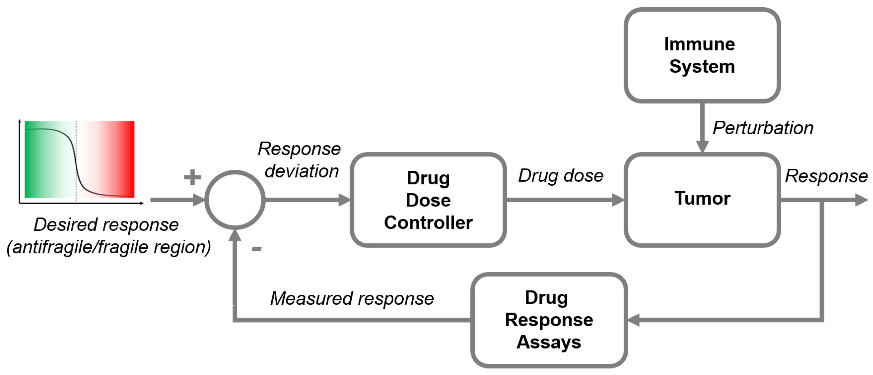
The Need for Control in Cancer Therapy
2. Materials and Methods
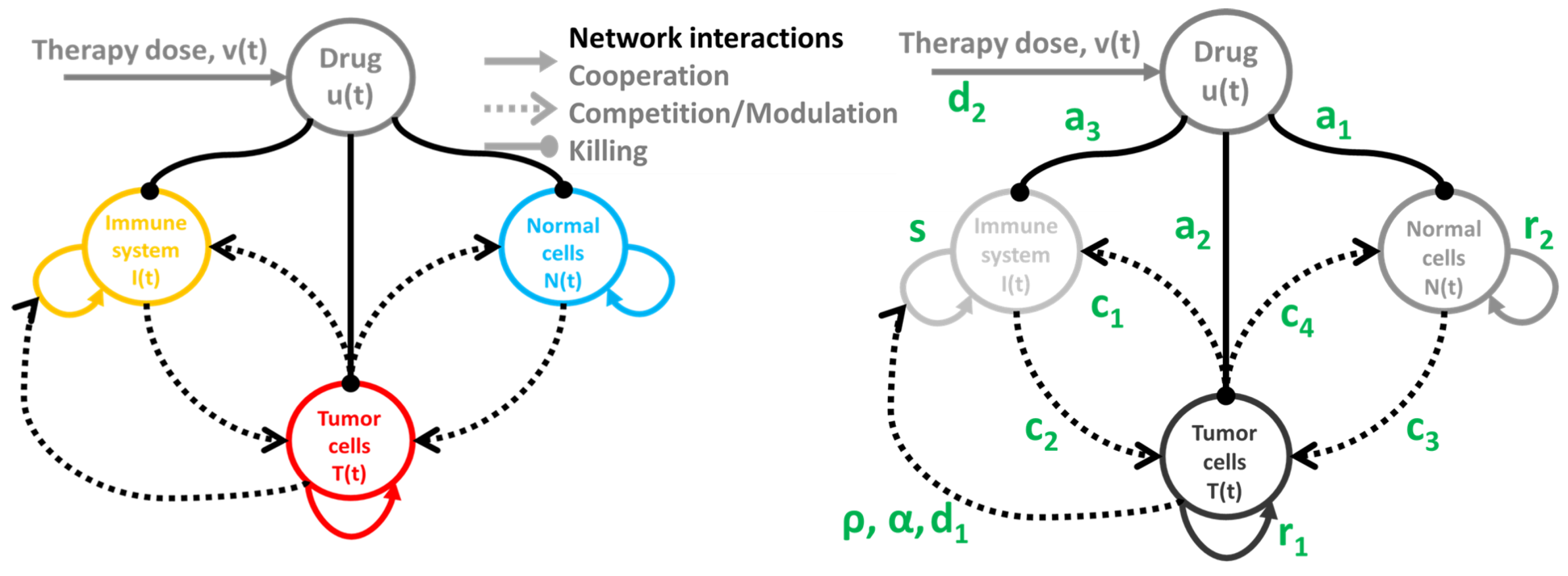
2.1. Tumor-Immune-Drug Network Model
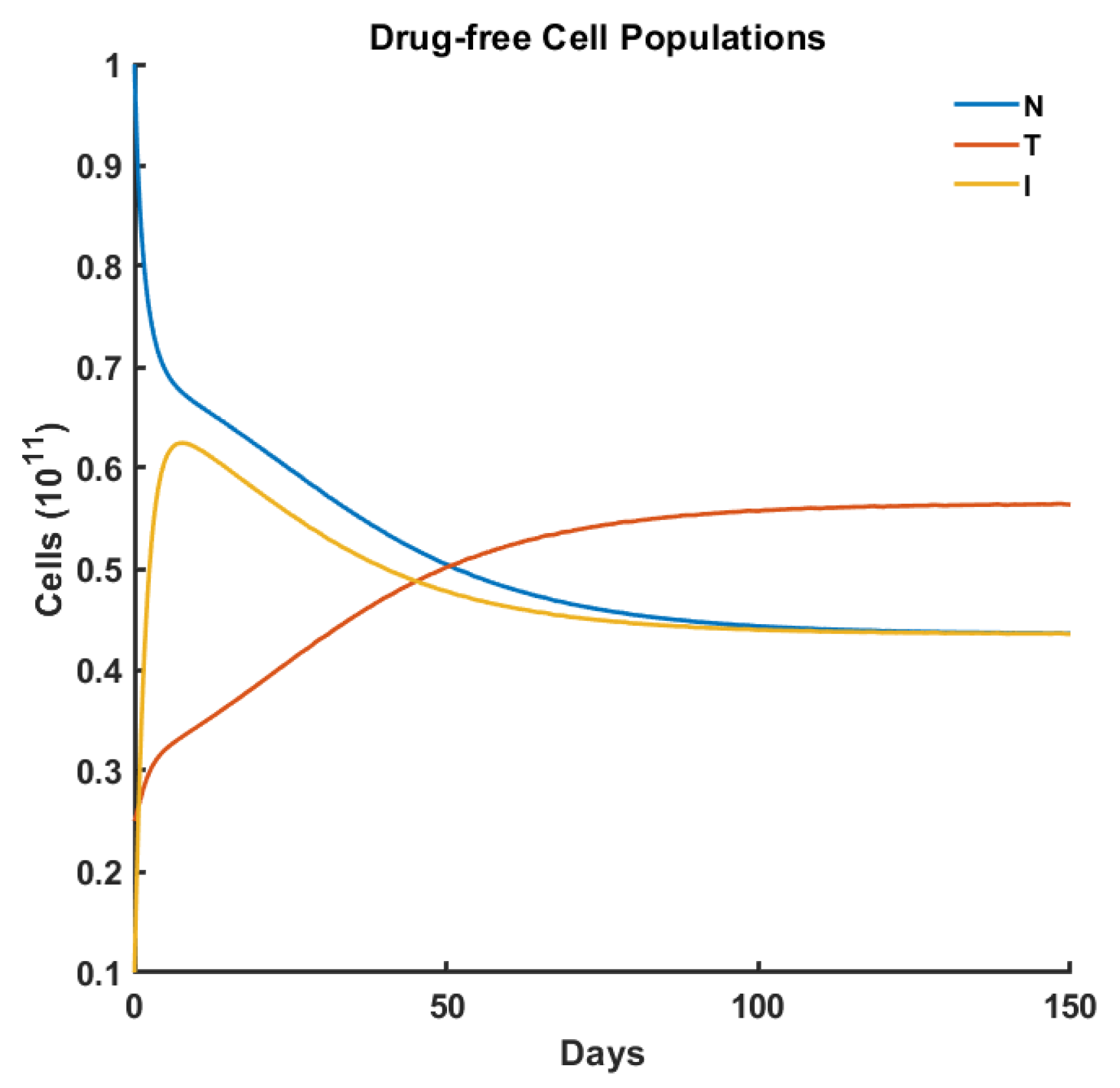
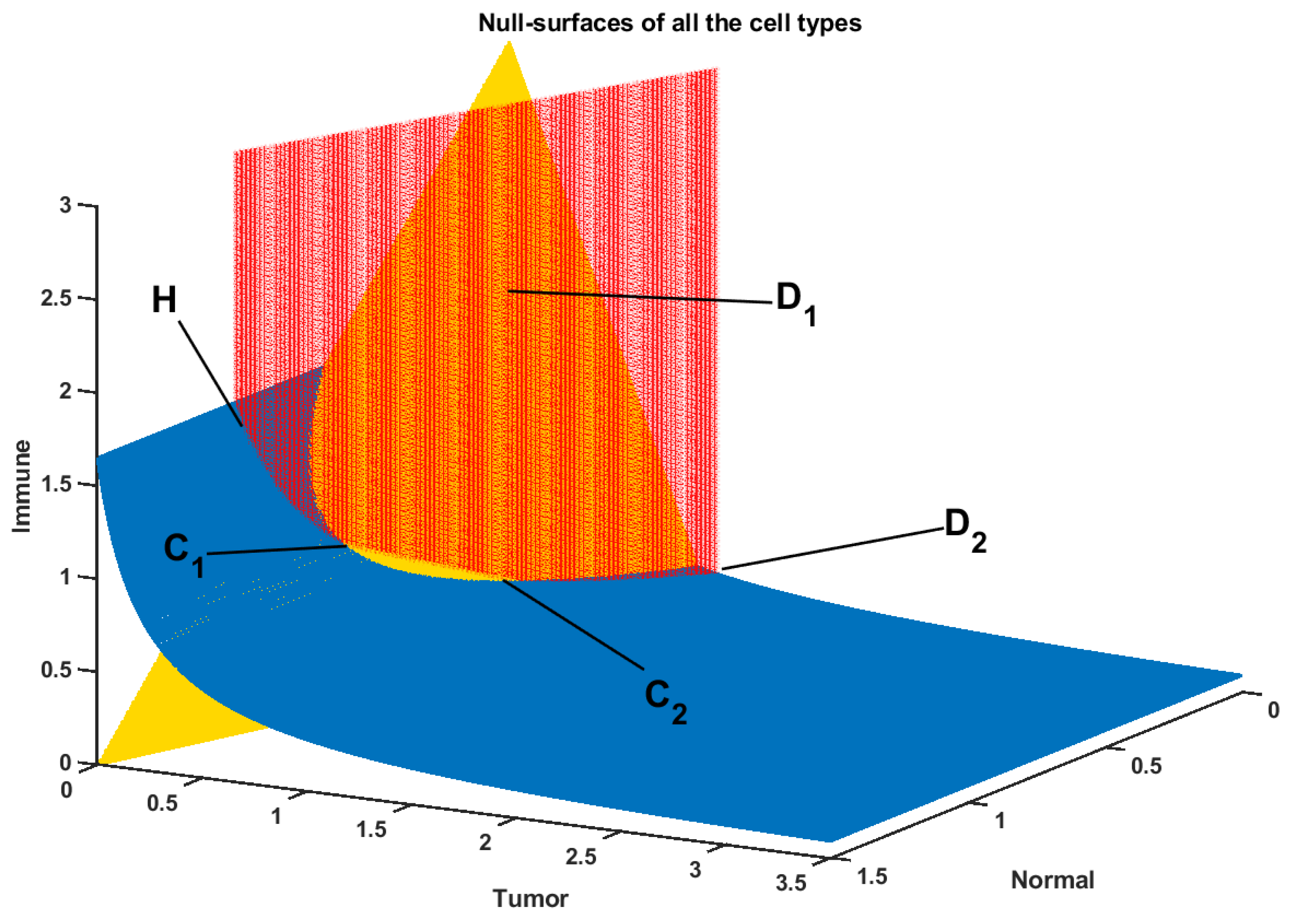
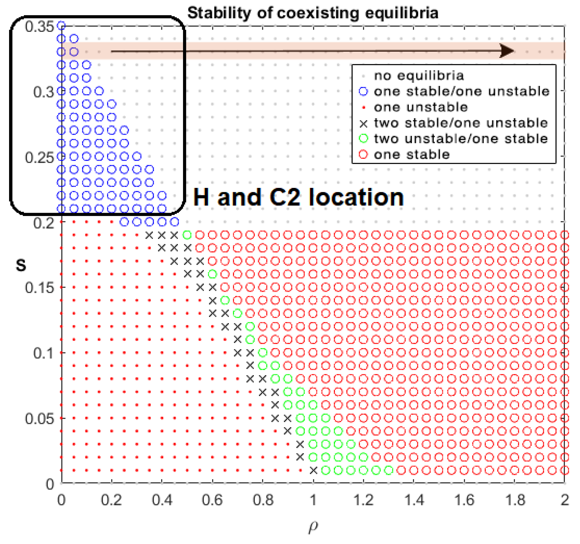
Drug-Free Evolution
2.2. Antifragile Control
2.2.1. Preliminaries
2.2.2. Formalism
Dynamical Systems on Manifolds
Control Error Function
Parallel Transport Map
2.2.3. Control Synthesis
Redundant Overcompensation
Stucture Variability
- the motion equation of the sliding mode, as nicely framed in Slotine et al. [32], can be designed linear and homogeneous, despite that the tumor-immune-drug model is governed by nonlinear equations,
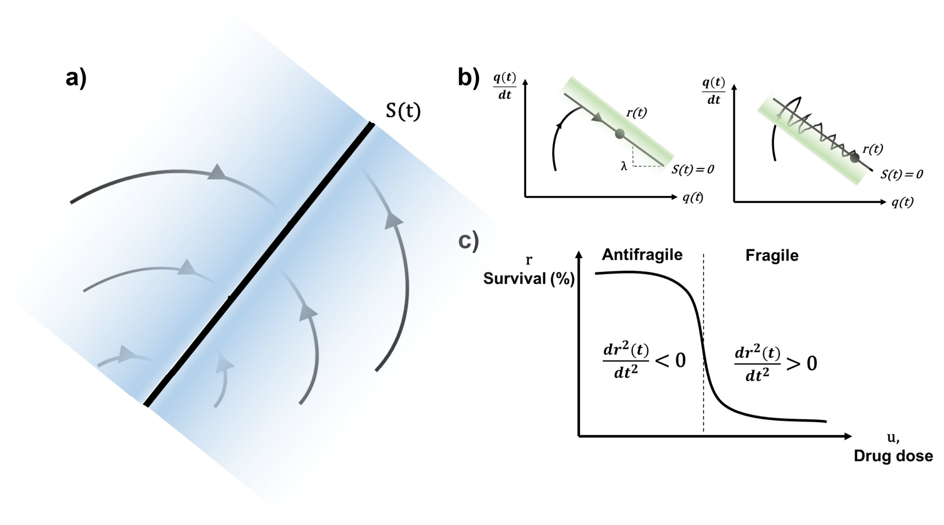
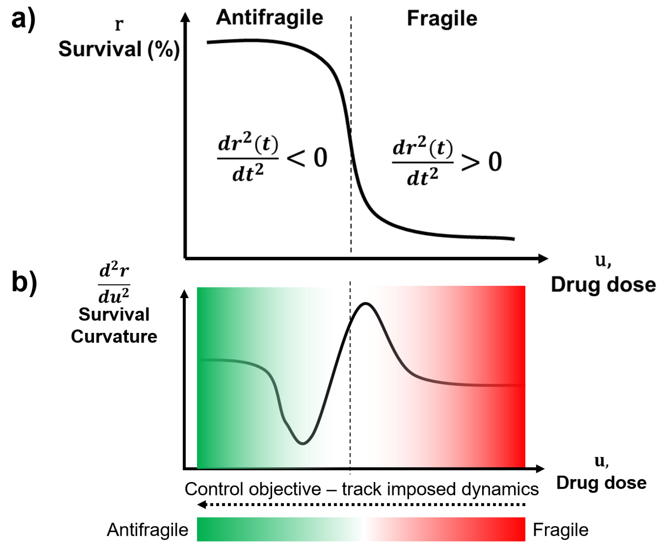
- the sliding surface does not depend on the process dynamics, but it is determined by parameters selected by the designer, as suggested in deCarlo et al. [33], i.e., desired trajectory of the system in the antifragile region of the drug dose–response curve (e.g., Hill function),
- once the sliding motion occurs (i.e., the system dynamics are on the surface), the system has invariant properties which make the motion independent of certain system parameter variations, uncertainty, and disturbances, as described in the famous work of Utkin [34]. Hence, the system performance can be completely determined by the dynamics of the sliding manifold.
Bounded High-Frequency Activity
2.3. State-of-the-Art Control Algorithms in Cancer Therapy
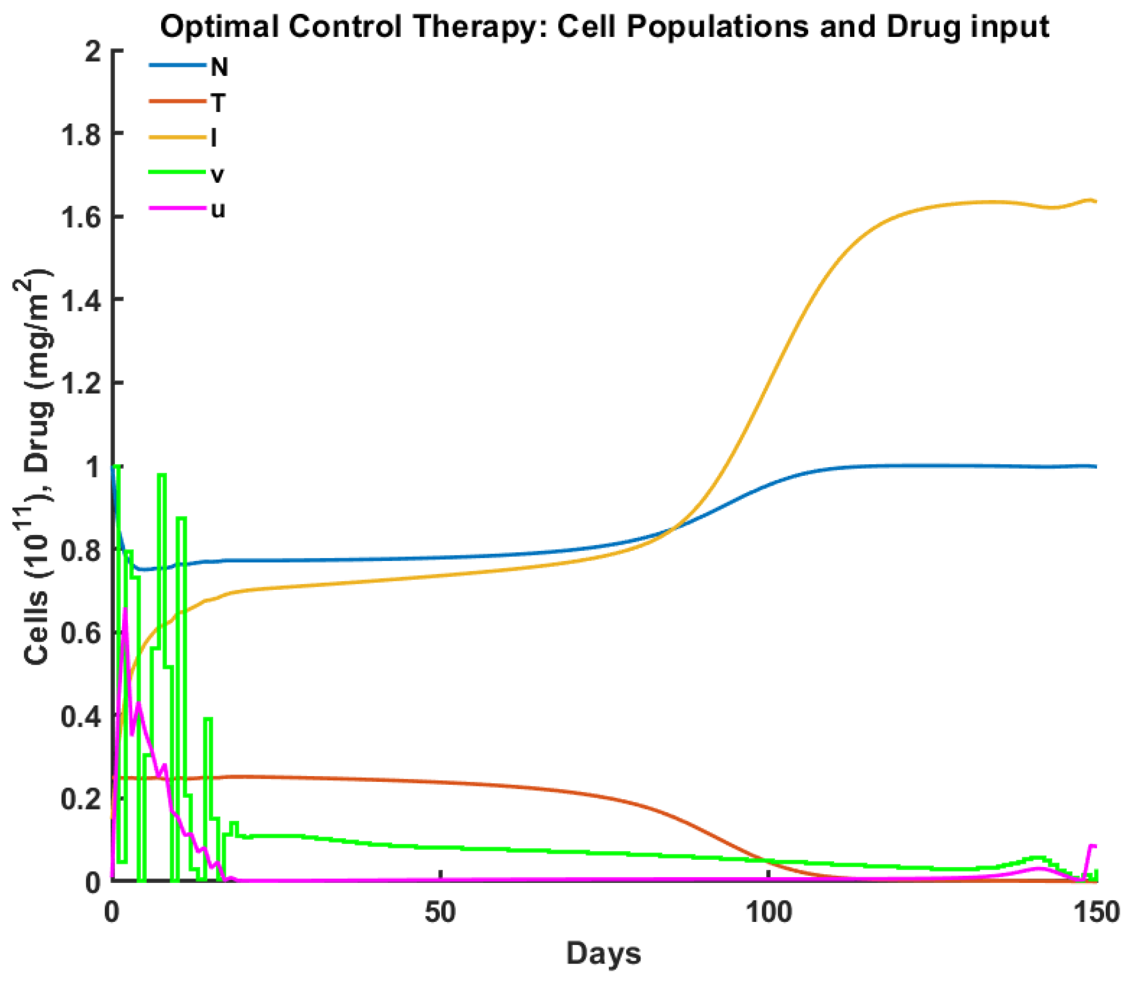
2.3.1. Optimal Control
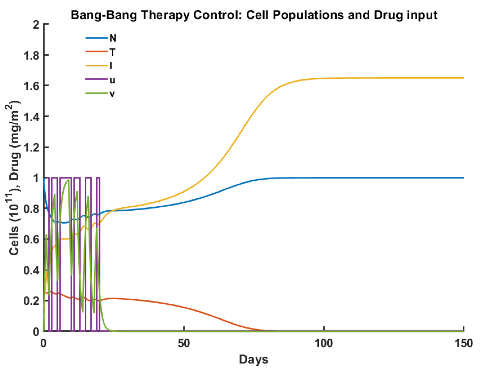
2.3.2. Robust Control
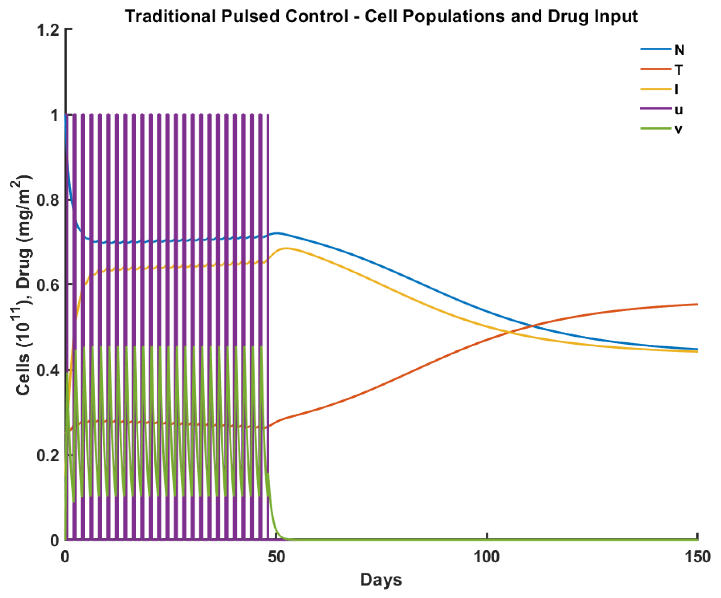
2.3.3. Pulsed Control
3. Experiments

| Model Parameter | Parameter (Initial) Value | Impact on Dynamics |
|---|---|---|
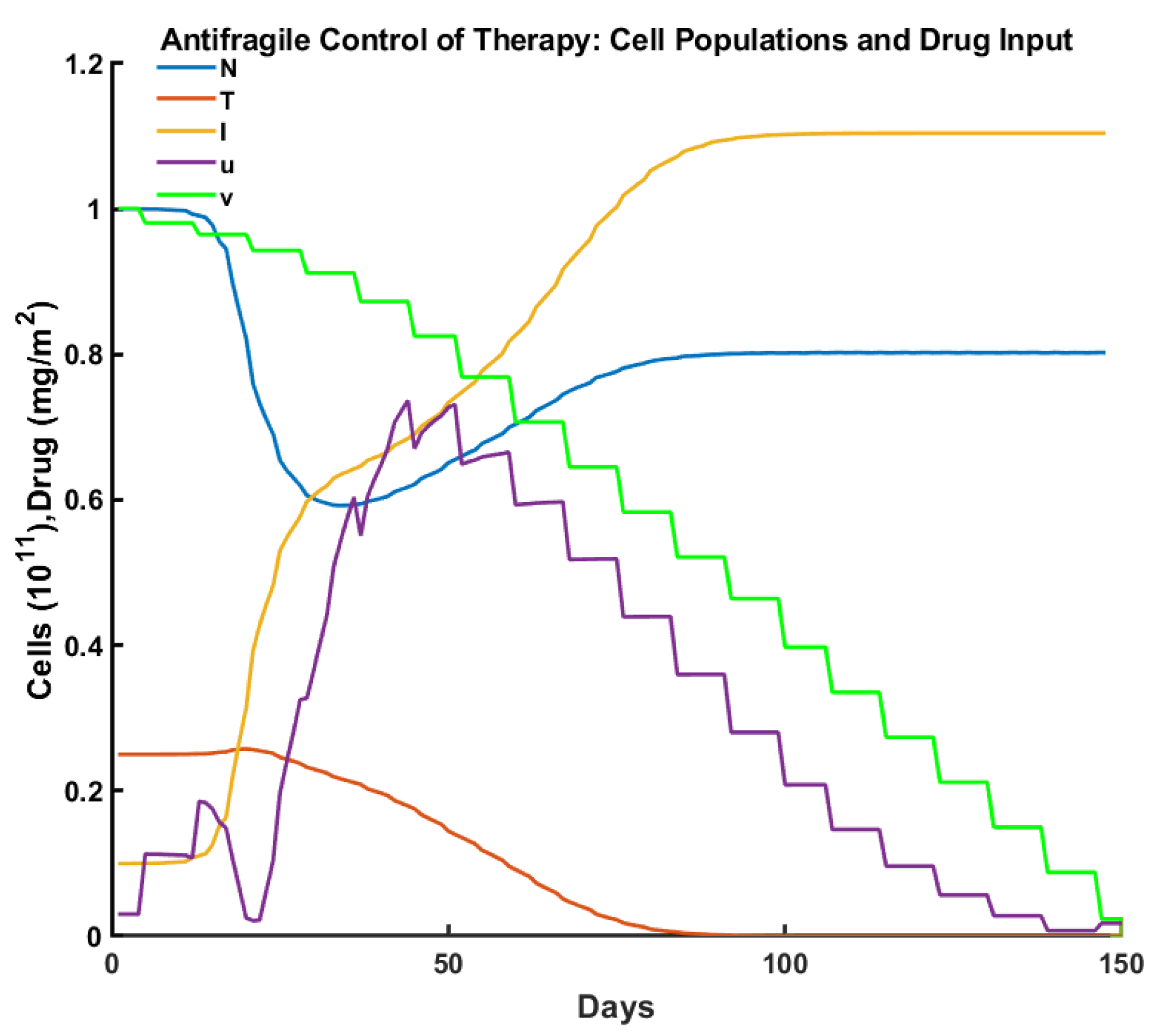
| Number of normal host cells N | 1.0 | Interacts with I and T w/wo u |
| Number of tumor cells T | 0.25 | Interacts with N and I w/wo u |
| Number of host immune cells I | 0.1 | Interacts with N and T w/wo u |
| Drug concentration at the tumor location u | 0.01 | induces cell kill by toxicity (normal+tumor) |
| Drug administration v | 0.0 | modulates the drug concentration at the tumor |
| Fraction normal cell kill | 0.2 | dose-related weight of normal cell kill (toxicity) |
| Fraction tumor cell kill | 0.3 | dose-related weight of tumor cell kill |
| Fraction immune cell kill | 0.1 | dose-related weight of immune cell kill |
| Tumor growth rate | 1.5 | typically |
| Normal cells growth rate | 1.0 | per capita growth |
| Carrying capacity of tumor cells | 1.0 | weights tumor cells self-excitation |
| Carrying capacity of normal cells | 1.0 | weights normal cells self-excitation |
| Tumor-immune competition factor | 1.0 | competition |
| Immune-tumor competition factor | 0.5 | modulation |
| Tumor-normal competition factor | 1.0 | competition |
| Normal-tumor competition factor | 1.0 | competition |
| Immune cells death rate | 0.2 | regulation through |
| Drug influx modulation | 1.0 | rate of change/decay of u |
| Immune threshold rate | 0.3 | related to the immune response curve |
| Immune response rate | 0.01–1.0 | immune-compromised to healthy |
4. Discussion
5. Conclusions
Author Contributions
Funding
Institutional Review Board Statement
Informed Consent Statement
Data Availability Statement
Conflicts of Interest
References
- Nia, H.T.; Munn, L.L.; Jain, R.K. Physical traits of cancer. Science 2020, 370, eaaz0868. [Google Scholar] [CrossRef]
- Schättler, H.; Ledzewicz, U. Optimal control for mathematical models of cancer therapies. In An Application of Geometric Methods; Springer: Berlin/Heidelberg, Germany, 2015. [Google Scholar]
- Kurz, D.; Sánchez, C.S.; Axenie, C. Data-driven Discovery of Mathematical and Physical Relations in Oncology Data using Human-understandable Machine Learning. Front. Artif. Intell. 2021, 4, 713690. [Google Scholar] [CrossRef] [PubMed]
- Belfo, J.P.; Lemos, J.M. Optimal Impulsive Control for Cancer Therapy; Springer: Berlin/Heidelberg, Germany, 2020. [Google Scholar]
- West, J.; Strobl, M.; Armagost, C.; Miles, R.; Marusyk, A.; Anderson, A.R. Antifragile therapy. bioRxiv 2020. [Google Scholar] [CrossRef]
- Kim, M.; Gillies, R.J.; Rejniak, K.A. Current advances in mathematical modeling of anti-cancer drug penetration into tumor tissues. Front. Oncol. 2013, 3, 278. [Google Scholar] [CrossRef] [PubMed]
- McDonald, E.; El-Deiry, W.S. Cell cycle control as a basis for cancer drug development. Int. J. Oncol. 2000, 16, 871–957. [Google Scholar] [CrossRef] [PubMed]
- Hu, X.; Jang, S.R.J. Dynamics of tumor–CD4+–cytokine–host cells interactions with treatments. Appl. Math. Comput. 2018, 321, 700–720. [Google Scholar] [CrossRef]
- Agur, Z.; Kheifetz, Y. Resonance and anti-resonance: From mathematical theory to clinical cancer treatment design. In Handbook of Cancer Models with Applications to Cancer Screening, Cancer Treatment and Risk Assessment; World Scientific: Singapore, 2005; Available online: http://dimat2.polito.it/~mcrtn/doc/lib/agur-kheifetz-resonance-2005.pdf (accessed on 31 August 2022).
- Agur, Z.; Kheifetz, Y. Optimizing Cancer Chemotherapy: From Mathematical Theories to Clinical Treatment. In New Challenges for Cancer Systems Biomedicine; Springer: Berlin/Heidelberg, Germany, 2012; pp. 285–299. [Google Scholar]
- Pillis, L.D.; Radunskaya, A. Modeling Immune-Mediated Tumor Growth and Treatment. In Mathematical Oncology 2013; Springer: Berlin/Heidelberg, Germany, 2014; pp. 199–235. [Google Scholar]
- De Pillis, L.G.; Radunskaya, A. The dynamics of an optimally controlled tumor model: A case study. Math. Comput. Model. 2003, 37, 1221–1244. [Google Scholar] [CrossRef]
- De Pillis, L.G.; Radunskaya, A. A mathematical tumor model with immune resistance and drug therapy: An optimal control approach. Comput. Math. Methods Med. 2001, 3, 79–100. [Google Scholar] [CrossRef]
- Kuznetsov, V.A.; Makalkin, I.A.; Taylor, M.A.; Perelson, A.S. Nonlinear dynamics of immunogenic tumors: Parameter estimation and global bifurcation analysis. Bull. Math. Biol. 1994, 56, 295–321. [Google Scholar] [CrossRef]
- Taleb, N.N. Antifragile: Things That Gain from Disorder; Random House: New York, NY, USA, 2012; Volume 3. [Google Scholar]
- Taleb, N.N. (Anti) fragility and convex responses in medicine. In Proceedings of the International Conference on Complex Systems, Cambridge, MA, USA, 22–27 July 2018; Springer: Berlin/Heidelberg, Germany, 2018; pp. 299–325. [Google Scholar]
- Goutelle, S.; Maurin, M.; Rougier, F.; Barbaut, X.; Bourguignon, L.; Ducher, M.; Maire, P. The Hill equation: A review of its capabilities in pharmacological modelling. Fundam. Clin. Pharmacol. 2008, 22, 633–648. [Google Scholar] [CrossRef]
- Gaffney, E.A. The application of mathematical modelling to aspects of adjuvant chemotherapy scheduling. J. Math. Biol. 2004, 48, 375–422. [Google Scholar] [CrossRef] [PubMed]
- Fedorinov, D.S.; Lyadov, V.K.; Sychev, D.A. Genotype-based chemotherapy for patients with gastrointestinal tumors: Focus on oxaliplatin, irinotecan, and fluoropyrimidines. Drug Metab. Pers. Ther. 2022, 37, 223–228. [Google Scholar] [CrossRef]
- Paraiso, K.H.; Smalley, K.S. Fibroblast-mediated drug resistance in cancer. Biochem. Pharmacol. 2013, 85, 1033–1041. [Google Scholar] [CrossRef] [PubMed]
- Bejenaru, A.; Udriste, C. Riemannian optimal control. arXiv 2012, arXiv:1203.3655. [Google Scholar]
- Lee, J.M. Riemannian Manifolds: An Introduction to Curvature; Springer Science & Business Media: Berlin/Heidelberg, Germany, 2006; Volume 176. [Google Scholar]
- Bloch, A.M. An introduction to aspects of geometric control theory. In Nonholonomic Mechanics and Control; Springer: Berlin/Heidelberg, Germany, 2015; pp. 199–233. [Google Scholar]
- Zou, L.; Wen, X.; Karimi, H.R.; Shi, Y. The identification of convex function on Riemannian manifold. Math. Probl. Eng. 2014, 2014, 899–908. [Google Scholar] [CrossRef]
- Bullo, F.; Murray, R.M.; Proportional Derivative (PD) Control on the Euclidean Group. Caltech Reports. 1995. Available online: https://authors.library.caltech.edu/28018/1/95-010.pdf (accessed on 31 August 2022).
- Bécigneul, G.; Ganea, O.E. Riemannian adaptive optimization methods. arXiv 2018, arXiv:1810.00760. [Google Scholar]
- Fiori, S. Manifold Calculus in System Theory and Control—Fundamentals and First-Order Systems. Symmetry 2021, 13, 2092. [Google Scholar] [CrossRef]
- Fiori, S.; Cervigni, I.; Ippoliti, M.; Menotta, C. Synchronization of dynamical systems on Riemannian manifolds by an extended PID-type control theory: Numerical evaluation. Discret. Contin. Dyn. Syst. B 2022, 27, 7373–7408. [Google Scholar] [CrossRef]
- Guo, Y.; Xu, B.; Zhang, R. Terminal sliding mode control of mems gyroscopes with finite-time learning. IEEE Trans. Neural Netw. Learn. Syst. 2020, 32, 4490–4498. [Google Scholar] [CrossRef]
- Colli, P.; Gilardi, G.; Marinoschi, G.; Rocca, E. Sliding mode control for a phase field system related to tumor growth. Appl. Math. Optim. 2019, 79, 647–670. [Google Scholar] [CrossRef]
- Ouyang, P.; Acob, J.; Pano, V. PD with sliding mode control for trajectory tracking. Robot. Comput.-Integr. Manuf. 2014, 30, 189–200. [Google Scholar] [CrossRef]
- Slotine, J.J.E.; Li, W. Applied Nonlinear Control; Prentice Hall: Englewood Cliffs, NJ, USA, 1991; Volume 199. [Google Scholar]
- DeCarlo, R.A.; Zak, S.H.; Matthews, G.P. Variable structure control of nonlinear multivariable systems: A tutorial. Proc. IEEE 1988, 76, 212–232. [Google Scholar] [CrossRef]
- Utkin, V. Variable structure systems with sliding modes. IEEE Trans. Autom. Control 1977, 22, 212–222. [Google Scholar] [CrossRef]
- Meyer, C.T.; Wooten, D.J.; Paudel, B.B.; Bauer, J.; Hardeman, K.N.; Westover, D.; Lovly, C.M.; Harris, L.A.; Tyson, D.R.; Quaranta, V. Quantifying drug combination synergy along potency and efficacy axes. Cell Syst. 2019, 8, 97–108. [Google Scholar] [CrossRef] [PubMed]
- Maithripala, D.S.; Berg, J.M. An intrinsic PID controller for mechanical systems on Lie groups. Automatica 2015, 54, 189–200. [Google Scholar] [CrossRef]
- Zhang, Z.; Sarlette, A.; Ling, Z. Integral control on Lie groups. Syst. Control Lett. 2015, 80, 9–15. [Google Scholar] [CrossRef]
- Lecca, P. Control Theory and Cancer Chemotherapy: How They Interact. Front. Bioeng. Biotechnol. 2021, 8, 621269. [Google Scholar] [CrossRef]
- Li, D.; Xu, W.; Guo, Y.; Xu, Y. Fluctuations induced extinction and stochastic resonance effect in a model of tumor growth with periodic treatment. Phys. Lett. A 2011, 375, 886–890. [Google Scholar] [CrossRef]
- Ren, H.P.; Yang, Y.; Baptista, M.S.; Grebogi, C. Tumour chemotherapy strategy based on impulse control theory. Philos. Trans. R. Soc. Math. Phys. Eng. Sci. 2017, 375, 20160221. [Google Scholar] [CrossRef]
- Swan, G.W. Role of optimal control theory in cancer chemotherapy. Math. Biosci. 1990, 101, 237–284. [Google Scholar] [CrossRef]
- Carrere, C. Optimization of an in vitro chemotherapy to avoid resistant tumours. J. Theor. Biol. 2017, 413, 24–33. [Google Scholar] [CrossRef] [PubMed]
- Irurzun-Arana, I.; Janda, A.; Ardanza-Trevijano, S.; Trocóniz, I.F. Optimal dynamic control approach in a multi-objective therapeutic scenario: Application to drug delivery in the treatment of prostate cancer. PLoS Comput. Biol. 2018, 14, 1–16. [Google Scholar] [CrossRef] [PubMed]
- Uthamacumaran, A. A review of dynamical systems approaches for the detection of chaotic attractors in cancer networks. Patterns 2021, 2, 100226. [Google Scholar] [CrossRef] [PubMed]
- Axenie, C.; Kurz, D. Chimera: Combining mechanistic models and machine learning for personalized chemotherapy and surgery sequencing in breast cancer. In Mathematical and Computational Oncology, Proceedings of the Second International Symposium, ISMCO 2020, San Diego, CA, USA, 8–10 October 2020; Springer: Berlin/Heidelberg, Germany, 2020; pp. 13–24. [Google Scholar]
- Wang, S. Optimal control for cancer chemotherapy under tumor heterogeneity. In Proceedings of the 2019 IEEE 58th Conference on Decision and Control (CDC), Nice, France, 11–13 December 2019; pp. 5936–5941. [Google Scholar]
- Ledzewicz, U.; Maurer, H.; Schättler, H. Bang-bang and singular controls in a mathematical model for combined anti-angiogenic and chemotherapy treatments. In Proceedings of the 48h IEEE Conference on Decision and Control (CDC) Held Jointly with 2009 28th Chinese Control Conference, Shanghai, China, 15–18 December 2009; pp. 2280–2285. [Google Scholar]
- Ledzewicz, U.; Schättler, H. Optimal bang-bang controls for a two-compartment model in cancer chemotherapy. J. Optim. Theory Appl. 2002, 114, 609–637. [Google Scholar] [CrossRef]
- Ledzewicz, U.; Schättler, H.; Gahrooi, M.R.; Dehkordi, S.M. On the MTD paradigm and optimal control for multi-drug cancer chemotherapy. Math. Biosci. Eng. 2013, 10, 803. [Google Scholar] [PubMed]
- Panetta, J.C. A mathematical model of periodically pulsed chemotherapy: Tumor recurrence and metastasis in a competitive environment. Bull. Math. Biol. 1996, 58, 425–447. [Google Scholar] [CrossRef]
- Kelly, M. An Introduction to Trajectory Optimization: How to do your own Direct Collocation. SIAM Rev. 2017, 59, 849–904. [Google Scholar] [CrossRef]
- Taleb, N.N.; Douady, R. Mathematical definition, mapping, and detection of (anti) fragility. Quant. Financ. 2013, 13, 1677–1689. [Google Scholar] [CrossRef]
- Axenie, C.; Kurz, D. Tumor characterization using unsupervised learning of mathematical relations within breast cancer data. In Proceedings of the International Conference on Artificial Neural Networks, Bratislava, Slovakia, 15–18 September 2020; Springer: Berlin/Heidelberg, Germany, 2020; pp. 838–849. [Google Scholar]
- Amin, D.N.; Sergina, N.; Ahuja, D.; McMahon, M.; Blair, J.A.; Wang, D.; Hann, B.; Koch, K.M.; Shokat, K.M.; Moasser, M.M. Resiliency and vulnerability in the HER2-HER3 tumorigenic driver. Sci. Transl. Med. 2010, 2, 16ra7. [Google Scholar] [CrossRef]
- Grommes, C.; Oxnard, G.R.; Kris, M.G.; Miller, V.A.; Pao, W.; Holodny, A.I.; Clarke, J.L.; Lassman, A.B. “Pulsatile” high-dose weekly erlotinib for CNS metastases from EGFR mutant non-small cell lung cancer. Neuro-oncology 2011, 13, 1364–1369. [Google Scholar] [CrossRef]
- Chmielecki, J.; Foo, J.; Oxnard, G.R.; Hutchinson, K.; Ohashi, K.; Somwar, R.; Wang, L.; Amato, K.R.; Arcila, M.; Sos, M.L.; et al. Optimization of dosing for EGFR-mutant non–small cell lung cancer with evolutionary cancer modeling. Sci. Transl. Med. 2011, 3, 90ra59. [Google Scholar] [CrossRef] [PubMed]
- Schöttle, J.; Chatterjee, S.; Volz, C.; Siobal, M.; Florin, A.; Rokitta, D.; Hinze, Y.; Dietlein, F.; Plenker, D.; König, K.; et al. Intermittent high-dose treatment with erlotinib enhances therapeutic efficacy in EGFR-mutant lung cancer. Oncotarget 2015, 6, 38458. [Google Scholar] [CrossRef] [PubMed][Green Version]


| Criteria/Control | Pulsed | Robust | Optimal | Antifragile |
|---|---|---|---|---|
| Time to tumor elimination (days) | 150+ | 68 | 100 | 65 |
| Max drug concentration (mg/L) | 0.455 | 0.987 | 0.659 | 0.736 |
| Total drug administered (mg/L) | 15.00 | 12.00 | 15.00 | 14.31 |
| Max tumor cells ( cells ) | 0.553 | 0.258 | 0.257 | 0.251 |
| Min normal cells ( cells) | 0.447 | 0.706 | 0.750 | 0.592 |
Publisher’s Note: MDPI stays neutral with regard to jurisdictional claims in published maps and institutional affiliations. |
© 2022 by the authors. Licensee MDPI, Basel, Switzerland. This article is an open access article distributed under the terms and conditions of the Creative Commons Attribution (CC BY) license (https://creativecommons.org/licenses/by/4.0/).
Share and Cite
Axenie, C.; Kurz, D.; Saveriano, M. Antifragile Control Systems: The Case of an Anti-Symmetric Network Model of the Tumor-Immune-Drug Interactions. Symmetry 2022, 14, 2034. https://doi.org/10.3390/sym14102034
Axenie C, Kurz D, Saveriano M. Antifragile Control Systems: The Case of an Anti-Symmetric Network Model of the Tumor-Immune-Drug Interactions. Symmetry. 2022; 14(10):2034. https://doi.org/10.3390/sym14102034
Chicago/Turabian StyleAxenie, Cristian, Daria Kurz, and Matteo Saveriano. 2022. "Antifragile Control Systems: The Case of an Anti-Symmetric Network Model of the Tumor-Immune-Drug Interactions" Symmetry 14, no. 10: 2034. https://doi.org/10.3390/sym14102034
APA StyleAxenie, C., Kurz, D., & Saveriano, M. (2022). Antifragile Control Systems: The Case of an Anti-Symmetric Network Model of the Tumor-Immune-Drug Interactions. Symmetry, 14(10), 2034. https://doi.org/10.3390/sym14102034