Motion of Particles around Time Conformal Dilaton Black Holes

Abstract

In this paper, the geodesic motion of neutral and test particles around the time conformal (TC) Dilaton black hole (BH) is investigated using the $e^{ϵg\left(t\right)}$ as the time conformal factor in which g(t) is an arbitrary function of time and $ϵ$ is a perturbation parameter. The function $g\left(t\right)$ leads to $\left(\frac{t}{a}\right)$ by utilizing the well-known approximate Noether symmetry (ANS). Furthermore, we discuss the effect of magnetic fields and find the location of stable and unstable orbits w. r. t time, graphically. After that, in the presence and absence of a magnetic field, we interrogate the crucial physical parameters such as effective potential $\left(U_{eff}\right)$, effective force $\left(F_{eff}\right)$ and escape velocity $\left({\nu }_{\perp }\right)$. We find the unstable and stable regions of particles for different values of angular momentum $\left(L_z\right)$ and magnetic field $\left(B\right)$ near the TC Dilaton BH. Moreover, the effects of the Dilaton parameter ($\mu$) on neutral and charged particles are also discussed, which provide some new features. The important results in this study could estimate the powerful relativistic jets originating from the BH.

1. Introduction

It appears that just the action of Einstein is not enough to explore the complete universe, at least in a high-energy domain. This action modifies the superstring terms that are like the scalar tensor. The low-energy restraints of string theory led the gravity of Einstein to combine with a scalar dilation field [1,2,3]. Even after unique solutions for string BH were established, there was great desire to explore the required results for the scalar coupled with general relativity, called Einstein–Dilaton gravity theory [4,5]. Even if the Dilaton BH with a negatively cosmological constant occurs in space-time, it circumvents no hair, specifying that a BH must originally be defined by its mass, the electric charge and angular momentum only [6,7].

The major problem in classical electrodynamics’ Maxwell’s theory was the basic incentive for presenting the different inventions of nonlinear electrodynamics in the presence of self-energy and an indefinite electric field for point-like charged particles. Recently, nonlinear electrodynamics theory has attracted significant attention, and it has been an active area of exploration in static and rotational black holes and geometrical physics. Nonlinear electrodynamics such as power-law electrodynamics, logarithmics, and exponentials leads to exact solutions of BH with thermodynamic and physical properties [8,9,10,11,12,13,14,15,16,17,18]. There is an interesting fact that in any arbitrary dimension, nonlinear electrodynamics power law theory is the only one that remains invariant under conformal transformation.

The most exciting problems in BH astrophysics are the dynamics of particles (such as mass-less or huge, neutral or charged) around the BH. This situation warrants study of the geometrical framework of space and time around BH [19,20]. Several theories have been introduced related to geodesic motion in the enclosing of BHs. Chandrasekher [21] investigated the geodesic structure of BHs such as SH, RN, and Kerr in detail. He also interrogated the motion of test particles by adopting the Newman–Pensore prescription. In the movement of particles around BHs, the effect of solid gravitational attraction plays a vital role. Due to the phenomena of the magnetic field, there is an attraction of BH within its accretion disks. This magnetic field around BH is caused by plasma [22]. Some crucial implementations concerning the considered models in relativistic and cosmology astrophysics are also denoted. They also discuss the geometrical complexity as well as the complexity of the designs of expansion for the material structure under electric charge and also explore the aspects of cosmic progression in addition to accelerating extensions of the universe, the new theories which are the expansions of general relativity (GR) could play a vital role. These references also calculate the dynamical and kinematical equations in dissipative and non-dissipative phenomena. They also explore the electromagnetic field and effects of fourth-order gravastar [23,24,25,26]. The magnetic field interacts with both plasma and test particles, while it does not affect the geometrical structure of BH [27,28,29]. Due to magnetic fields, the transmission of energy occurs to the particles that are orbiting near the BH [30].

Frolov and Shoom [31] investigated the conditions in which a charged particle initially revolves around a BH in a circular orbit after colliding with another particle. They also discuss the properties of particles that move at a critical velocity and describe the escape velocity in most stable circular orbits. Many factors of particle motion near SH and RN BHs are examined, and a thorough investigation is described in [32,33]. From the exploration of these significant issues emerges a fundamental problem: what could happen to the motion of particles (neutral or charged) near the BHs w.r.t time? However, particle dynamics around TC Dilaton BHs are not explored in the literature, most importantly, the effect of the Dilaton parameter. Dark energy tells us about the behavior of the motion of test particles near the TC Dilaton parameter. Various attempts [34,35,36,37,38] have been made, such as the study of particle dynamics around TC BHs. These studies provide evidence that BH space-time agrees with the TC factor without violating symmetry structure and suggests that the curvature varies w.r.t time. The evaporation of energy from the source and the creation of gravitational waves lead to a reduction in energy. Particles rotating around BHs in circular paths through an equatorial plane may undergo substantial change w.r.t time.

In this work, we study an escape velocity and examine several important properties w.r.t time, such as the effective potential $\left(U_{e}ff\right)$ and effective force $\left(F_{e}ff\right)$ for TC Dilaton BH. The paper structure is as follows: In Section 2, we discuss the Noether and ANS for BH/TC BH and the corresponding conservation laws. In Section 3, we study the Dilaton space-time and its corresponding field equations. In Section 4, we study the neutral and test particle motion around TC Dilaton BH by utilizing the effective potential, effective force, and escape velocity, respectively. In Section 5 and Section 6, observations and conclusion are presented.

2. Conservation Laws

Emmy Noether constructed the $one$–$one$ relationship of conservation laws with Noether symmetries [39,40,41]. Moreover, several authors [42,43,44,45] presented the spherically symmetric formulations for f(R) and f(T) gravity using the Noether symmetries. The conservation laws exist for all Noether symmetries. The general static spherical symmetric line element is given by

$$d{s}_e^2=X\left(r\right)d{t}^2-{\left(X\left(r\right)\right)}^{-1}d{r}^2-r^2\left({d\theta }^2+sin\theta {d\varphi }^2\right).$$

(1)

A corresponding Lagrangian for this metric is

$$L_e=\left(X\left(r\right)\right){\dot{t}}^2-{\left(X\left(r\right)\right)}^{-1}{\dot{r}}^2-r^2\left({\dot{\theta }}^2+sin\theta {\dot{\varphi }}^2\right).$$

(2)

The generators for symmetry are [35,38]

$${\mathbf{X}}_e^1\equiv {\xi }_e\frac{\partial }{\partial s}+{\eta }_e^i\frac{\partial }{\partial x^i}+{\eta }_{es}^i\frac{\partial }{\partial {\dot{x}}^i},i=0,1,2,3$$

(3)

which becomes the first order perturbation

$${\mathbf{X}}_e\equiv {\xi }_e\frac{\partial }{\partial s}+{\eta }_e^i\frac{\partial }{\partial x^i}.$$

(4)

$X_e$ is a Noether symmetry if it satisfies

$${\mathbf{X}}_e^1{L}_e+\left(D{\xi }_e\right)L_e=D{A}_e,$$

(5)

where Gauge function is $A_e$ and D is represented by the differential operator of the form

$$\frac{\partial }{\partial s}+\frac{\partial }{\partial x^i}{\dot{x}}^i\equiv D.$$

(6)

One can find the solution of Equation (5) in the following form

$$\begin{array}{cc}& D_2=A_e,D_3={\eta }_e^0,{\eta }_e^1=0,D_{6}sin\varphi -D_{5}cos\varphi ={\eta }_e^2,\hfill \\ & {\eta }_e^3=\frac{\left(D_{5}sin\varphi +D_{6}cos\varphi \right)cos\theta }{sin\theta }+D_4,D_1={\xi }^0.\hfill \end{array}$$

(7)

The corresponding generators for Noether symmetries are

$$\begin{array}{ccc}\hfill \frac{\partial }{\partial t}& \equiv & {\mathbf{X}}_{\mathbf{1}},\frac{\partial }{\partial s}\equiv {\mathbf{X}}_{\mathbf{2}},\hfill \\ \hfill \frac{\partial }{\partial \varphi }& \equiv & {\mathbf{X}}_{\mathbf{3}},{\mathbf{X}}_{\mathbf{4}}\equiv -cot\theta sin\varphi \frac{\partial }{\partial \varphi }+cos\varphi \frac{\partial }{\partial \theta },\hfill \\ \hfill {\mathbf{X}}_{\mathbf{5}}& \equiv & cot\theta cos\varphi \frac{\partial }{\partial \varphi }+sin\varphi \frac{\partial }{\partial \theta }.\hfill \end{array}$$

(8)

We use Equation (9) and obtain

Table 1. First integrals.

Gen	First Integrals
${\mathbf{X}}_{\mathbf{1}}$	$2X\left(r\right)\dot{t}={\varphi }_1$
${\mathbf{X}}_{\mathbf{2}}$	$-\left(X\left(r\right){\dot{t}}^2-{\left(X\left(r\right)\right)}^{-1}{\dot{r}}^2-r^2({\dot{\theta }}^2+{sin}^2\theta {\dot{\varphi }}^2)\right)={\varphi }_2$
${\mathbf{X}}_{\mathbf{3}}$	$-2r^2{sin}^2\theta \dot{\varphi }={\varphi }_3$
${\mathbf{X}}_{\mathbf{4}}$	$-2r^2(cos\varphi \dot{\theta }-cot\theta sin\varphi \dot{\varphi })={\varphi }_4$
${\mathbf{X}}_{\mathbf{5}}$	$-2r^2(sin\varphi \dot{\theta }+cot\theta cos\varphi \dot{\varphi })={\varphi }_5$

, which is defined in [35,38]

$$\begin{array}{c}\hfill \xi \mathcal{L}+\frac{\partial \mathcal{L}}{\partial {\dot{x}}^i}({\eta }^i-\xi {\dot{x}}^i)-A=\varphi .\end{array}$$

(9)

Therefore, here, we just proceed to the TC metric given by Equation (1), as follows

$$d{s}^2=e^{ϵg\left(t\right)}d{s}_e^2=\left(1+ϵg\left(t\right)+\frac{{ϵ}^{2}g{\left(t\right)}^2}{2}+\dots \right)d{s}_e^2,$$

(10)

in which the general TC factor is given by $e^{ϵg\left(t\right)}$. When we choose $ϵ$ by 1st order perturbation and ignore higher orders, then we obtain

$$d{s}^2=e^{ϵg\left(t\right)}d{s}_e^2=(1+ϵg(t))d{s}_e^2=d{s}_e^2+ϵg\left(t\right)d{s}_e^2,$$

(11)

which leads to

$$\begin{array}{ccc}\hfill d{s}^2& =& X\left(r\right)d{t}^2-{\left(X\left(r\right)\right)}^{-1}d{r}^2-r^2\left({d\theta }^2+sin\theta {d\varphi }^2\right)+ϵg\left(t\right)(X\left(r\right)d{t}^2\hfill \\ \hfill & -& {\left(X\left(r\right)\right)}^{-1}d{r}^2-r^2({d\theta }^2+sin\theta {d\varphi }^2)),\hfill \end{array}$$

(12)

$$\begin{array}{c}\hfill \Rightarrow \left(X\left(r\right)\right){\dot{t}}^2-{\left(X\left(r\right)\right)}^{-1}{\dot{r}}^2-r^2(sin\theta {\dot{\varphi }}^2+{\dot{\theta }}^2)\\ \hfill +ϵg\left(t\right)\left(X\left(r\right){\dot{t}}^2-{\left(X\left(r\right)\right)}^{-1}{\dot{r}}^2-r^2(sin\theta {\dot{\varphi }}^2+{\dot{\theta }}^2)\right)& =& L,\hfill \end{array}$$

(13)

$\Rightarrow L_e+L_a=L$, in which dot represents derivative w. r. t $‘‘s$”, and $L_e$ is derived from Equation (2),

$$\begin{array}{c}\hfill \left(\left(X\left(r\right)\right){\dot{t}}^2-{\left(X\left(r\right)\right)}^{-1}{\dot{r}}^2-r^2({\dot{\theta }}^2+sin\theta {\dot{\varphi }}^2)\right)g\left(t\right)=L_a.\end{array}$$

These Noether symmetries are of first order [27]

$${\mathbf{X}}_e+ϵ{\mathbf{X}}_a=\mathbf{X},$$

(14)

up to the gauge $A_e+ϵA_a=A,$ here

$${\eta }_a^i\frac{\partial }{\partial x^i}+{\xi }_a\frac{\partial }{\partial s}\equiv {\mathbf{X}}_a,i=4,5,6,7$$

(15)

is the ANS and the approximated gauge function is $A_a$. $\mathbf{X}$ is the first order ANS if Equation (16) is satisfied [35,38]

$$DA=\left(D\xi \right)L+{\mathbf{X}}^{1}L,$$

(16)

${\mathbf{X}}^1$ represents the first-order extension of the first-order ANS. We divide Equation (16) into two components, such as

$$D{A}_e=\left(D{\xi }_e\right)L_e+{\mathbf{X}}_e{L}_e,$$

(17)

$${\mathbf{X}}_a^1{L}_e+{\mathbf{X}}_e^1{L}_a+\left(D{\xi }_e\right)L_a+\left(D{\xi }_a\right)L_e=D{A}_a.$$

(18)

All ${\eta }_e^i,$${\eta }_a^i,$${\xi }_e,$${\xi }_a,$$A_e$ and $A_a$ are the function of $t,s,r,\varphi ,\theta$ and $\dot{{\eta }_e^i},$ $\dot{{\eta }_a^i}$ is the function of $s,t,r,\theta ,\varphi ,\dot{t},\dot{r},\dot{\theta },\dot{\varphi }$. From Equation (18), we obtain a system of nineteen PDEs. Here, $D_1,D_2,D_3,D_4,$$D_5,D_6$ are constants. By plugging the solution of Equation (7) in Equation (18), we obtain the following system of PDEs:

$$\begin{array}{c}\hfill 0={\xi }_r^1={\xi }_t^1={\xi }_{\varphi }^1={\xi }_{\theta }^1=A_{as},\\ \hfill 0=2{\eta }_s^4\left(X\left(r\right)\right)-A_{at},\\ \hfill 0=2{\eta }_s^5{\left(X\left(r\right)\right)}^{-1}+A_{ar},\\ \hfill 0=2{\eta }_s^6{r}^2+A_{a\theta },0=2{\eta }_s^7{r}^2{sin}^2\theta +A_{a\varphi },\\ \hfill {\eta }_{\varphi }^4\left(X\left(r\right)\right)-r^2{sin}^2\theta {\eta }_t^7=0,\\ \hfill {\eta }_{\theta }^4\left(X\left(r\right)\right)-r^2{\eta }_t^6=0,\\ \hfill {\eta }_r^4{\left(X\left(r\right)\right)}^2-{\eta }_t^5=0,\\ \hfill {\eta }_{\varphi }^5{\left(X\left(r\right)\right)}^{-1}-r^2{sin}^2\theta {\eta }_r^7=0,\\ \hfill {\eta }_{\theta }^5{\left(X\left(r\right)\right)}^{-1}-r^2{\eta }_r^6=0,\\ \hfill {\eta }_{\varphi }^6-{sin}^2\theta {\eta }_{\theta }^7=0,\\ \hfill D_3{g}_t\left(t\right)+\frac{2}{r}{\eta }^5+2{\eta }_r^5-{\xi }_s^1=0,\\ \hfill D_3{g}_t\left(t\right)+\frac{X\left(r\right)-1}{r\left(X\right(r\left)\right)}{\eta }^5+2{\eta }_r^5-{\xi }_s^1=0,\\ \hfill D_3{g}_t\left(t\right)-\frac{X\left(r\right)-1}{r\left(X\right(r\left)\right)}{\eta }^5+2{\eta }_r^5-{\xi }_s^1=0,\\ \hfill D_3{g}_t\left(t\right)+\frac{2}{r}{\eta }^5+2cot\theta {\eta }^6+2{\eta }_{\varphi }^7-{\xi }_s^1=0.\end{array}$$

(19)

The solution of Equation (20) is given by

$$\begin{array}{cc}& A_a={D_2}^{{}^{\prime }},{\eta }_a^4=D_3^{{}^{\prime }},{\eta }_a^5=0,{\eta }_a^6=-D_5^{{}^{\prime }}cos\varphi +D_6^{{}^{\prime }}sin\varphi ,\hfill \\ & {\eta }_a^7=D_4^{{}^{\prime }}+\frac{cos\theta \left(D_5^{{}^{\prime }}sin\varphi +D_6^{{}^{\prime }}cos\varphi \right)}{sin\theta },{\xi }^0=D_1^{{}^{\prime }}+D_3\frac{s}{a},g\left(t\right)=\frac{t}{a}.\hfill \end{array}$$

(20)

By using Equations (7) and (20), one can obtain the solution of Equation (16)

$$\begin{array}{cc}& A_e+ϵA_a=D_2+ϵD_2^{{}^{\prime }},{\eta }_e^0+ϵ{\eta }_a^4=D_3+ϵD_3^{{}^{\prime }},\hfill \\ & {\eta }_e^1+ϵ{\eta }_a^5=0,{\eta }_e^2+ϵ{\eta }_a^6=-(D_5+ϵD_5^{{}^{\prime }})cos\left(\varphi \right)+(D_6+ϵD_6^{{}^{\prime }})sin\left(\varphi \right),\hfill \\ & {\eta }_e^3+ϵ{\eta }_a^7=(D_4+ϵD_4^{{}^{\prime }})+\frac{cos\left(\theta \right)\left((D_5+ϵD_5^{{}^{\prime }})sin\left(\varphi \right)+(D_6+ϵD_6^{{}^{\prime }})cos\left(\varphi \right)\right)}{sin\left(\theta \right)},\hfill \\ & {\xi }^0+ϵ{\xi }_1=ϵ\frac{D_{3}s}{a}+(D_1+ϵD_1^{{}^{\prime }}),\frac{t}{a}=g\left(t\right).\hfill \end{array}$$

(21)

The ANS generators are obtained as

$$\begin{array}{cc}& ϵ\frac{s}{a}\frac{\partial }{\partial s}+\frac{\partial }{\partial t}\equiv {\mathbf{X}}_{\mathbf{1}},\frac{\partial }{\partial s}\equiv {\mathbf{X}}_{\mathbf{2}},\frac{\partial }{\partial \varphi }\equiv {\mathbf{X}}_{\mathbf{3}},\hfill \\ & -cot\theta sin\varphi \frac{\partial }{\partial \varphi }+cos\varphi \frac{\partial }{\partial \theta }\equiv {\mathbf{X}}_{\mathbf{4}},sin\varphi \frac{\partial }{\partial \theta }+cot\theta cos\varphi \frac{\partial }{\partial \varphi }\equiv {\mathbf{X}}_{\mathbf{5}}.\hfill \end{array}$$

(22)

${\mathbf{X}}_{\mathbf{1}}$ symmetry obtains a non-trivial approximated part which re-scales energy contents of the general metric as given in

Table 2. First integrals.

Gen	First integrals
${\mathbf{X}}_{\mathbf{1}}$	$2\dot{t}\left(X\left(r\right)\right)+(\left(X\left(r\right)\right)2t\dot{t}-sL)\frac{ϵ}{a}=E_{approx}$
${\mathbf{X}}_{\mathbf{2}}$	$\left(\left(X\left(r\right)\right){\dot{t}}^2-{\left(X\left(r\right)\right)}^{-1}{\dot{r}}^2-r^2({\dot{\theta }}^2+{sin}^2\theta {\dot{\varphi }}^2)\right)(1+\frac{ϵt}{a})=Lag$
${\mathbf{X}}_{\mathbf{3}}$	$(1+\frac{ϵt}{a})r^2{sin}^2\theta \dot{\varphi }=-L_z$
${\mathbf{X}}_{\mathbf{4}}$	$-(1+\frac{ϵt}{a})r^2(cos\varphi \dot{\theta }-cot\theta sin\varphi \dot{\varphi })={\varphi }_4$
${\mathbf{X}}_{\mathbf{5}}$	$-(1+\frac{ϵt}{a})r^2(sin\varphi \dot{\theta }+cot\theta cos\varphi \dot{\varphi })={\varphi }_5$

.

3. The Black-Hole Solution

Suppose the following action for the 4D charged BH in Einstein gravity theory associated with a dilatonic potential [46,47]

$$I=\frac{1}{16\pi }\int \sqrt{-g}{d}^{4}x\left(R+L(ϝ,\varphi )-2g^{\gamma \omega }{\nabla }_{\gamma }\varphi {\nabla }_{\omega }\varphi -V\left(\varphi \right)\right),$$

(23)

where $V\left(\varphi \right)$ is the potential term of $\varphi$, R is the Ricci scalar, and the second term is scalar electrodynamics Lagrangian. The scalar electromagnetic field constant is $\alpha$ [11,14,48], which is given by

$${(-ϝe^{-2\alpha \varphi })}^p=L(ϝ,\varphi ).$$

(24)

Here, the electromagnetic potential is denoted by $A_{\gamma }$, $F_{\gamma \omega }={\partial }_{\gamma }{A}_{\omega }-{\partial }_{\omega }{A}_{\gamma }$ is the electromagnetic field tensor and p is the nonlinear parameter. $ϝ=F^{\gamma \omega }{F}_{\gamma \omega }$ is the Maxwell invariant. One can notice that the Einstein–Maxwell dilaton gravity is recovered when $p=1$. By changing the action of Equation (23), w.r.t gravitational field, electromagnetic field, and scalar field equations, we obtain

$$2R_{\gamma \omega }=V\left(\varphi \right)g_{\gamma \omega }+4{\nabla }_{\gamma }\varphi {\nabla }_{\omega }\varphi +L(ϝ,\varphi )\left((2p-1)g_{\gamma \omega }+\frac{2p}{ϝ}{F}_{\gamma \alpha }{F}_{\omega }^{\alpha }\right),$$

(25)

$${\nabla }_{\gamma }\left(L_{ϝ}(ϝ,\varphi )F^{\gamma \omega }\right)=0,L_{ϝ}(ϝ,\varphi )\equiv \frac{\partial }{\partial ϝ}L(ϝ,\varphi ),$$

(26)

$$\frac{dV\left(\varphi \right)}{d\varphi }+2p\alpha L(ϝ,\varphi )=4\varphi ,\varphi =\varphi \left(r\right).$$

(27)

The spherical symmetric space-time with the TC line element is given by

$$d{s}^2=(1+\frac{ϵt}{a})\left(-X\left(r\right)d{t}^2+\frac{1}{X\left(r\right)}d{r}^2+r^2{Y}^2\left(r\right)(d{\theta }^2+{sin}^2\theta d{\phi }^2)\right),$$

(28)

X(r) and Y(r) are two unknown functions of r. When we utilize these terms $ϝ=-2{\left(F_{tr}\left(r\right)\right)}^2=-2{(-{\partial }_r{A}_t\left(r\right))}^2$, it is noticed that $F_{tr}$ is the non-zero element of the electromagnetic field, and also assume that it is a function of r. Utilizing Equation (28) into Equation (25) gives the following differential equations for components $tt$, $rr$, and $\theta \theta \left(\phi \phi \right),$ respectively.

$$\begin{array}{c}\hfill \frac{-rX\left(r\right)Y\left(r\right){(ϵt+a)}^2\left(X^{″}\left(r\right)\right)-2X\left(r\right){(ϵt+a)}^2\left(r(Y^{\prime }\left(r\right)\right)+Y\left(r\right))\left(X^{\prime }\left(r\right)\right)-3Y\left(r\right)r{ϵ}^2}{{(ϵt+a)}^{2}rY\left(r\right)}\\ \hfill +(1+\frac{ϵt}{a})\left(V\left(\varphi \right)-L(ϝ,\varphi )\right)& =& 0,\hfill \end{array}$$

(29)

$$\begin{array}{c}\hfill \frac{rY\left(r\right)X^{″}\left(r\right)+2\left(Y\left(r\right)+r{Y}^{\prime }\left(r\right)\right)X^{\prime }\left(r\right)+4\left(r{Y}^{″}\left(r\right)+2Y^{\prime }\left(r\right)+rY\left(r\right){\varphi }^{\prime }{}^2\left(r\right)\right)X\left(r\right)}{\frac{rY\left(r\right)}{X\left(r\right)}}\\ \hfill +(1+\frac{ϵt}{a})\left(V\left(\varphi \right)-L(ϝ,\varphi )\right)& =& 0,\hfill \end{array}$$

(30)

$$\begin{array}{c}\hfill 2rY\left(r\right)\left(Y\left(r\right)-r{Y}^{\prime }\left(r\right)\right)X^{\prime }\left(r\right)+2({\left(Y\left(r\right)\right)}^2+r^2{Y}^{″}\left(r\right)Y\left(r\right)+4r{Y}^{\prime }\left(r\right)Y\left(r\right)+\\ \hfill r^2{\left(Y^{\prime }\left(r\right)\right)}^2)X\left(r\right)+r^2{Y}^2\left(r\right)\left(V\left(\varphi \right)+(2p-1)L(ϝ,\varphi )\right)-2=0,\end{array}$$

here, prime represents derivative w.r.t the arguments. Since ${ϵ}^2\to 0$, the difference of Equations (29) and (30) leads to

$$r{Y}^{″}\left(r\right)+2Y^{\prime }\left(r\right)+rY\left(r\right){\varphi }^{\prime }{}^2\left(r\right)=0.$$

(31)

Equation (31) can be written in the following form:

$$\frac{2}{r}\frac{d}{dr}lnY\left(r\right)+\frac{d^2}{d{r}^2}lnY\left(r\right)+{\left(\frac{d}{dr}lnY\left(r\right)\right)}^2+{\varphi }^{\prime }{}^2\left(r\right)=0,$$

(32)

we assert an exponential function of $\varphi \left(r\right)$, i.e., $Y\left(r\right)=e^{\mu \varphi \left(r\right)}$ in Equation (32). Here, $\varphi =\varphi \left(r\right)$ satisfies the following equation

$$\mu {\varphi }^{″}+(1+{\mu }^2){\varphi }^{\prime }{}^2+\frac{2\mu }{r}{\varphi }^{\prime }=0,$$

(33)

A positive constant b is introduced in the solution of Equation (33), which is given as

$$\varphi \left(r\right)=\beta ln\left(\frac{b}{r}\right),\beta =\mu {(1+{\mu }^2)}^{-1}.$$

(34)

Dehghani and Setare [3] examined the impact of the exponential results (i.e., $Y\left(r\right)=e^{\mu \varphi \left(r\right)})$ the pair $\mu =\alpha$ and $\mu \ne \alpha$ instance on the thermodynamic nature of 4D Dilaton BH solutions that are nonlinear charged. Both cases $\mu =\alpha$ and $\mu \ne \alpha$, with Maxwell’s electromagnetic theory, are explored in [46,49]. We extended the concept of charged BH solutions by the power law of nonlinear electrodynamics. To achieve such a goal, we worked out field equations using Equation (34). For these results, using Equation (28), the solution is provided by the following equations for the electromagnetic field Equation (26) [3].

$$\left\{\begin{array}{c}{F}_{tr}\left(r\right)=q{r}^{-H},\hfill \\ A_t\left(r\right)=\left(\frac{q}{H-1}\right)r^{1-H},\hfill \end{array}\right.$$

(35)

where $H=\left(1+\beta (\alpha p-\mu )\right)\frac{2}{2p-1}$ with $p\ne \frac{1}{2}$ and constant of integration is q related to the total charge of the BH. It can be noted that the condition $H>1$ has to be satisfied for the potential function $A_t\left(r\right)$, which is plausible physically (i.e. zero at infinity). Without the dilaton field (i.e., $\mu =0=\beta$), the indicated conditions bring down as $0>\frac{2p-3}{2p-1}$ or, equally, $\frac{3}{2}>p>\frac{1}{2}$ [14,50]. Equation (31) becomes

$$X^{\prime }\left(r\right)-X\left(r\right)\left(\frac{1-2\beta \mu }{r}\right)+\frac{r}{2(1-\mu \beta )}\left(\frac{2}{r^2{Y}^2\left(r\right)}-L(ϝ,\varphi )(2p-1)-V\left(\varphi \right)\right)=0.$$

(36)

To obtain $X\left(r\right)$, as a radial coordinate function, we obtained potential $V\left(\varphi \right(r\left)\right)$. For such an objective, let us continue towards the scalar field of Equation (27). It may be expressed as [3]

$$\left(X^{\prime }\left(r\right)-X\left(r\right)\frac{(1-2\beta \mu )}{r}\right)\frac{4\beta }{r}+2\alpha pL(ϝ,\varphi )+\frac{dV\left(\varphi \right)}{d\varphi }=0.$$

(37)

Now, the relation of both Equation (36) and Equation (37) discovered the first-order differential equation:

$$\frac{dV\left(\varphi \right)}{d\varphi }+\frac{4\mu }{r^2{Y}^2\left(r\right)}+2L(ϝ,\varphi )\left(\alpha p-\mu (2p-1)\right)-2\mu V\left(\varphi \right)=0.$$

(38)

The generalization form of the Liouville scalar potential is deduced from the differential Equation (38); that is

$$V\left(\varphi \right)=\left\{\begin{array}{cc}2(\mathrm{\Lambda }+{{\rm Y}}_1)e^{2\varphi }+2{{\rm Y}}_2\varphi e^{2\varphi }+2{{\rm Y}}_3{e}^{2{\mu }_{\circ }\varphi },\hfill & for\mu =1,\hfill \\ 2\mathrm{\Lambda }{e}^{2\mu \varphi }+2{\mathrm{\Lambda }}_1{e}^{2{\mu }_1\varphi }+2{\mathrm{\Lambda }}_2{e}^{2{\mu }_2\varphi },\hfill & for\mu \ne 1,\hfill \end{array}\right.$$

(39)

where

$$\begin{array}{c}\hfill {{\rm Y}}_1=\frac{p(\alpha -2)+1}{H_1{b}^{2p{H}_1}}{q}^{2p}2p-1,\\ \hfill {\mu }_0=p(2H_1-\alpha ),\\ \hfill H_1=\frac{1+\alpha p}{2p-1},\\ \hfill {{\rm Y}}_2=-\frac{2}{b^2},{{\rm Y}}_3=-{{\rm Y}}_1.\end{array}$$

(40)

$$\begin{array}{c}\hfill {\mu }_1=\frac{1}{\mu },{\mathrm{\Lambda }}_1=\frac{{\mu }^2}{b^2({\mu }^2-1)},\\ \hfill {\mathrm{\Lambda }}_2=\frac{2^{p-1}\beta \left(\alpha p-\mu (2p-1)\right)q^{2p}}{\left(\beta (p\alpha +\mu )-pH\right)b^{2pH}},\\ \hfill {\mu }_2=p\left(\frac{H}{\beta }-\alpha \right).\end{array}$$

(41)

The solution given by Equation (39) is consistent with the results attained in [46]. The metric function $X\left(r\right)$ could be obtained using Equations (35), (36) and (39) [3].

$$X\left(r\right)=\left\{\begin{array}{c}-m+2\left(2-b^2(\mathrm{\Lambda }+{{\rm Y}}_1)+ln\left(\frac{b}{r}\right)\right)\left(\frac{r}{b}\right)\hfill \\ +\frac{p^{2p+1}{q}^{2p}}{H_1(H_1-1)b^{2(p{H}_1-1)}}{\left(\frac{b}{r}\right)}^{H_1-1},\hfill & for\mu =1,\hfill \\ -m{r}^{\frac{1}{2}}-2({\left(\frac{r}{b}\right)}^{\frac{2}{3}}+2\mathrm{\Lambda }{\left(b^{3}r\right)}^{\frac{1}{2}}ln\left(\frac{r}{L}\right)\hfill \\ -\frac{2^p{q}^{2p}\lambda \left(\mu \right)}{(\varpi -1)b^{2(p\varpi -1)}}{\left(\frac{b}{r}\right)}^{2\zeta }),\hfill & for\mu =\sqrt{3}\hfill \\ -\frac{m}{r^{1-2\mu \beta }}+(1+{\mu }^2)(\frac{1}{1-{\mu }^2}{\left(\frac{r}{b}\right)}^{2\mu \beta }-\frac{\mathrm{\Lambda }{b}^2(1+{\mu }^2)}{3-{\mu }^2}{\left(\frac{r}{b}\right)}^{\frac{2\beta }{\mu }}\hfill \\ +\frac{q^{2p}{2}^{p-1}\lambda \left(\mu \right)}{(H-1)b^{2(pH-1)}}{\left(\frac{b}{r}\right)}^{2\eta }),\hfill & for\mu \ne 1,\sqrt{3}.\hfill \end{array}\right.$$

(42)

Here, L and m are used as a dimensional and integration constant, respectively, p is the nonlinearity parameter, and $\mu$ is the Dilaton parameter. In addition, we have

$$\begin{array}{c}\hfill \eta =Hp-p\alpha \beta -1,\varpi =\frac{1+\sqrt{3}p\alpha }{(2p-1)2},\\ \hfill \lambda =-\frac{\mu \left(p\alpha -\mu (-1+2p)\right)}{p(H-\alpha \beta )(1+{\mu }^2)-{\mu }^2}+2p-1,\\ \hfill \zeta =p\left(\varpi -\frac{\sqrt{3}\alpha }{4}\right)-1.\end{array}$$

(43)

If $p=1$, the Equation (42) metric is comparable with [46]. Interestingly, we observe that the TC factor preserves the structure of this BH.

Existence and Location of Horizon

Consider the time conformal metric

$$\begin{array}{c}\hfill d{s}^2=\left(1+\frac{ϵt}{a}\right)\left(X\left(r\right)d{t}^2-{\left(X\left(r\right)\right)}^{-1}d{r}^2-r^2(d{\theta }^2+sin\theta {\varphi }^2)\right),\end{array}$$

where $ϵ$ is a (dimensionless) small parameter and ‘a’ is a dimensional constant equal to time. For further findings, we use the methodology of reference [51]. Now, suppose the class of null geodesics as

$$d{s}^2={\widehat{\theta }}^2={\widehat{\varphi }}^2=0.$$

(44)

Here, the variational principle approach is utilized [51].

$$\begin{array}{c}\hfill 2N=(1+\frac{ϵt}{a})\left(\left(X\left(r\right)\right){\widehat{t}}^2-{\left(X\left(r\right)\right)}^{-1}{\widehat{r}}^2\right)=0,\end{array}$$

$$N=\left(\left(X\left(r\right)\right){\widehat{t}}^2-{\left(X\left(r\right)\right)}^{-1}{\widehat{r}}^2\right)=0,$$

(45)

where $\widehat{}$ represents the differentiation w.r.t u through null geodesics and N is entirely described in [51]. By utilizing the Euler–Lagrangian equation, we have

$$\frac{d}{du}\left(\left(X\left(r\right)\right)\widehat{t}\right)=0,$$

(46)

$$\left(X\left(r\right)\right)\widehat{t}=n,$$

(47)

where n is constant of integration. Next, utilizing Equation (47) in Equation (45), we obtain [38]

$$\widehat{r}=\pm n.$$

(48)

By the chain rule

$$\frac{dt}{dr}=\frac{\frac{dt}{du}}{\frac{dr}{du}}=\frac{\widehat{t}}{\widehat{r}},$$

(49)

$$\Rightarrow \frac{dt}{dr}=\pm \frac{1}{X\left(r\right)}.$$

(50)

After integration, we obtain

$$t=\pm \int {\left(X\left(r\right)\right)}^{-1}dr+W.$$

(51)

The +ve and −ve signs represent the congruence of outer and inner radial null geodesics [51]. In Equation (51), W is the integration constant. From the above discussion, it is observed that the factor of perturbation $(1+\frac{ϵt}{a})$ does not effect on the horizons of the metric.

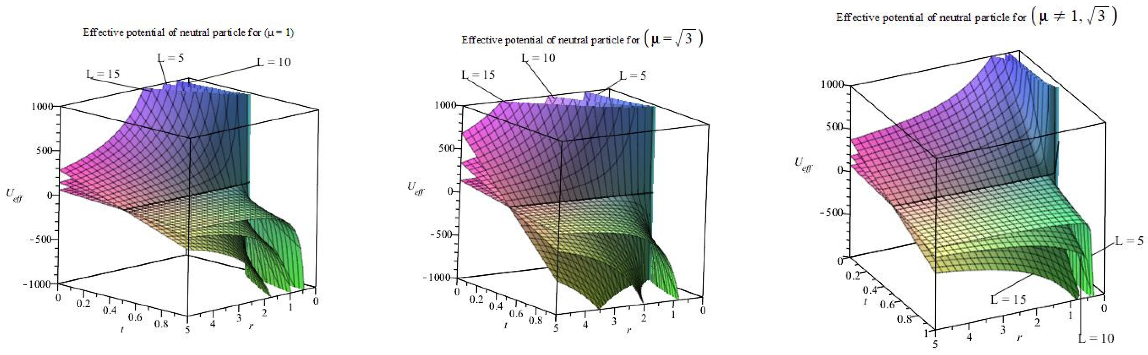
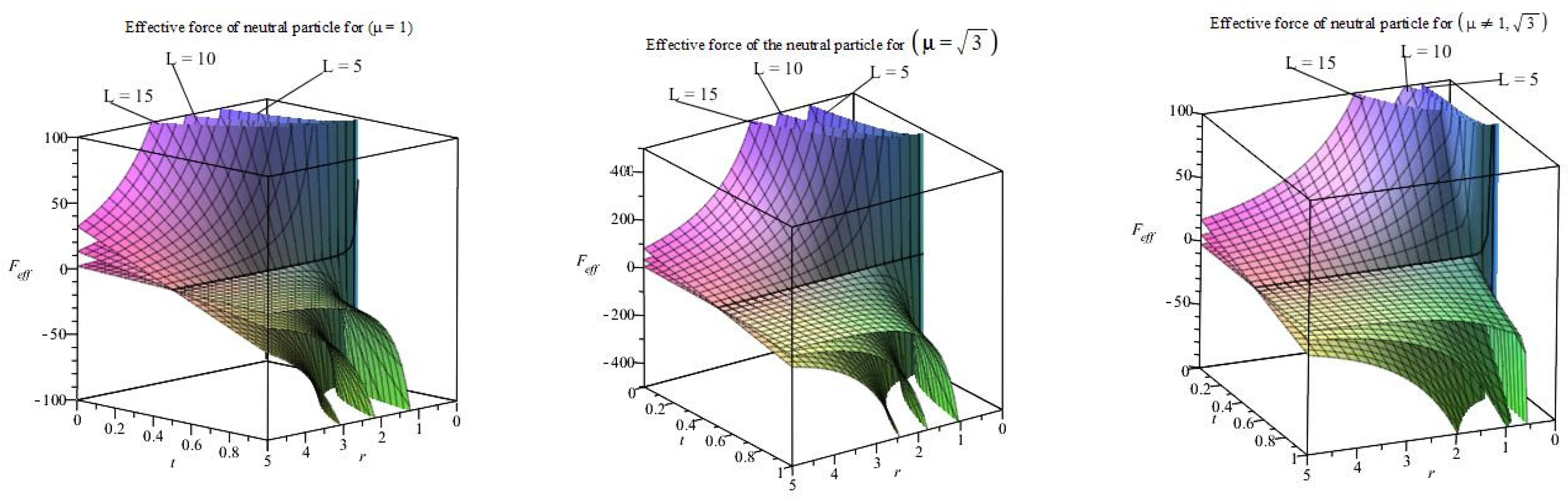
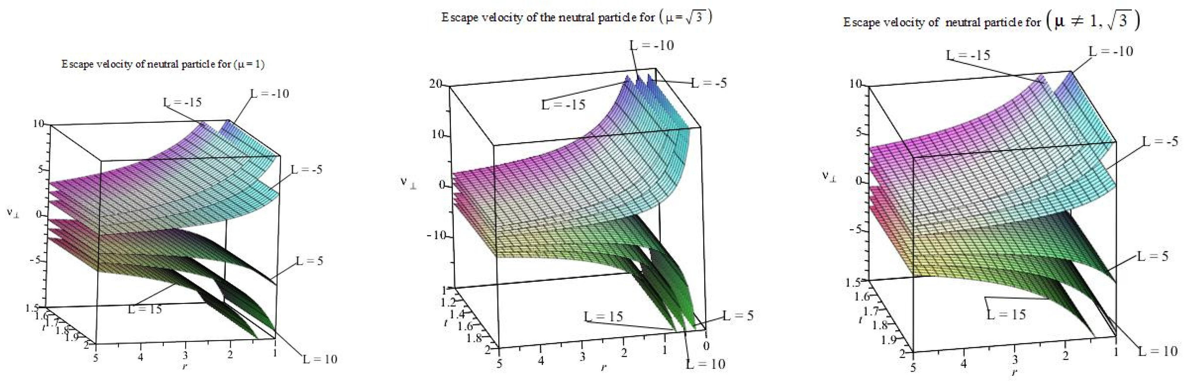
4. Dynamics of the Neutral Particle

Here, we find the escape velocity of the particle and analyze additional parameters such as $U_{eff}$, $L_z$, $F_{eff}$, and energy about particle’s motion around Dilaton BHs w.r.t time t. We also obtained the approximate energy $\left(E_{apprx}\right)$ and approximate angular momentum $\left(L_z\right)$ from Table 2 [38].

$$\begin{array}{ccc}\hfill E_{apprx}& =& (E-\frac{ϵs}{a})(1+\frac{ϵt}{a}),\hfill \\ \hfill L^2& =& \left(r^2{\nu }_{\perp }+\frac{L_z^2}{{sin}^2\theta }\right)\left(1+\frac{ϵt}{a}\right),\hfill \\ \hfill where{\nu }_{\perp }& =& {\dot{\theta }}^2{r}^2,E=X\left(r\right)\dot{t},{\dot{x}}_{\gamma }{\dot{x}}^{\gamma }=1.\hfill \end{array}$$

(52)

By using the normalized condition in Equation (52), we obtain

$$E^2-X\left(r\right)\left(\left(1-\frac{ϵt}{a}\right)+\frac{L_z^2\left(1-\frac{2ϵt}{a}\right)}{r^2{sin}^2\theta }\right)={\dot{r}}^2.$$

(53)

The effective potential for $\dot{r}=0$ and $\theta =\frac{\pi }{2}$ is given by

$$E^2=X\left(r\right)\left(1-\frac{ϵt}{a}+\frac{L_z^2\left(1-\frac{2ϵt}{a}\right)}{r^2}\right)=U_{eff}.$$

(54)

Assume that the particle collides with other particles and after the collision, we observed three possibilities: (i) escape to ∞, (ii) bounded around BHs, or (iii) captured by the BHs [35]. The results are based on the collision process. It is noticed that both energy and angular momentum are changed after collision [52]. We studied some constraints before the evaluation of this situation, and observe that the momentum and initial velocity are not changed, but energy is changed, which leads to the exploration of the particle dynamics. Thus, $U_{eff}$ becomes

$$U_{eff}=X\left(r\right)\left(\frac{{(L_z+r{\nu }_{\perp })}^2\left(1-\frac{2ϵt}{a}\right)}{r^2{sin}^2\theta }+\left(1-\frac{ϵt}{a}\right)\right)=E^2.$$

(55)

The energy of particles before a collision is less than that energy as colliding particles provide some energy to orbital particles after a collision. The escape velocity $\left({\nu }_{\perp }\right)$ can be found from Equation (55).

$${\nu }_{\perp }={\left(\frac{E^2\left(1+\frac{2ϵt}{a}\right)}{X\left(r\right)}-(1+\frac{ϵt}{a})\right)}^{\frac{1}{2}}-\frac{L_z}{r}.$$

(56)

Next, we examined the effective potential of neutral particles and describe energy conditions near the TC Dilaton BH. Figure 1 shows the behavior of $U_{eff}$ of neutral particles in the proximity of TC Dilaton BH for various values of $L_z$. The left panel of Figure 1 provides the minima of $U_{eff}$ for the values of $L_z$ = 5, 10, 15 at $r\approx 0.5,1,1.7$ for t $\in (0.5,1)$, while, the maxima of $U_{eff}$ for the values of $L_z$ = 5, 10, 15, at $r\approx 0.5,1,1.7$ for t $\in (0,0.5)$, which is a good agreement with [35]. New features for the dynamics of particles appear due to the Dilaton parameter. It is noticed that increasing the Dilaton parameter, $U_{eff}$ also increases and vice versa, which leads to the possibility that the particle may escape from the vicinity of BH. Hence, the Dilaton parameter plays a vital role in the motion of neutral particles.

Moreover, the effective force is given by

$$\begin{array}{ccc}\hfill F_{eff}& =& -\frac{1}{2}\frac{d{U}_{eff}}{dr}\hfill \\ \hfill & =& -\frac{1}{2}\left(X^{\prime }\left(r\right)\right)\left(1-\frac{ϵt}{a}+\frac{L_z^2\left(1-\frac{2ϵt}{a}\right)}{r^2}\right)+\frac{X\left(r\right)L_z^2\left(1-\frac{2ϵt}{a}\right)}{r^3}.\hfill \end{array}$$

We investigated the effective force of neutral particles around TC Dilaton BHs, in which attracting and repelling gravitational force generated by scalar vector tensor field which bound the particle’s motion towards the singularity as shown in Figure 2 [53]. A new feature appears due to Dilaton parameter, the effective force is increased considerably for higher values of Dilaton parameter and vice versa.

Finally, escape velocity is the most important property which provides the information about the fate of particle. The behavior of ${\nu }_{\perp }$ as a function of t and r is investigated for various values of $L_z$ in Figure 3. Escape velocity is increased, as we can see in middle panel for higher values as compare to lower values of Dilaton parameter. Hence, it can be summarized that the chances of particles escaping increase for higher values of Dilaton parameters, which provides a new signature as compared to angular momentum.

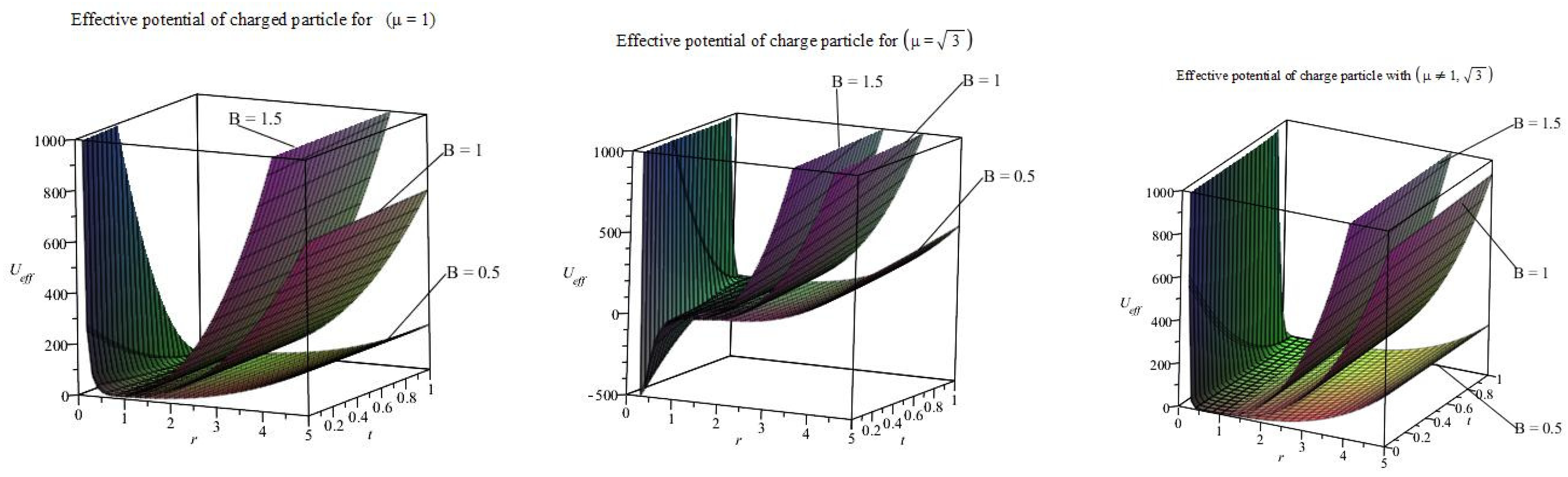
5. Dynamics of the Charged Particle

Assume that a particle motion and its electric charge q are affected by B in the BH exterior. Suppose that strength of B exists around the BH, which is axisymmetric and homogeneous at spatial infinity. For the construction of magnetic field B, we utilize the same techniques that are given in [34,35,36,37]. The $U_{eff}$ of test particles is given by

$$U_{eff}=X\left(r\right)\left({\left(\frac{L_z\left(1-\frac{ϵt}{a}\right)}{r^2{sin}^2\theta }-B\right)}^2{r}^2{sin}^2\theta +\left(1-\frac{ϵt}{a}\right)\right).$$

(57)

Using the equatorial plane conditions, we have

$$U_{eff}=X\left(r\right)\left(\left(1-\frac{ϵt}{a}\right)+r^2{\left(\frac{L_z\left(1-\frac{ϵt}{a}\right)}{r^2}-B\right)}^2\right).$$

(58)

Taking derivative of Equation (58) w. r. t r, we obtain

$$\begin{array}{ccc}\hfill \frac{d{U}_{eff}}{dr}& =& X^{\prime }\left(r\right)\left(1-\frac{ϵt}{a}+r^2{\left(\frac{(1-\frac{ϵt}{a})L_z}{r^2}-B\right)}^2\right)\hfill \\ \hfill & +& X\left(r\right)\left(2r{\left(\frac{L_z(1-\frac{ϵt}{a})}{r^2}-B\right)}^2-\frac{4\left(\frac{(L_z(1-\frac{ϵt}{a})}{r^2}-B\right)L_z(1-\frac{ϵt}{a})}{r}\right).\hfill \end{array}$$

(59)

After collision in the magnetic field $\left(\dot{r}=0and\theta =\frac{\pi }{2}\right)$, then $U_{eff}$ is

$$U_{eff}=E^2=X\left(r\right)\left(r^2{\left(\frac{({\nu }_{\perp }r+L_z)(1-\frac{ϵt}{a})}{r^2}-B\right)}^2+(1-\frac{ϵt}{a})\right).$$

(60)

The ${\nu }_{\perp }$ of particle is

$$\left(\sqrt{\frac{E^2}{X\left(r\right)}-(1-\frac{ϵt}{a})}+rB\right)(1+\frac{ϵt}{a})-\frac{L_z}{r}={\nu }_{\perp }.$$

(61)

Now, differentiating Equation (59) w.r.t r, we obtain

$$\begin{array}{ccc}\hfill \frac{d^2{U}_{eff}}{d{r}^2}& =& X^{″}\left(r\right)\left(1-\frac{ϵt}{a}+r^2{\left(\frac{L_z(1-\frac{ϵt}{a})}{r^2}-B\right)}^2\right)\hfill \\ \hfill & +& 2X^{\prime }\left(r\right)\left(2r{\left(\frac{L_z(1-\frac{ϵt}{a})}{r^2}-B\right)}^2-\frac{4\left(\frac{L_z(1-\frac{ϵt}{a})}{r^2}-B\right)L_z(1-\frac{ϵt}{a})}{r}\right)\hfill \\ \hfill & +& X\left(r\right)(2{\left(\frac{L_z(1-\frac{ϵt}{a})}{r^2}-B\right)}^2-\frac{4\left(\frac{L_z(1-\frac{ϵt}{a})}{r^2}-B\right)L_z(1-\frac{ϵt}{a})}{r^2}\hfill \\ \hfill & +& \frac{8L_z^2{(1-\frac{ϵt}{a})}^2}{r^4}).\hfill \end{array}$$

(62)

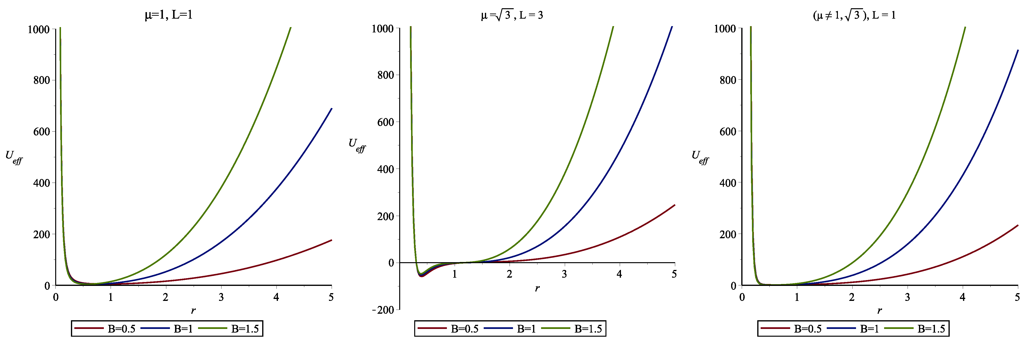
5.1. Behavior of the Effective Potential of the Charged Particle

The behavior of $U_{eff}$ as a function of r and t near the Dilaton BH was examined for various values of B. In all parts of the Figure 4 and Figure 5, we observed that $U_{eff}$ move toward the BH when time t increases. Thus, the chances of a particle moving toward a stable orbit increases in the presence of B. Here, we also observed that the presence of a small value of magnetic field at the minimum $U_{eff}$ is moving away from the horizon and decreased ISCO width as compared to the large values of B, which is similar to [33,54]. Hence, it is concluded that an increase in the magnetic field boosts the width of stable region. A new feature as for the dynamics of charged particle appears due to the Dilaton parameter. Further, it is noticed that the effective potential increases significantly for higher values of dilaton parameter $\left(\mu \right)$ and conversly. Therefore, the chances of escaping the particle is increased for higher values of the Dilaton parameter. Hence, It is worth mentioning that the Dilaton parameter plays a meaningful role in the particle dynamics of BH.

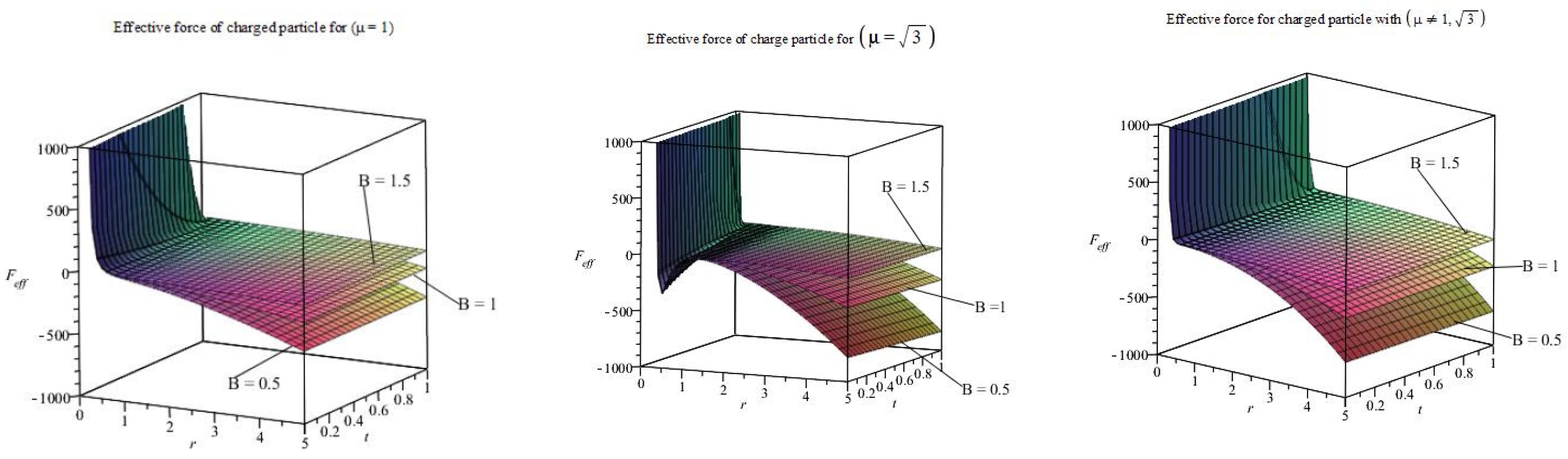
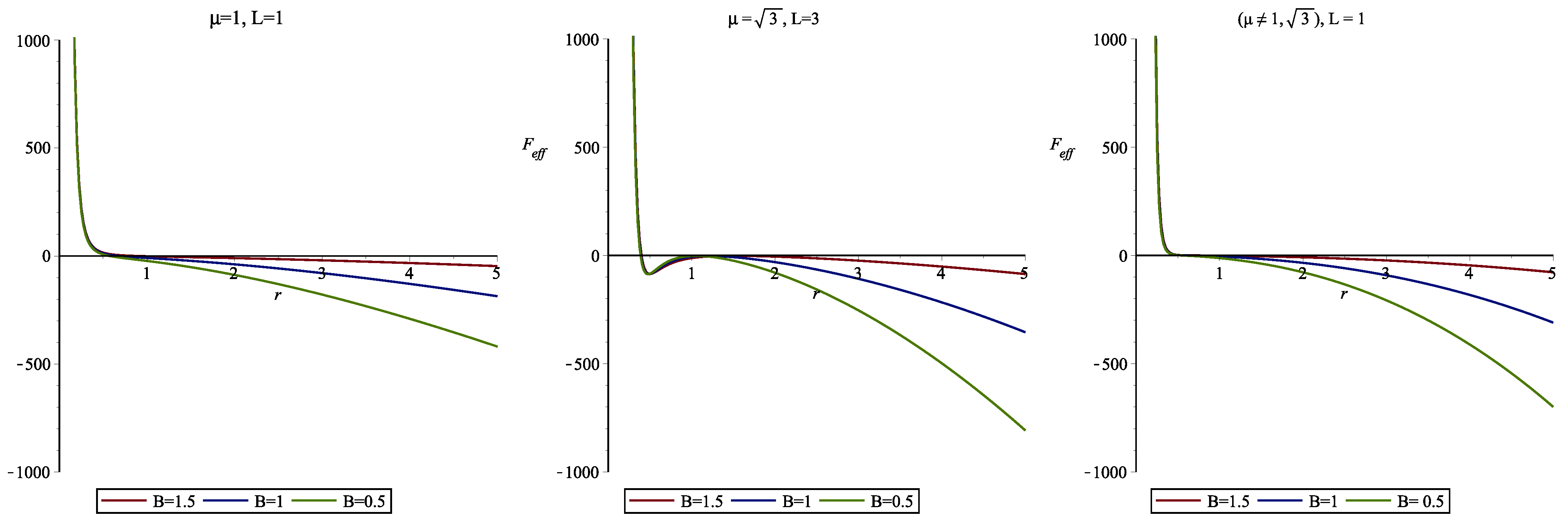
5.2. Behavior of the Effective Force of the Charged Particle

The $F_{eff}$ on the test particle is

$$\begin{array}{ccc}\hfill F_{eff}& =& -\frac{1}{2}\frac{d{U}_{eff}}{dr}\hfill \\ \hfill & =& -\frac{1}{2}\left(X^{\prime }\left(r\right)\right)\left(1-\frac{ϵt}{a}+r^2{\left(\frac{(1-\frac{ϵt}{a})L_z}{r^2}-B\right)}^2\right)\hfill \\ & -& \frac{1}{2}\left(X\left(r\right)\right)\left(2r{\left(\frac{L_z(1-\frac{ϵt}{a})}{r^2}-B\right)}^2-\frac{4\left(\frac{(L_z(1-\frac{ϵt}{a})}{r^2}-B\right)L_z(1-\frac{ϵt}{a})}{r}\right)\hfill \end{array}$$

(63)

Figure 6 and Figure 7 presents the behavior of $F_{eff}$ for different values of B as a function of t and r near the TC Dilaton BH. It is noticed that the $F_{eff}$ of the test particle is repulsive for small values of B as compared to large values. By increasing the Dilaton parameter, the effective force also increases. Hence, the chances to escape the particle are boosted for large values of the Dilaton parameter $\mu$ and magnetic field B.

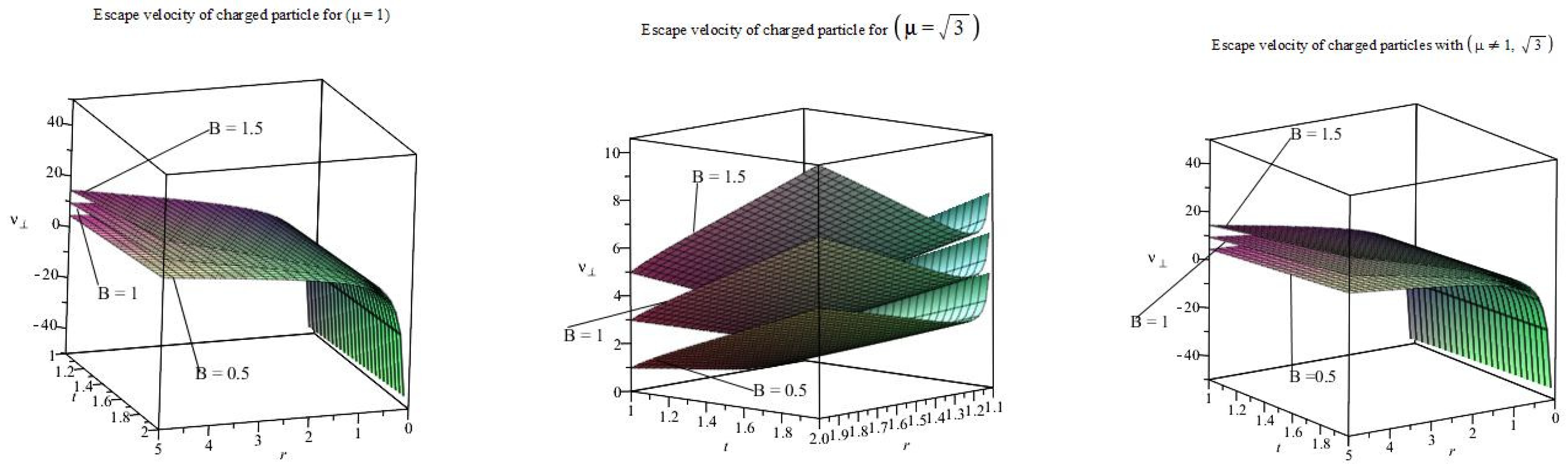
5.3. Behavior of the ${\nu }_{\perp }$ of the Charged Particle

The expression

$$\dot{\varphi }=-B+\frac{L_z(1-\frac{ϵt}{a})}{r^2{sin}^2\theta }.$$

(64)

implies that left side is -ve if the Lorentz force show attraction. The particle’s motion is in the clockwise direction and same from other side. Figure 8, Figure 9, Figure 10 and Figure 11 present the behavior of ${\nu }_{\perp }$ as function of t and r for various values of a magnetic field near the TC Dilaton BH. It is observed that the orbital motion of test particle is effected due to strong magnetic field; therefore, it is possible for the particle to escape from the grip of BH. The effect of the Dilaton parameter is more significant and gives fruitful results which are described as follows:

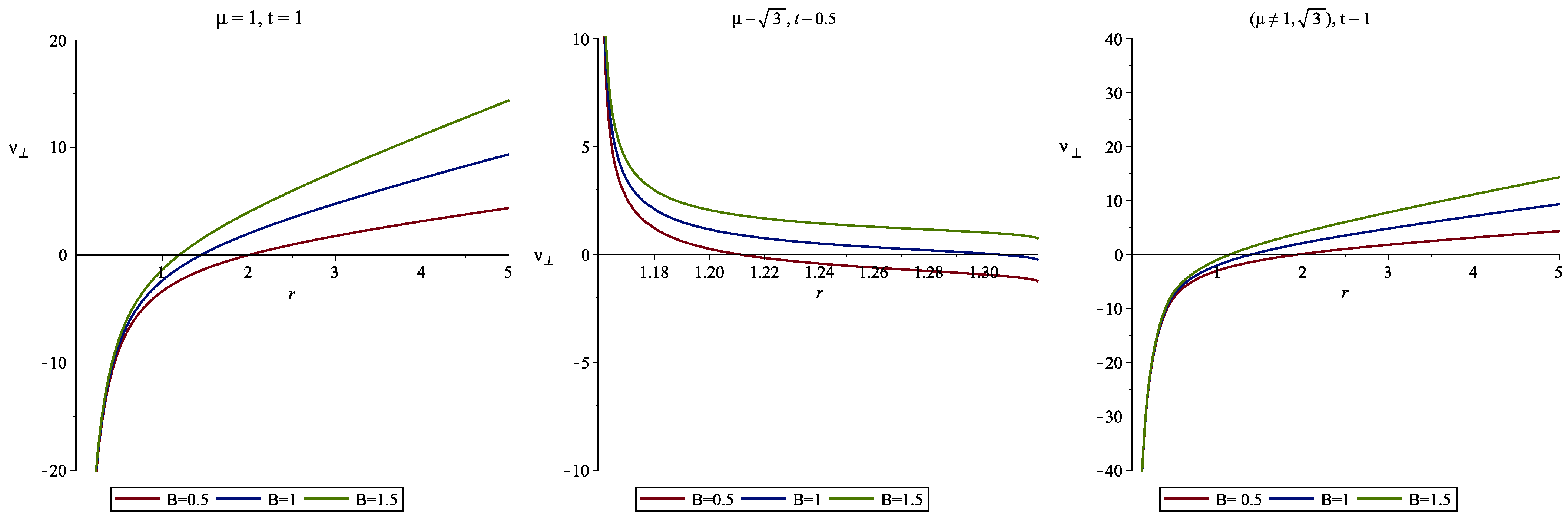
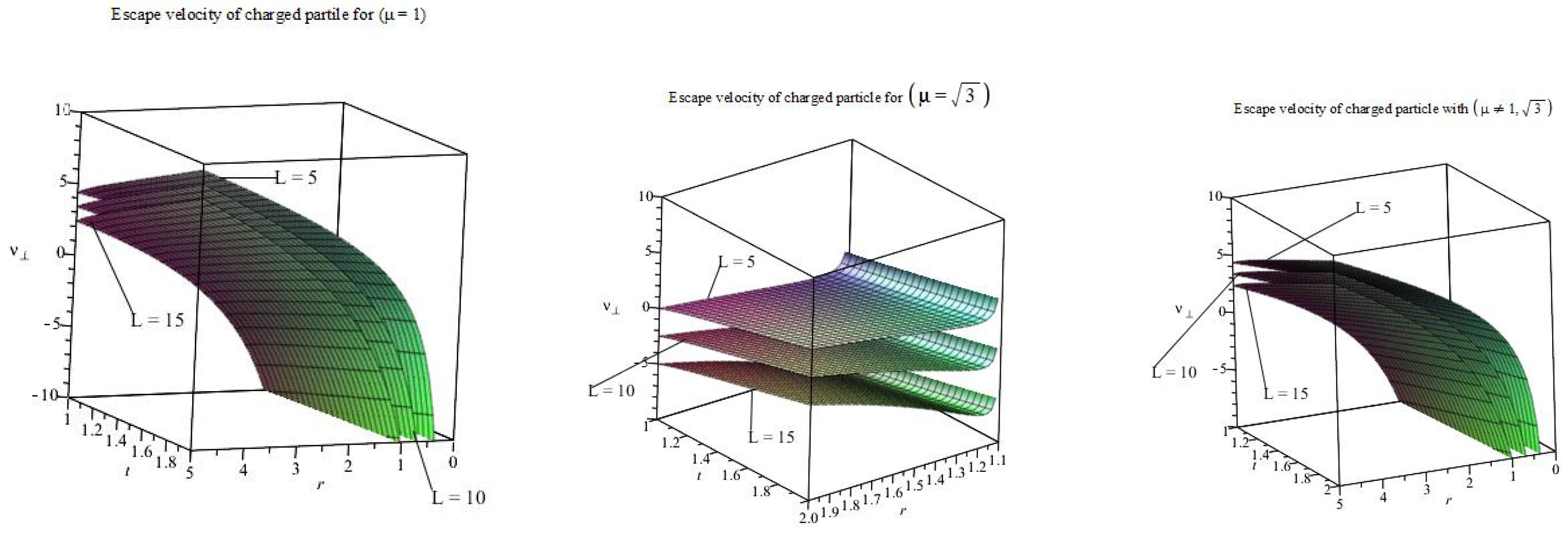
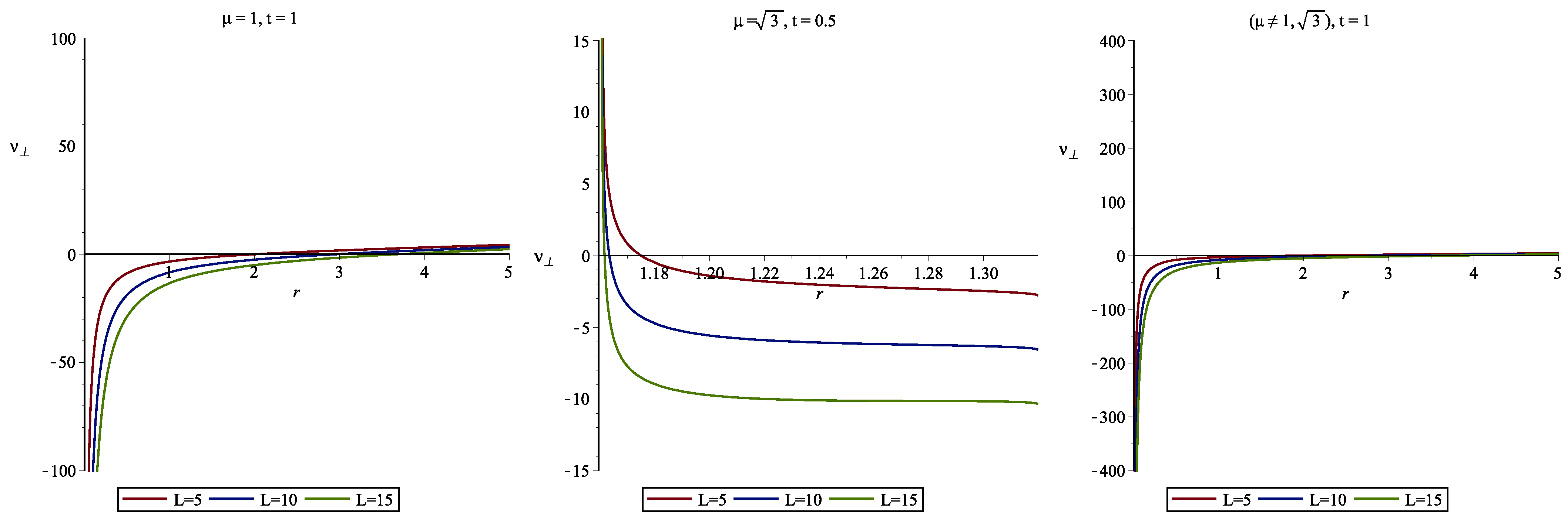
• For $\mu =0.64$, near the singularity, the escape velocity is very low, as radial distance and time increases, the escape velocity increases which is evidence.
• For $\mu =1$, the escape velocity is low for small radial distance, but it increases significantly as radial distance and time increases as compared to $\mu =0.64$.
• Interestingly, for $\mu =\sqrt{3}$, it is observed that the escape velocity is very high near the BH, which provides the evidence that the Dilaton parameter $\mu$ is modeled by the dark energy. Hence, the particle is repelled due to the effect of dark energy, so the chances of escape are very high near the BH.

6. Conclusions

In this work, we studied the motion of neutral and charged particles near TC Dilaton BHs in the presence and as well as absence of magnetic fields. The effect of the Dilaton parameter on the fate of particles moving around the TC Dilaton parameter was noted. Furthermore, the effect of B (magnetic field) and Dilaton parameter was examined on $U_{eff}$ (effective potential), $F_{eff}$ (effective force) and ${\nu }_{\perp }$ (escape velocity) of charged and neutral particles w.r.t. time. We concluded that the Dilaton parameter affects the motion of charge and chargeless particles; as the radial coordinate increases, those particles rigorously accelerate in the vicinity of compact objects. We also perceived the stern attraction and repulsion of neutral particles for various values of $L_z$ (angular momentum) and $\mu$ (Dilaton parameter) w.r.t. time. One can notice that ${\nu }_{\perp }$ is attractive for negative values of $L_z$ while it is repulsive for positive values of $L_z$. Interestingly, the nature of ${\nu }_{\perp }$ does not change w.r.t. time.

Additionally, in the motion of the charged particle, we detected that the minima of effective potential shifted towards the singularity, and the width of ISCO increases for a solid magnetic field compared to a weak magnetic field. A new feature for the dynamics of charged particles appears due to the Dilaton parameter. It is noted that the effective potential and effective force also enlarged significantly for higher values of Dilaton parameter $\left(\mu \right)$ and vice versa. Therefore, the chances of escaping the particle increase for higher values of the Dilaton parameter near the BH. Hence, it is worth mentioning that the Dilaton parameter plays a part and parcel role in the particle dynamics of BH. In an extended way, the Dilaton BH admits the time conformal factor by keeping the structure of symmetry [37], due to variation in time, the angular momentum and energy are lost by the BH in the outcome of this the geometry of BH change frequently, which explain the phenomena of gravitational waves.

References

- Green, M.B.; Schwarz, J.H.; Witten, E. Superstring Theory: Volume 2, Loop Amplitudes, Anomalies and Phenomenology; Cambridge University Press: Cambridge, UK, 2012. [Google Scholar]
- Gibbons, G.W.; Maeda, K.-I. Black holes and membranes in higher-dimensional theories with dilaton fields. Nucl. Phys. B 1988, 298, 741–775. [Google Scholar] [CrossRef]
- Dehghani, M.; Setare, M.R. Dilaton black holes with power law electrodynamics. Phys. Rev. D 2019, 100, 044022. [Google Scholar] [CrossRef]
- Dehghani, M. Thermodynamics of (2 + 1)-dimensional black holes in Einstein-Maxwell-dilaton gravity. Phys. Rev. D 2017, 96, 044014. [Google Scholar] [CrossRef]
- Dehghani, M. Nonlinearly charged scalar-tensor black holes in (2 + 1) dimensions. Phys. Rev. D 2019, 99, 104036. [Google Scholar] [CrossRef]
- Bekenstein, J.D. Nonexistence of baryon number for black holes. II. Phys. Rev. D 1972, 5, 2403. [Google Scholar] [CrossRef]
- Teitelboim, C. Nonmeasurability of the quantum numbers of a black hole. Phys. Rev. D 1972, 5, 2941. [Google Scholar] [CrossRef]
- Sheykhi, A.; Kazemi, A. Higher dimensional dilaton black holes in the presence of exponential nonlinear electrodynamics. Phys. Rev. D 2014, 90, 044028. [Google Scholar] [CrossRef]
- Dehghani, M. Thermal fluctuations of AdS black holes in three-dimensional rainbow gravity. Phys. Lett. B 2019, 793, 234–239. [Google Scholar] [CrossRef]
- Sheykhi, A.; Naeimipour, F.; Zebarjad, S.M. Phase transition and thermodynamic geometry of topological dilaton black holes in gravitating logarithmic nonlinear electrodynamics. Phys. Rev. D 2015, 91, 124057. [Google Scholar] [CrossRef]
- Dehghani, M. Thermodynamics of (2 + 1)-dimensional charged black holes with power-law Maxwell field. Phys. Rev. D 2016, 94, 104071. [Google Scholar] [CrossRef]
- Kashif, A.K.; Seadawy, A.R.; Jhangeer, A. Numerical appraisal under the influence of the time dependent Maxwell fluid flow over a stretching sheet. Math. Methods Appl. Sci. 2021, 44, 5265–5279. [Google Scholar]
- Lu, D.; Seadawy, A.; Arshad, M. Bright-Dark optical soliton and dispersive elliptic function solutions of unstable nonlinear Schrodinger equation and its applications. Opt. Quantum Electron. 2018, 50, 23. [Google Scholar] [CrossRef]
- Dehghani, M.; Hamidi, S.F. Thermal stability analysis of nonlinearly charged asymptotic AdS black hole solutions. Phys. Rev. D 2017, 96, 044025. [Google Scholar] [CrossRef]
- Hendi, S.H. Asymptotically charged BTZ black holes in gravity’s rainbow. Gen. Relativ. Gravit. 2016, 48, 50. [Google Scholar] [CrossRef]
- Hendi, S.H.; Panahiyan, S.; Panah, B.E.; Momennia, M. Thermodynamic instability of nonlinearly charged black holes in gravity’s rainbow. Eur. Phys. J. C 2016, 76, 150. [Google Scholar] [CrossRef]
- Dehghani, M. Thermodynamic properties of dilaton black holes with nonlinear electrodynamics. Phys. Rev. D 2018, 98, 044008. [Google Scholar] [CrossRef]
- Seadawy, A.R.; Asghar, A.; Wafaa, A.A. Analytical wave solutions of the (2 + 1)-dimensional first integro-differential Kadomtsev-Petviashivili hierarchy equation by using modified mathematical methods. Results Phys. 2019, 15, 102775. [Google Scholar] [CrossRef]
- Frolov, V.P.; Novikov, I.D. Black Hole Physics, Basic Concepts and New Developments; Springer: Berlin, Germany, 1998. [Google Scholar]
- Sharp, N.A. Geodesics in black hole space-times. Gen. Relativ. Gravit. 1979, 10, 659–670. [Google Scholar] [CrossRef]
- Chandrasekhar, S.; Subrahmanyan, C. The Mathematical Theory of Black Holes; Oxford University Press: Oxford, UK, 1998; Volume 69. [Google Scholar]
- Borm, V.C.; Spaans, M. The influence of magnetic fields, turbulence, and UV radiation on the formation of supermassive black holes. Astron. Astrophys. 2013, 553, L9. [Google Scholar] [CrossRef][Green Version]
- Maqsood, F.; Yousaf, Z.; Bhatti, M.Z. Electromagnetic field and spherically symmetric dissipative fluid models. Pramana 2022, 96, 105. [Google Scholar] [CrossRef]
- Yousaf, Z.; Bhatti, M.Z.; Naseer, T. Evolution of the charged dynamical radiating spherical structures. Ann. Phys. 2020, 420, 168267. [Google Scholar] [CrossRef]
- Bhatti, M.Z.; Yousaf, Z. Dynamical instability of charged self-gravitating stars in modified gravity. Chin. J. Phys. 2021, 73, 115–135. [Google Scholar] [CrossRef]
- Bhatti, M.Z.; Yousaf, Z. Dynamical variables and evolution of the universe. Int. J. Mod. Phys. 2017, 26, 1750029. [Google Scholar] [CrossRef]
- Znajek, R. On being close to a black hole without falling in. Nature 1976, 262, 270–271. [Google Scholar] [CrossRef]
- Seadawy, A.R.; Iqbal, M. Propagation of the nonlinear damped Korteweg-de Vries equation in an unmagnetized collisional dusty plasma via analytical mathematical methods. Math. Methods Appl. Sci. 2021, 44, 737–748. [Google Scholar] [CrossRef]
- Blandford, R.D.; Znajek, R.L. Electromagnetic extraction of energy from Kerr black holes. Mon. Not. R. Astron. Soc. 1977, 179, 433–456. [Google Scholar] [CrossRef]
- Koide, S.; Shibata, K.; Kudoh, T.; Meier, D.L. Extraction of black hole rotational energy by a magnetic field and the formation of relativistic jets. Science 2002, 295, 1688–1691. [Google Scholar] [CrossRef] [PubMed]
- Frolov, V.P.; Shoom, A.A. Motion of charged particles near a weakly magnetized Schwarzschild black hole. Phys. Rev. D 2010, 82, 084034. [Google Scholar] [CrossRef]
- Pugliese, D.; Quevedo, H.; Ruffini, R. Motion of charged test particles in Reissner-Nordström spacetime. Phys. Rev. D 2011, 83, 104052. [Google Scholar] [CrossRef]
- Al Zahrani, A.M.; Frolov, V.P.; Andrey, A.S. Critical escape velocity for a charged particle moving around a weakly magnetized Schwarzschild black hole. Phys. Rev. D 2013, 87, 084043. [Google Scholar] [CrossRef]
- Shahzad, M.U.; Jawad, A.; Ali, F.; Abbas, G. Dynamics of particle near time conformal slowly rotating Kerr black hole. Chin. J. Phys. 2022, 77, 620–631. [Google Scholar] [CrossRef]
- Jawad, A.; Ali, F.; Shahzad, M.U.; Abbas, G. Dynamics of particles around time conformal Schwarzschild black hole. Eur. Phys. J. C 2016, 76, 586. [Google Scholar] [CrossRef]
- Khan, A.S.; Ali, F. The dynamics of particles around time conformal AdS-Schwarzschild black hole. Phys. Dark Universe 2019, 26, 100389. [Google Scholar] [CrossRef]
- Khan, I.A.; Khan, A.S.; Islam, S.; Ali, F. Particles dynamics around time conformal quintessential Schwarzschild black hole. Int. J. Mod. Phys. D 2020, 29, 2050095. [Google Scholar] [CrossRef]
- Jawad, A.; Umair Shahzad, M. Particle dynamics around time conformal regular black holes via Noether symmetries. Int. J. Mod. Phys. D 2017, 26, 1750059. [Google Scholar] [CrossRef]
- Farhad, A. Conservation laws of cylindrically symmetric vacuum solution of Einstein field equations. Appl. Math. Sci. 2014, 8, 4697–4702. [Google Scholar]
- Farhad, A.; Tooba, F.; Sajid, A. Complete classification of spherically symmetric static space-times via Noether symmetries. Theor. Math. Phys. 2015, 184, 973–985. [Google Scholar]
- Farhad, A. New black hole solutions of Einstein field equations and their Riemann curvature tensors. Mod. Phys. Lett. A 2015, 30, 1550028. [Google Scholar]
- Capozziello, S.; Man’ko, V.I.; Marmo, G.; Stornaiolo, C. Tomographic Representation of Minisuperspace Quantum Cosmology and Noether Symmetries (arXiv: 0706.3018 [gr-qc]) S. Capozziello, A. Stabile and A. Troisi. Class. Quantum. Grav. 2007, 24, 2153. [Google Scholar] [CrossRef]
- Capozziello, S.; Noemi, F.; Daniele, V. New spherically symmetric solutions in f (R)-gravity by Noether symmetries. Gen. Relativ. Gravit. 2012, 44, 1881–1891. [Google Scholar] [CrossRef]
- Paliathanasis, A.; Basilakos, S.; Saridakis, E.N.; Capozziello, S.; Atazadeh, K.; Darabi, F.; Tsamparlis, M. New Schwarzschild-like solutions in f (T) gravity through Noether symmetries. Phys. Rev. D 2014, 89, 104042. [Google Scholar] [CrossRef]
- Tsamparlis, M.; Paliathanasis, A. Lie and Noether symmetries of geodesic equations and collineations. Gen. Relativ. Gravit. 2010, 42, 2957–2980. [Google Scholar] [CrossRef]
- Dehghani, M. Thermodynamics of new black hole solutions in the EinsteinMaxwell-dilaton gravity. Int. J. Mod. Phys. D 2018, 27, 1850073. [Google Scholar] [CrossRef]
- Dehghani, M.; Hamidi, S.F. Nonlinearly charged black holes in the scalar-tensor modified gravity theory. Phys. Rev. D 2017, 96, 104017. [Google Scholar] [CrossRef]
- Zangeneh, M.K.; Dehghani, M.H.; Sheykhi, A. Thermodynamics of topological black holes in Brans-Dicke gravity with a power-law Maxwell field. Phys. Rev. D 2015, 92, 104035. [Google Scholar] [CrossRef]
- Dehghani, M. Thermodynamics of novel charged dilaton black holes in gravity’s rainbow. Phys. Lett. B 2018, 785, 274–283. [Google Scholar] [CrossRef]
- Dehghani, M. Thermodynamics of charged dilatonic BTZ black holes in rainbow gravity. Phys. Lett. B 2018, 777, 351–360. [Google Scholar] [CrossRef]
- D’Inverno, R.A. Introducing Einstein’s Relativity. Introducing Einstein’s Relativity by RA D’Inverno; Oxford University Press: New York, NY, USA, 1992. [Google Scholar]
- Aliev, A.N.; Gal’tsov, D.V. Magnetized black holes. Sov. Phys. Uspekhi 1989, 32, 75. [Google Scholar] [CrossRef]
- Moffat, J.W. Scalar–tensor–vector gravity theory. J. Cosmol. Astropart. Phys. 2006, 2006, 4. [Google Scholar] [CrossRef]
- Hussain, S.; Hussain, I.; Jamil, M. Dynamics of a charged particle around a slowly rotating Kerr black hole immersed in magnetic field. Eur. Phys. J. C 2014, 74, 3210. [Google Scholar] [CrossRef]