
A Structural Characterisation of the Mitogen-Activated Protein Kinase Network in Cancer

 ,
, 
 and
and 
Abstract
:1. Introduction
2. Methods
2.1. Complex Network Analysis
| Algorithm 1 ER graph generation algorithm. | |
| Input: n, , p | |
| Output: | |
| ▹n nodes | |
| whiledo | |
| end while | |
| while not connected do | |
| ▹ the function is provided from NetworkX | |
| while do | |
| end while | |
| end while |
2.2. Mapping to Hallmarks of Cancer
3. Results
3.1. The MAPK Network in Cancer
3.2. Topological Organisation of the MAPK Network
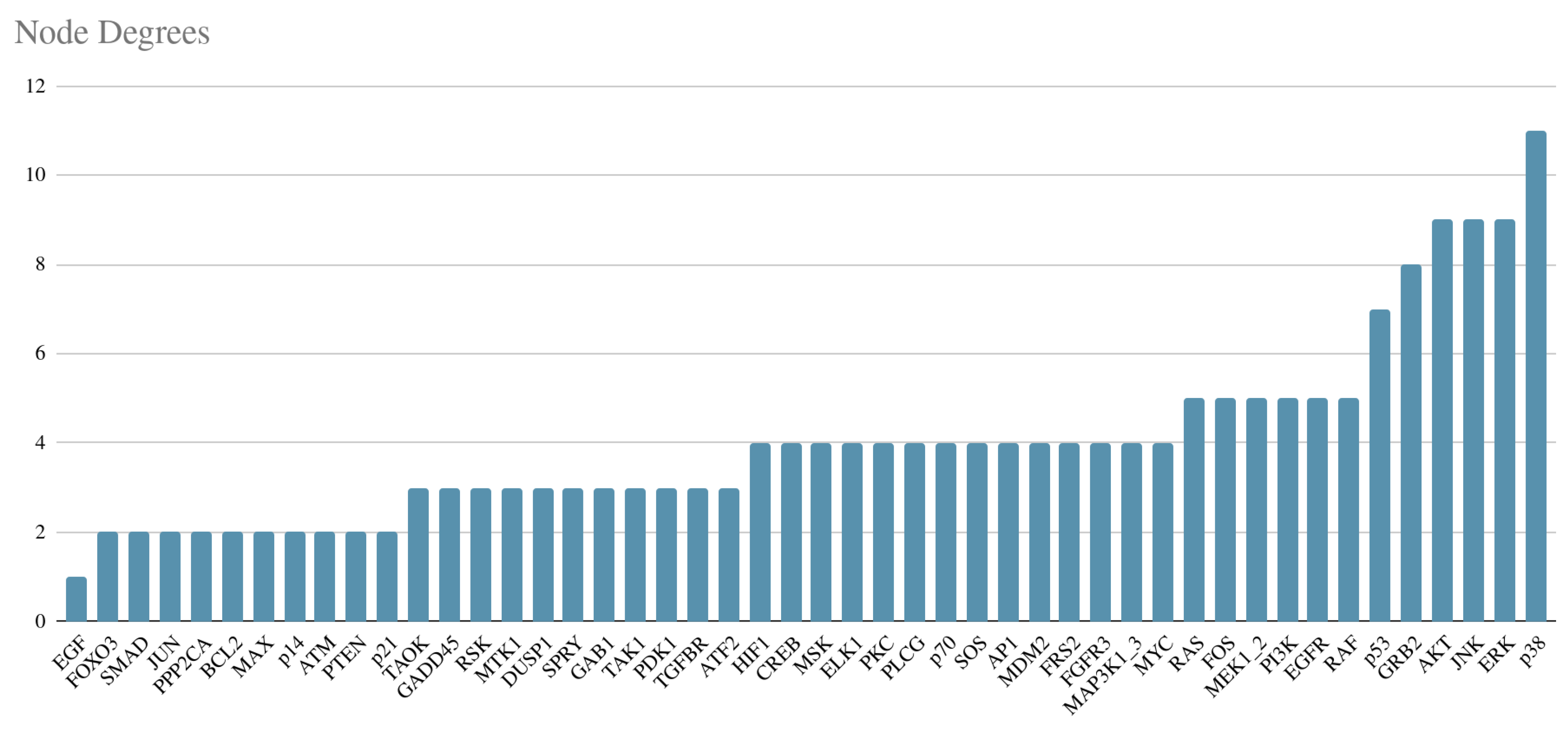
3.2.1. Degree Distribution
3.2.2. Community Detection
3.2.3. Complex Network Measures
3.3. Relationship with Hallmarks of Cancer
4. Discussion and Concluding Remarks
Supplementary Materials
Author Contributions
Funding
Institutional Review Board Statement
Informed Consent Statement
Acknowledgments
Conflicts of Interest
References
- Sung, H.; Ferlay, J.; Siegel, R.L.; Laversanne, M.; Soerjomataram, I.; Jemal, A.; Bray, F. Global cancer statistics 2020: GLOBOCAN estimates of incidence and mortality worldwide for 36 cancers in 185 countries. CA Cancer J. Clin. 2021, 71, 209–249. [Google Scholar] [CrossRef] [PubMed]
- Hanahan, D.; Weinberg, R.A. The hallmarks of cancer. Cell 2000, 100, 57–70. [Google Scholar] [CrossRef] [Green Version]
- Hanahan, D.; Weinberg, R.A. Hallmarks of cancer: The next generation. Cell 2011, 144, 646–674. [Google Scholar] [CrossRef] [PubMed] [Green Version]
- Frost, J.; Pienta, K.; Coffey, D. Symmetry and symmetry breaking in cancer: A foundational approach to the cancer problem. Oncotarget 2018, 9, 11429. [Google Scholar] [CrossRef] [Green Version]
- Bauer, R.; Kaiser, M.; Stoll, E. A computational model incorporating neural stem cell dynamics reproduces glioma incidence across the lifespan in the human population. PLoS ONE 2014, 9, e111219. [Google Scholar] [CrossRef] [Green Version]
- de Montigny, J.; Iosif, A.; Breitwieser, L.; Manca, M.; Bauer, R.; Vavourakis, V. An in silico hybrid continuum-/agent-based procedure to modelling cancer development: Interrogating the interplay amongst glioma invasion, vascularity and necrosis. Methods 2021, 185, 94–104. [Google Scholar] [CrossRef]
- Axenie, C.; Bauer, R.; Martínez, M.R. The Multiple Dimensions of Networks in Cancer: A Perspective. Symmetry 2021, 13, 1559. [Google Scholar] [CrossRef]
- Albert, R.; Othmer, H.G. The topology of the regulatory interactions predicts the expression pattern of the segment polarity genes in Drosophila melanogaster. J. Theor. Biol. 2003, 223, 1–18. [Google Scholar] [CrossRef]
- Karlsen, M.R.; Moschoyiannis, S. Evolution of control with learning classifier systems. Appl. Netw. Sci. 2018, 3, 30. [Google Scholar] [CrossRef]
- Papagiannis, G.; Moschoyiannis, S. Learning to Control Random Boolean Networks: A Deep Reinforcement Learning Approach. In Complex Networks 2019; Studies in Computational Intelligence; Springer: Cham, Swltzerland, 2019; Volume 881, pp. 721–734. [Google Scholar]
- Acernese, A.; Yerudkar, A.; Glielmo, L.; Del Vecchio, C. Reinforcement Learning Approach to Feedback Stabilization Problem of Probabilistic Boolean Control Networks. IEEE Control Syst. Lett. 2021, 5, 337–342. [Google Scholar] [CrossRef]
- Papagiannis, G.; Moschoyiannis, S. Deep Reinforcement Learning for Control of Probabilistic Boolean Networks. In Complex Networks 2020; Springer: Cham, Switzerland, 2020; Volume 944, pp. 361–371. [Google Scholar]
- Huang, S.; Ernberg, I.; Kauffman, S. Cancer attractors: A systems view of tumors from a gene network dynamics and developmental perspective. Semin. Cell Dev. Biol. 2009, 20, 869–876. [Google Scholar] [CrossRef] [PubMed] [Green Version]
- Jaeger, J.; Monk, N. Bioattractors: Dynamical systems theory and the evolution of regulatory processes. J. Physiol. 2014, 592, 2267–2281. [Google Scholar] [CrossRef] [PubMed]
- Dhillon, A.S.; Hagan, S.; Rath, O.; Kolch, W. MAP kinase signalling pathways in cancer. Oncogene 2007, 26, 3279–3290. [Google Scholar] [CrossRef] [PubMed] [Green Version]
- Grieco, L.; Calzone, L.; Bernard-Pierrot, I.; Radvanyi, F.; Kahn-Perles, B.; Thieffry, D. Integrative modelling of the influence of MAPK network on cancer cell fate decision. PLoS Comput. Biol. 2013, 9, e1003286. [Google Scholar] [CrossRef]
- Costa, L.d.; Rodrigues, F.A.; Travieso, G.; Boas, P.R.V. Characterization of complex networks: A survey of measurements. Adv. Phys. 2007, 56, 167–242. [Google Scholar] [CrossRef] [Green Version]
- Hagberg, A.; Swart, P.; Chult, D.S. Exploring Network Structure, Dynamics, and Function Using NetworkX; Technical Report; Los Alamos National Lab. (LANL): Los Alamos, NM, USA, 2008. [Google Scholar]
- Cherifi, H.; Palla, G.; Szymanski, B.; Lu, X. On community structure in complex networks: Challenges and opportunities. Appl. Netw. Sci. 2019, 4, 117. [Google Scholar] [CrossRef] [Green Version]
- Clauset, A.; Newman, M.E.; Moore, C. Finding community structure in very large networks. Phys. Rev. E 2004, 70, 066111. [Google Scholar] [CrossRef] [Green Version]
- Watts, D.; Strogatz, S. Collective dynamics of ‘small-world’ networks. Nature 1998, 393, 440–442. [Google Scholar] [CrossRef]
- Luce, R.D.; Perry, A.D. A method of matrix analysis of group structure. Psychometrika 1949, 14, 95–116. [Google Scholar] [CrossRef]
- Latora, V.; Marchiori, M. Efficient behavior of small-world networks. Phys. Rev. Lett. 2001, 87, 198701. [Google Scholar] [CrossRef] [Green Version]
- Erdos, P.; Rényi, A. On Random Graphs I. Publ. Math. 1959, 6, 290–297. [Google Scholar]
- Zhou, S.; Mondragón, R.J. The rich-club phenomenon in the Internet topology. IEEE Commun. Lett. 2004, 8, 180–182. [Google Scholar] [CrossRef] [Green Version]
- Csigi, M.; Kőrösi, A.; Bíró, J.; Heszberger, Z.; Malkov, Y.; Gulyás, A. Geometric explanation of the rich-club phenomenon in complex networks. Sci. Rep. 2017, 7, 1730. [Google Scholar] [CrossRef] [PubMed] [Green Version]
- Colizza, V.; Flammini, A.; Serrano, M.A.; Vespignani, A. Detecting rich-club ordering in complex networks. Nat. Phys. 2006, 2, 110–115. [Google Scholar] [CrossRef]
- Maslov, S.; Sneppen, K. Specificity and stability in topology of protein networks. Science 2002, 296, 910–913. [Google Scholar] [CrossRef] [Green Version]
- Maere, S.; Heymans, K.; Kuiper, M. BiNGO: A Cytoscape plugin to assess overrepresentation of Gene Ontology categories in Biological Networks. Bioinformatics 2005, 21, 3448–3449. [Google Scholar] [CrossRef] [Green Version]
- Nelson, M. mybinomtest. 2022. Available online: https://www.mathworks.com/matlabcentral/fileexchange/24813-mybinomtest-s-n-p-sided (accessed on 27 April 2022).
- Krishn, M.; Narang, H. The complexity of mitogen-activated protein kinases (MAPKs) made simple. Cell. Mol. Life Sci. 2008, 65, 3525–3544. [Google Scholar] [CrossRef]
- Voukantsis, D.; Kahn, K.; Hadley, M.; Wilson, R.; Buffa, F.M. Modeling genotypes in their microenvironment to predict single- and multi-cellular behavior. GigaScience 2019, 8, giz010. [Google Scholar] [CrossRef] [Green Version]
- Erdos, P.; Rényi, A. On the evolution of random graphs. Publ. Math. Inst. Hung. Acad. Sci 1960, 5, 17–60. [Google Scholar]
- Bauer, R.; Kaiser, M. Nonlinear growth: An origin of hub organization in complex networks. R. Soc. Open Sci. 2017, 4, 160691. [Google Scholar] [CrossRef] [Green Version]
- Wagner, E.F.; Nebreda, Á.R. Signal integration by JNK and p38 MAPK pathways in cancer development. Nat. Rev. Cancer 2009, 9, 537–549. [Google Scholar] [CrossRef] [PubMed]
- Bubici, C.; Papa, S. JNK signalling in cancer: In need of new, smarter therapeutic targets. Br. J. Pharmacol. 2014, 171, 24–37. [Google Scholar] [CrossRef] [PubMed]
- Maik-Rachline, G.; Hacohen-Lev-Ran, A.; Seger, R. Nuclear ERK: Mechanism of translocation, substrates, and role in cancer. Int. J. Mol. Sci. 2019, 20, 1194. [Google Scholar] [CrossRef] [PubMed] [Green Version]
- Martínez-Limón, A.; Joaquin, M.; Caballero, M.; Posas, F.; de Nadal, E. The p38 pathway: From biology to cancer therapy. Int. J. Mol. Sci. 2020, 21, 1913. [Google Scholar] [CrossRef] [Green Version]
- Liu, F.; Yang, X.; Geng, M.; Huang, M. Targeting ERK, an Achilles’ Heel of the MAPK pathway, in cancer therapy. Acta Pharm. Sin. B 2018, 8, 552–562. [Google Scholar] [CrossRef]
- Newman, M.E. The structure and function of complex networks. SIAM Rev. 2003, 45, 167–256. [Google Scholar] [CrossRef] [Green Version]
- de Anda-Jáuregui, G.; Alcalá-Corona, S.A.; Espinal-Enríquez, J. Functional and transcriptional connectivity of communities in breast cancer co-expression networks. Appl. Netw. Sci. 2019, 4, 22. [Google Scholar] [CrossRef] [Green Version]
- Kim, D.J.; Min, B.K. Rich-club in the brain’s macrostructure: Insights from graph theoretical analysis. Comput. Struct. Biotechnol. J. 2020, 18, 1761–1773. [Google Scholar] [CrossRef]
- Lazebnik, Y. What are the hallmarks of cancer? Nat. Rev. Cancer 2010, 10, 232–233. [Google Scholar] [CrossRef]
- Fouad, Y.A.; Aanei, C. Revisiting the hallmarks of cancer. Am. J. Cancer Res. 2017, 7, 1016. [Google Scholar]
- Buckley, A.M.; Lynam-Lennon, N.; O’Neill, H.; O’Sullivan, J. Targeting hallmarks of cancer to enhance radiosensitivity in gastrointestinal cancers. Nat. Rev. Gastroenterol. Hepatol. 2020, 17, 298–313. [Google Scholar] [CrossRef] [PubMed]
- Victori, P.; Buffa, F.M. The many faces of mathematical modelling in oncology. Br. J. Radiol. 2018, 92, 20180856. [Google Scholar] [CrossRef] [PubMed]
- Dessauges, C.; Mikelson, J.; Dobrzyński, M.; Jacques, M.A.; Frismantiene, A.; Gagliardi, P.A.; Khammash, M.; Pertz, O. Optogenetic actuator/ERK biosensor circuits identify MAPK network nodes that shape ERK dynamics. bioRxiv 2022. [Google Scholar] [CrossRef]
- Gibbs, D.L.; Shmulevich, I. Solving the influence maximization problem reveals regulatory organization of the yeast cell cycle. PLoS Comput. Biol. 2017, 13, e1005591. [Google Scholar] [CrossRef] [Green Version]
- Liu, Y.Y.; Slotine, J.J.; Barabási, A.L. Controllability of complex networks. Nature 2011, 473, 167. [Google Scholar] [CrossRef]
- Moschoyiannis, S.; Elia, N.; Penn, A.; Lloyd, D.J.B.; Knight, C. A web-based tool for identifying strategic intervention points in complex systems. Proc. Games for the Synthesis of Complex Systems (CASSTING @ ETAPS). EPTCS 2016, 220, 39–52. [Google Scholar] [CrossRef] [Green Version]


| Community | Genes |
|---|---|
| C1 | PPP2CA, MAP2K1, PI3K, RASA1, RAF, GAB1, FOS, RSK |
| MAP3K13, SOS1, ELK1, ERK | |
| C2 | GADD45, SMAD2, ATF2, AP1, JUN, TAK1, JNK, MTK1 |
| FOXO3, TGFBR1 | |
| C3 | P14, RPS6KB1, MAX, MYC, MDM2, PTEN, AKT, P21 |
| PDK1, P54 | |
| C4 | SPRYD1, FRS2, GRB2, PRKCA, PLCG1, FGFR3, EGFR |
| C5 | CREB, P38, MSK, DUSP1, TAOK1, BCL2, ATM |
| C6 | EGF, VEGF, HIF1 |
| Measure | Value | ER Network Value | Randomized Network Value |
|---|---|---|---|
| char path | 3.928 | 2.969 (std: 0.073) | 2.941 (std: 0.060) |
| modularity | 0.472 | 0.431 (std: 0.023) | 0.425 (std: 0.020) |
| clustering coefficient | 0.001 | 0.001 (std: 0.03) | 0.001 (std: 0.0002) |
| small-worldness | 0.993 | 0.986 (std: 0.298) | 1.173 (std: 0.305) |
| Degree | Normalized Value | Z-Score | p-Value |
|---|---|---|---|
| 2 | 0.981 | −1.325 | 0.092 |
| 3 | 0.956 | −0.936 | 0.175 |
| 4 | 0.602 | −2.342 | 0.009 |
| 5 | 0.189 | −2.754 | 0.003 |
| 6, 7, 8 | 0.0 | −2.401 | 0.008 |
| Hallmark | Shorthand |
|---|---|
| Self-sufficiency in growth signals | H1 |
| Insensitivity to anti-growth signals | H2 |
| Evading apoptosis | H3 |
| Limitless replicative potential | H4 |
| Sustained angiogenesis | H5 |
| Tissue invasion and metastasis | H6 |
| Reprogramming energy metabolism | H7 |
| Evading immune response | H8 |
| Community | Example GO Descriptions | Hallmarks (MOP) |
|---|---|---|
| C1 | reg. of apoptosis, | H3 (1.5), H6 (4.5⋆), H7 (1.13) |
| phosphorus metabolic process, | ||
| chemotaxis | ||
| C2 | regulation of apoptosis, | H3 (1.5), H7 (2.63⋆) |
| pos. reg. of metabolic process | ||
| C3 | response to extracellular stimulus, | H2 (6.0), H4 (6.0⋆) |
| reg. of cell cycle | ||
| reg. of cell cycle arrest | ||
| C4 | embryonic organ development, | H1 (4.8⋆), H7 (0.75) |
| tissue development, | ||
| phosphate metabolic process | ||
| C5 | reg. of apoptosis | H3 (3.0⋆), H7 (1.5⋆) |
| reg. of programmed cell death, | ||
| phosphate metabolic process | ||
| C6 | reg. of cell proliferation | H1(1.2), H5 (5.15⋆) |
| pos. reg. of angiogenesis | ||
| primitive heopoiesis |
Publisher’s Note: MDPI stays neutral with regard to jurisdictional claims in published maps and institutional affiliations. |
© 2022 by the authors. Licensee MDPI, Basel, Switzerland. This article is an open access article distributed under the terms and conditions of the Creative Commons Attribution (CC BY) license (https://creativecommons.org/licenses/by/4.0/).
Share and Cite
Chatzaroulas, E.; Sliogeris, V.; Victori, P.; Buffa, F.M.; Moschoyiannis, S.; Bauer, R. A Structural Characterisation of the Mitogen-Activated Protein Kinase Network in Cancer. Symmetry 2022, 14, 1009. https://doi.org/10.3390/sym14051009
Chatzaroulas E, Sliogeris V, Victori P, Buffa FM, Moschoyiannis S, Bauer R. A Structural Characterisation of the Mitogen-Activated Protein Kinase Network in Cancer. Symmetry. 2022; 14(5):1009. https://doi.org/10.3390/sym14051009
Chicago/Turabian StyleChatzaroulas, Evangelos, Vytenis Sliogeris, Pedro Victori, Francesca M. Buffa, Sotiris Moschoyiannis, and Roman Bauer. 2022. "A Structural Characterisation of the Mitogen-Activated Protein Kinase Network in Cancer" Symmetry 14, no. 5: 1009. https://doi.org/10.3390/sym14051009
APA StyleChatzaroulas, E., Sliogeris, V., Victori, P., Buffa, F. M., Moschoyiannis, S., & Bauer, R. (2022). A Structural Characterisation of the Mitogen-Activated Protein Kinase Network in Cancer. Symmetry, 14(5), 1009. https://doi.org/10.3390/sym14051009