Abstract
Skyline queries, which are based on the concept of Pareto dominance, filter the objects from a potentially large multi-dimensional collection of objects by keeping the best, most favoured objects in satisfying the user′s preferences. With today′s advancement of technology, ad hoc meetings or impromptu gatherings involving a group of people are becoming more and more common. Intuitively, deciding on an optimal meeting point is not a straightforward task especially when conflicting criteria are involved and the number of criteria to be considered is vast. Moreover, a point that is near to a user might not meet all the various users′ preferences, while a point that meets most of the users′ preferences might be located far away from these users. The task becomes more complicated when these users are on the move. In this paper, we present the Region-based Skyline for a Group of Mobile Users (RSGMU) method, which aims to resolve the problem of continuously finding the optimal meeting points, herein called skyline objects, for a group of users while they are on the move. RSGMU assumes a centroid-based movement where users are assumed to be moving towards a centroid that is identified based on the current locations of each user in the group. Meanwhile, to limit the searching space in identifying the objects of interest, a search region is constructed. However, the changes in the users′ locations caused the search region of the group to be reconstructed. Unlike the existing methods that require users to frequently report their latest locations, RSGMU utilises a dynamic motion formula, which abides to the laws of classical physics that are fundamentally symmetrical with respect to time, in order to predict the locations of the users at a specified time interval. As a result, the skyline objects are continuously updated, and the ideal meeting points can be decided upon ahead of time. Hence, the users′ locations as well as the spatial and non-spatial attributes of the objects are used as the skyline evaluation criteria. Meanwhile, to avoid re-computation of skylines at each time interval, the objects of interest within a Single Minimum Bounding Rectangle that is formed based on the current search region are organized in a Kd-tree data structure. Several experiments have been conducted and the results show that our proposed method outperforms the previous work with respect to CPU time.
1. Introduction
The skyline operator introduced by [1] plays an important role in accurately and efficiently solving problems that involve user preferences. Given a predefined set of evaluation criteria, the skyline operator is used to filter a set of interesting objects from a potentially large multi-dimensional collection of objects by keeping only those objects that are not worse than any other. The objects in the collection are assumed to be symmetric as they have symmetry properties (features) that are used to define the evaluation criteria. The dominant objects also known as skylines objects are said to be the best, most preferred set of objects. The process of computing skylines becomes challenging when conflicting criteria are involved and the number of criteria to be considered is vast. A classic example is searching for a hotel for a holiday that is cheap and near to a beach. Typically, hotels that are close to the beach are known to be expensive. While other criteria such as facilities, rating and service are equally important, distance and price are examples of conflicting criteria.
This paper presents the Region-based Skyline for a Group of Mobile Users (RSGMU) method, an extension of our previous work [2], which aims to continuously find the optimal meeting points for a group of users while they are on the move. In this work, these points are skyline objects derived from the objects that are within the search region of the group of users, also known as objects of interest. This is in line with today′s advancement of technology that shows ad hoc meetings or impromptu gatherings are becoming more and more common, yet deciding on a meeting or gathering point is not a straightforward task. RSGMU is capable of handling any collections of objects with symmetry properties, such as restaurants, hotels, cafes, shopping malls and parks, which can be used as a meeting or gathering place. The difference between RSGMU and SGMU [2] lies on the way the spatial and non-spatial preferences of the users is treated. In SGMU, these preferences are handled separately, which results in disjoint sets of skyline objects. The dominated objects based on spatial preferences are derived from the objects of interest, while the whole collection of objects in the space is analysed to identify the dominated objects based on non-spatial preferences. Although SGMU will not miss any important objects with regard to the non-spatial preferences of the users, the objects that are not within the search region will obviously not fulfilling the spatial preferences of these users.
There are several existing skyline derivation solutions; however, most of them are limited due to the following: (i) Although users are assumed to be on the move, their solutions are tailored made for fulfilling the preferences of a single user [3]; and (ii) approaches that are designed for computing skylines for a group of users make use of the initial location of the users in the skyline computation [4,5,6]. This means the skyline objects are not updated as users are assumed to be static. Nonetheless, considering the movement of users requires a mechanism to continuously update the skylines as these skylines might no longer be relevant to the users. In addition, the following common challenges were aimed to be resolved by earlier solutions [3,4,5,6]: (i) The task of identifying skyline objects for a group of users is not straightforward as many criteria need to be considered; and (ii) an object of interest that is near to the users might not meet all the various users′ preferences, while an object with facilities that meet most of the users′ preferences might be located far away from these users. The unique challenge aimed by RSGMU is to derive skylines that satisfy both the spatial and non-spatial preferences of a group of users while they are on the move. An object that was initially in the top list of the group of users might no longer be the object of interest once the users have moved away from their initial locations. Hence, a method is critically needed to not only continuously derive and update the skyline objects based on the changes in the users′ locations, but to also derive these objects that would assist the users to foresee the potential meeting points ahead of time.
The following scenario illustrates the problem tackled in this paper. It is assumed that there are 15 distinct objects representing objects of interests. Additionally, it is assumed that the search region is based on the initial locations of a group of users, , at time , as shown in Figure 1a, while the search region based on the changes in the users′ locations, , after a specified time interval, say , as is shown in Figure 1b. For simplicity, these users are not depicted in the figure. Ideally, the objects that fall within , i.e., , , , , , , , and , are compared to filter the dominant objects in fulfilling the preferences of the group of users. Let us say that the dominated objects within at time are , , , and . If none of these objects are chosen as a meeting point at time , then the changes in the users′ locations will result in changes in the search region, as shown in Figure 1b. Intuitively, the set of objects that falls within , i.e., , , , , is a subset of the set of objects of , and there are objects that are within but not within . Consequently, the pairwise comparisons performed earlier between the objects , , , and are pointless. Hence, in deriving the skylines for a group of users while they are on the move, it is crucial to predict the locations of these users in a specified time interval to avoid unnecessary pairwise comparisons.
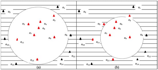
Figure 1.
Example of (a) a search region based on the initial locations and (b) search region based on the new locations of a group of users.
In general, the main contributions of this work can be briefly described as follows:
- We formally introduce the problem of finding the optimal meeting points, also known as skylines, of a group of users who are on the move and justify the significance of addressing the problem. In general, the optimal meeting points, i.e., skyline objects, that best meet the spatial and non-spatial preferences of the users are identified at a specified time interval until, finally, a skyline object is selected by the group of users as a meeting point. Several definitions are formally put forward, which include properties of a user, properties of an object, dominance, non-spatial dominance, spatial dominance, dominance in a space, skylines of a space, region of interest, search region, and object of interest.
- We propose an efficient solution, named Region-based Skyline for a Group of Mobile Users (RSGMU) method, which is designed mainly for deriving skyline objects for a group of users while they are on the move. RSGMU assumes a centroid-based movement where users are assumed to be moving towards a centroid. Unlike previous works [3,4,7,8,9,10] that require users to frequently report their latest locations, RSGMU utilises the dynamic motion formula to predict the locations of the users at a specified time interval, which results in the skyline objects being continuously updated. In addition, the skyline results are derived in advance before the users have actually arrived at the location. Meanwhile, to avoid re-computation of skylines at each time interval, the objects of interest are organized in a Kd-tree data structure.
- We conduct extensive experiments with various parameter settings to prove RSGMU′s capabilities in deriving the skyline objects for a group of users while they are on the move. These parameter settings are time interval, number of objects, data dimensionality, density, space size, number of users in a group, number of groups of users, and number of skyline objects.
This paper is organised as follows: Section 2 reviews the methods proposed by previous studies that are related to the work presented in this paper. Section 3 introduces the notations and deliberates the terms that are frequently used throughout the paper. It also presents the problem tackled by this paper. This is followed by Section 4, which presents the proposed method, RSGMU. This section focuses on the steps to be performed in order to achieve the main aim of the work. Section 5 evaluates the performance of the proposed method and compares the results to other previous work. The last section, Section 6, concludes this work and sheds light on some directions that can be pursued in the future.
2. Related Works
A great number of skyline algorithms have been proposed since the introduction of skyline operator by [1]. Among the most notable skyline algorithms are Block Nested-Loop (BNL) [1], Divide-and-Conquer (D&C) [1], Bitmap [11], Index [11], Nearest Neighbor (NN) [12], Branch and Bound Skyline (BBS) [13], Sort-Filter-Skyline (SFS) [14], Linear Elimination Sort for Skyline (LESS) [15], and Sort and Limit Skyline algorithm (SaLSa) [16]. This list is non exhaustive as more advanced skyline algorithms can be found in the literature [17], each concerned with various distinct issues. These include Bucket [18], Iskyline [18], Incoskyline [19], and OIS [20,21], which were developed to tackle issues related to incompleteness of data. Meanwhile, DyIn-Skyline [22] is an example of an algorithm that is meant for handling both the issues of incompleteness and changes in data; Skyline [23] is an extension of DyIn-Skyline and focuses on the changing state and structure of a database. On the other hand, BBIS [24], SkyQUD [25], and SQUiD [26] are algorithms meant for imprecise data, also known as uncertain data.
Of pertinence to the problem highlighted in this paper, we categorised the existing skyline algorithms into three categories, namely: (i) skyline queries for a mobile user, (ii) skyline queries for a group of static users, and (iii) skyline queries for a group of mobile users. Similar to our solution, the works reported here are those that assumed non-moving objects except for some studies such as [3,9], in which both static and moving objects are covered.
2.1. Skyline Queries for a Mobile User
A continuous skyline query processing strategy is proposed by [8] using the kinetic data structure for moving query points. The spatiotemporal coherence is analysed in order to avoid the need to compute the skyline from scratch at every time instance. The skyline query result is updated and available continuously. Meanwhile, to resolve the problem related to range-based skyline queries (RSQ), [9] proposed two algorithms named I-SKY, an index-based RSQ algorithm, and N-SKY, a non-index RSQ algorithm. Meanwhile, to resolve the problem related to continuous RSQ query, the incremental construction of the I-SKY index was devised. They also studied the probabilistic RSQ query problem. Their work is comprehensive such that both static and moving objects were covered. In addition, the work by [10] focused on the authentication problem of continuous location-based arbitrary-subspace skyline queries (LASQs). They developed a prefetching-based approach that enables clients to compute new LASQ results locally during movement, without frequently contacting the server for query re-evaluation. On the other hand, [3] studied the problem of range-based skyline queries (CRSQs) in road networks, where two algorithms named landmark-based (LBA) and index-based (IBA) were proposed. Furthermore, to handle continuous range-based skyline queries over moving objects, incremental versions of LBA and IBA were introduced. Nonetheless, [7] argued that the existing approaches for the continuous skyline query limit the area of the skyline query to a specific area in the road network; hence, not many useful query results can be retrieved. To reduce the number of intersection nodes in the road network, three algorithms were proposed, namely, intersection node aggregation algorithm (INAA), link remolding algorithm (LMA), and link fitting algorithm (LFA).
2.2. Skyline Queries for a Group of Static Users
The Spatial Skyline Queries (SSQ) was introduced by [4]. SSQ retrieves the objects that are not dominated by other objects based on spatial domination, i.e., the point′s distance to a query point. Three algorithms were proposed, namely, R-tree-based Branch-and-Bound Spatial Skyline (B2S2) and Voronoi-based Spatial Skyline (VS2) for static query points and Voronoi-based Continuous SSQ (VCS2) for streaming query points. This work was then extended in [5] for spatial network databases. Two algorithms were proposed, namely, SNS2 and VSNS2, which compute the spatial skyline with respect to the network distance in a spatial network database. Later, [6] proposed a new index structure, termed VoR-Tree, which incorporates Voronoi diagram and Delaunay graph of a set of objects into an R-tree that indexes their geometries. The data structure is experimented on various Nearest Neighbour (NN) queries that include kNN, Reverse kNN, k Aggregate NN, and spatial skyline queries on point data.
Meanwhile, ref. [27] considered spatial skyline query for a group of users having different positions. The final skyline results were obtained by utilising the non-spatial features and spatial features of the objects. The proposed method selects a set of spatial objects whose location for the group is not dominated by another spatial objects, which is then computed using the VoR-Tree. Having a similar aim as [27], an algorithm named VR (Voronoi and R-tree) was proposed by [28] for computing skyline of spatial objects for a group of users located at different locations. Both spatial features and non-spatial features of the objects were considered, while the VoR-tree and Sum Distance were utilised to calculate the spatial skyline objects. In 2018, ref. [29] proposed a solution for spatial skyline query over imperfect data for a set of query points located in different locations.
With a slightly different aim, refs. [2,30] proposed the RSGU method that avoids rescanning the set of objects within an area that has been explored during the skyline computation of previous groups of users. By partitioning each region into smaller units called fragments, the overlapping areas are determined, while the results of computing the skylines of each fragment, known as fragment skylines, are saved and utilised in the subsequent requests.
2.3. Skyline Queries for a Group of Mobile Users
The only work that falls under this category is the work conducted by [4]. In [4], the Voronoi-based Continuous SSQ (VCS2) was proposed for streaming query points, , whose points change location over time (i.e. mobile). The spatial skyline was updated by exploiting the pattern of change in to avoid unnecessary recomputation of the skyline.
Table 1 summarises the works reported in Section 2.1, Section 2.2, Section 2.3. From the table, the following can be observed:
- (a)
- Works that focus on continuous skyline query for a single user [3,7,8,9,10] assumed an arbitrary movement. In these methods, the user is required to frequently update their latest location.
- (b)
- The works by [2,5,6,27,28,29,30] that focus on non-continuous skyline query for a group of users used the initial locations of the users in determining the skyline objects. Hence, the type of movement either arbitrary or centroid-based was not significant in those studies. However, users in the group can always update their locations by submitting a new query.
- (c)
- Continuous skyline query for a group of users as studied by [4] assumed an arbitrary movement where users are required to frequently update their latest locations.
- (d)
- Most of the works used the spatial attributes of the users as well as the spatial and non-spatial attributes of the objects in obtaining the skyline objects [2,3,7,8,9,10,27,28,29,30], except for the works by [4,5,6], in which the non-spatial attributes of the objects were not taken into consideration. Hence, [4,5,6] defined skyline objects as those objects that best meet the spatial preferences of the group of users.
- (e)
- Our proposed method, RSGMU, differs from the works reported in this paper regarding the following: (i) RSGMU assumes a centroid-based movement to ensure that the travelling distance of each user is almost the same, so that they are able to meet on time. (ii) Unlike [2,4,6,27,28,29,30], which utilised a specific data structure to organise the objects in the whole space, RSGMU uses Kd-tree to organise the identified objects of interest that fall within a certain subspace. Hence, the changes in the users′ locations involve a smaller number of objects to be traversed. (iii) RSGMU utilises the dynamic motion formula to predict the locations of the users at a specified time interval, which results in the skyline objects to be continuously updated. On the other hand, users are required to frequently update their latest locations in [3,4,7,8,9,10] in order to continuously update the skyline objects. (iv) Although most works [2,3,7,8,9,10,27,28,29,30] used the spatial attributes of the users as well as the spatial and non-spatial attributes of the objects in obtaining the skyline objects, they are limited as their solutions are unable to cater the movement of the users.

Table 1.
Summary of the related works.
Table 1.
Summary of the related works.
| Author | Skyline Algorithm | Evaluation Criteria | Type of Query | Method of Tracking User′s Location | Data Structure Used | Single/ Group | Type of Movement | ||
|---|---|---|---|---|---|---|---|---|---|
| User | Object | ||||||||
| Spatial | Spatial | Non- Spatial | |||||||
| [8] | Continuous Skyline Query | √ | √ | √ | Continuous skyline query | Update | Kinetic | Single | Arbitrary |
| [9] | I-SKY, N-SKY, Incremental I-SKY | √ | √ | √ | Range-based skyline query (RSQ), continuous RSQ, Probabilistic RSQ query | Update | × | Single | Arbitrary |
| [10] | Location-based arbitrary-subspace skyline queries (LASQs) | √ | √ | √ | Continuous range-based skyline query | Update | × | Single | Arbitrary |
| [3] | Landmark-based (LBA), index-based (IBA) | √ | √ | √ | Continuous range-based skyline query | Update | × | Single | Arbitrary |
| [7] | Intersection node aggregation algorithm (INAA), link remolding algorithm (LMA), link fitting algorithm (LFA) | √ | √ | √ | Continuous range-based skyline | Update | × | Single | Arbitrary |
| [4] | Branch-and-Bound Spatial Skyline (B2S2), Voronoi-based Spatial Skyline (VS2), Voronoi-based Continuous SSQ (VCS2) | √ | √ | × | Spatial skyline query (SSQ), Continuous SSQ | Update | R-tree, Voronoi diagram | Group | Arbitrary |
| [5] | SNS2, VSNS2 | √ | √ | × | Spatial skyline query | × | × | Group | × |
| [6] | Voronoi-based and R-tree Spatial Skyline (VoR-Tree) | √ | √ | × | Spatial skyline query | × | Voronoi diagram, Delaunay graph | Group | × |
| [27] | VR (Voronoi and R-tree) | √ | √ | √ | Spatial skyline query | × | R-tree, Voronoi diagram | Group | × |
| [28] | VR (Voronoi and R-tree) | √ | √ | √ | Spatial skyline query | × | R-tree and Voronoi diagram | Group | × |
| [29] | Group Skyline Algorithm (GSA) | √ | √ | √ | Imperfect spatial skyline query | × | R-tree and Voronoi diagram | Group | × |
| [2,30] | Region-based Skyline for a Group of Users (RSGU) | √ | √ | √ | Spatial skyline query | × | R-tree, fragment | Group | × |
| Our Method | Region-based Skyline for a Group of Mobile Users (RSGMU) | √ | √ | √ | Continuous SSQ | Predict/ Update | Kd-tree | Group | Centroid-based |
3. Preliminaries
In this section, the important concepts and terms that are related to the work presented in this paper are explained, while the notations used throughout the paper are introduced. This is then followed by the descriptions of the problem tackled in this paper.
3.1. Definitions and Notations
Considering a data set , where is a list of users, is a list of objects, and where representing a spatial attribute, while is a set of non-spatial attributes.
The following definitions define the properties of a user and an object as used in this work.
Definition 1.
Properties of a User: Each user, , is associated with a spatial attribute that represents the location of the user at a certain time, . This is denoted as . For instance, ofTable 2denotes the location of user . Throughout this paper, the notations , and are associated with the initial state, current state and final state, respectively, of a user. The final state indicates that a skyline object has been selected. In this work, the initial location of a user, , i.e., at time , is assumed given while their subsequent locations are predicted using the dynamic motion formula in [31]. We used the notations to represent the sequence of iterations followed in predicting the locations of the users where and each , , is associated with a specific time. Hence, the terms iteration and time are used interchangeably in this paper. Here, the amount of time between two adjacent iterations is provided by a specified time interval, . For instance, if s, then the difference between the iterations and is s. It is also assumed that each user, , is moving with a constant speed of .
Definition 2.
Properties of an Object: Each object has two main elements denoted by whereis the value of spatial attribute (location), , and is a set of values of non-spatial attributes, , associated with. The location of an object is denoted as . As each object is assumed to be static, thus the location of the object is fixed regardless the changes in time. Hence, can be written as . For instance, the object ofTable 3can be written as .
Table 2.
The spatial attribute of a group of users, , at time .
Table 2.
The spatial attribute of a group of users, , at time .
| ID | Location |
|---|---|
| u1 | (2, 6) |
| u2 | (1.6, 3.2) |
| u3 | (6, 3.2) |
Table 3.
The spatial and non-spatial attributes of the objects.
Table 3.
The spatial and non-spatial attributes of the objects.
| ID | Location | Rating | Fee | ID | Location | Rating | Fee |
|---|---|---|---|---|---|---|---|
| (8, 6) | 2 | 80 | (14, 9) | 2 | 90 | ||
| (1, 4) | 2 | 80 | (8, 1) | 3 | 95 | ||
| (1, 2) | 3 | 80 | (5.9, 5.8) | 2 | 100 | ||
| (8, 8) | 1 | 60 | (4, 8) | 3 | 95 | ||
| (7, 3) | 2 | 90 | (2, 7) | 3 | 92 | ||
| (6, 6) | 2 | 80 | (−2, 9) | 3 | 100 | ||
| (3.1, 4) | 3 | 65 | (5, 7) | 2 | 93 | ||
| (10, 3.5) | 3 | 65 |
The following definitions define the notion of dominance in this work.
Definition 3
Dominance: Given two objects and where , is said to dominate (denoted by if and only if both of the following conditions hold: (1) non-spatially dominates and (2) spatially dominates . Without loss of generality, the definition is applicable for a given bounded space, , i.e., is a set of objects in the space . Similar note applies for Definition 4 and Definition 5.
Definition 4.
Non-spatial dominance: Given two objects and where , is said to non-spatially dominate (denoted by if and only if is no worse than (in this definition, greater value is preferable) in all the non-spatial attributes, . This is formally written as follows: if and only if . For instance, given = ((6, 6), {2, 80}) and = ((10, 3.5), {3, 65}), since is better than in both the dimensions Rating and Price, with the assumption that a higher rating and lower fee are preferable.
Definition 5.
Spatial dominance: Given two objects and where , is said to spatially dominate (denoted by if and only if for every user , the distance between and , ata certain time, , is no worse than the distance between and , at time . This is formally written as follows:if and only if . For instance, the distances between = ((8, 6), {2, 80}) and , , and of group are 6, 6.98, and 3.44, respectively; while the distances between = ((7, 3), {2, 90}) and , and of group are 5.83, 5.40 and 1.01, respectively. Thus, .
Definition 6.
Dominance in a space: Given a bounded space,(region, MBR, fragment, area, polygon, etc.), and two objects and where in , is said to dominate (denoted by ) in if and only if (1) non-spatially dominates () in and (2) spatially dominates () in .
Definition 7.
Skylines of a space: An object in a space is a skyline of if there are no other objects where in the space that dominates . In this paper, was used to denote the skyline set for the group of a given space .
Given the location of a user, , at a certain time, , it is unwise to consider all the objects in the space, , during the skyline evaluation. It is certain that objects that are near to the user are the objects of interest to the user. Hence, it is crucial to identify the region of interest for a given user, , at time , as presented in the following definition.
Definition 8.
Region of interest: The region of interest, , of a user with location ) at time , denoted as is the area bound by a circle with radius, , and ) is the centre point of the circle.
Presuming a group of mobile users with a set of locations, the region of interest for a given user should take into consideration the nearest object to the centroid. Here, the concept of search region, which is a region of interest for a user, , where the radius is the Euclidean distance between the user′s location and the nearest object to the centroid, is defined. As the user becomes closer to the nearest object, the search region becomes smaller.
Definition 9.
Search region: The search region, , given a user with location ) at time , denoted as is the region of interest of user , , where the radius is the Euclidean distance between ) and the nearest object , i.e., . The notation is used to denote the radius of the search region. Obviously, the search region of a given user at time is part of the search region of the user at time where , i.e., at time ⊂ at time .
Having defined a search region, then the objects that fall within the boundary of the search region are assumed to be the objects of interest to the user. This is clearly defined in Definition 10.
Definition 10.
Object of interest: An object is the object of interest to a user if the object falls within the boundary of .
Based on the above definitions, the problem that is tackled by RSGMU is formulated as follows: Given a group of users, , where , with each user, , is associated with a spatial attribute denoted by ), which represents the location of the user at time, , and ), which represents the location of the user at a later time, , where . Additionally, consider a set of objects, where , that is, within the search region, , of at time , where each object has two main elements denoted by ). Find the optimal meeting points, i.e., skyline objects, , of that best meet the spatial and non-spatial preferences of the users at time with a specified time interval, , until finally at the time the group of users decided to select a skyline object as a meeting point, say , where . Obviously, to continuously derive the skyline objects at time with time interval, , the changes in the users′ locations should be considered. Additionally, since the objects within the search region, , of at the time is a subset of the objects within the search region, , of at the time ; hence, rescanning the whole objects and recomputing the skylines objects based on in each iteration are unwise.
3.2. Sample Data
The following samples of data are used throughout the paper to clarify the steps proposed in this work. Table 2 presents the spatial attribute (initial Location) of the users, while Table 3 presents the spatial (Location) and non-spatial (Rating, Fee) attributes of 15 distinct objects. In computing the skyline objects, it was assumed that higher rating and lower fee are preferable.
4. The Proposed Method
This section elaborates on the Region-based Skyline for a Group of Mobile Users (RSGMU) method, which is mainly proposed to solve the problem defined in Section 3. The method is presented in Figure 2. It consists of five main steps that are: (1) Identify the centroid, (2) Predict the location of a user, (3) Construct a search region, (4) Construct a Kd-tree, and (5) Derive the skylines. Steps (2) to (5) are repeated in several iterations, , until a skyline object is selected as a meeting or gathering point at time , where , with time interval, , as the amount of time difference in each iteration. These steps utilise the spatial attributes of both the users and objects. In every iteration, the results of the previous cycle are used. In Step (5), the spatial and non-spatial skylines are determined; hence, both the spatial and non-spatial attributes of the objects as well as the spatial attributes of the users are analysed. Meanwhile, to derive the skyline objects at time , the initial location of each user is considered; hence, Step (2) is omitted. However, if the query is updated (i.e., at least one of the users updated his/her location/speed), then Step (1) and the subsequent steps as explained above are performed. Each of these steps is elaborated in the following subsections.
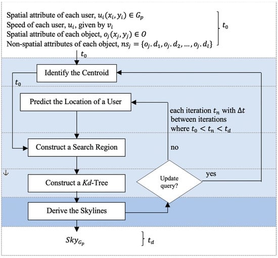
Figure 2.
The Region-based Skyline for a Group of Mobile Users (RSGMU) method.
4.1. Identify the Centroid
When a group of users, , where each user, , is located at a different location, decided to meet, there must be a point to guide the direction of their movements. Is the norm to select a point in which the travelling distance of each user is almost the same to ensure the users will be able to meet on time. In this work, it was assumed that these users will move towards a point that has the tendency to be a centre based on the users′ locations. This point is called centroid and is denoted by . The centroid of a given group of users, , is determined using the following formula [32]:
where is the coordinate of user location, is the coordinate of user location, is the average of the coordinates of all users in the group , and is the average of the coordinates of all users in the group . Note that this step is performed only once with users′ locations as given at time . This step is reflected in Algorithm 1. Based on the example shown in Table 2, the centroid of is .
| Algorithm 1: Identify the Centroid |
| Input: A group of users, with each user given as |
| Output: Centroid, |
| 1. Begin |
| 2. /* Equation (1) |
| 3. End |
4.2. Predict the Location of a User
The aim of this phase is to predict the location of a user while the user is on the move. To achieve this, we utilised the dynamic motion formula proposed by [31]. Here, we assumed that each user, , is moving in a steady speed, , towards the centroid, , which was identified in the previous phase. Consequently, the location of at time given by ) changes to ) at time, , where . Intuitively, the objects that are initially the possible candidate skylines based on ), i.e., in the boundary of the user′s region, are no longer the possible candidates due to the new location of the user, i.e., ). This means skylines have to be continuously updated by discarding the irrelevant objects until an object is selected as a meeting point. Hence, predicting the values of and of each user ahead of time would assist the users to foresee the potential meeting points. In the following, we show (i) an arbitrary movement and (ii) a centroid-based movement and their effect on the objects of interest of a user.
Figure 3a shows an example of an arbitrary movement of a user, , with the location at time and a list of objects, . Based on the initial location of , let us assume that the region of interest (refer to Definition 8) of with radius is the region (shown in shaded black). The objects that fall within the region are said to be the objects of interest (refer to Definition 10) to compared to other objects that are outside of the region . Thus, objects , and are the possible objects to be visited by , while objects , , , , , , , , , , and , which are outside of the region , are the uninterested objects to . At time , where , the new location of is . Based on this new location and assuming the same radius , the region of interest of is no longer but (shown in shaded red). Here, the objects of interest to user are , , and . It is obvious that there are objects that were initially in the list of objects of interest, and , which are no longer the objects of interest based on the new location of . Additionally, there are objects that were not initially in the list of objects of interest, , and , which are now the objects of interest based on the new location of . Therefore, it is essential to predict the new location of a user at time where , as the set of objects of interest of a user might be different at different times.
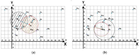
Figure 3.
(a) The regions of interest, and , when changed their location, (b) The regions of interest, and , when user moves towards .
In a centroid-based movement, it is assumed that the group of users is moving towards a centroid, . Hence, the region is a subset of the region , as clearly shown in Figure 3b. As the user becomes closer to the centroid, the search region becomes smaller. Here, the objects of interest based on , i.e., based on the initial location of user at time , are , , , and , while the objects of interest based on , i.e., based on the new location of user at time , are and . This means the objects and , which were initially the objects of interest, are now no longer the objects of interest.
Figure 4 shows a user, , with the location ) is moving towards the centroid , with the location . Let us assume that at time , the new location of is ). In order to find the values of and , the following needs to be calculated: (i) the displacement , (ii) the and , and (iii) the displacement . The detailed steps are presented below.
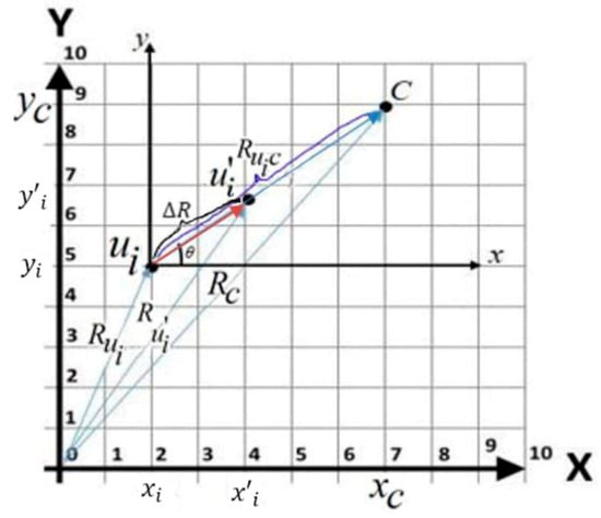
Figure 4.
The displacement when user is moving towards the centroid .
Step 1: Calculate the displacement from to . The displacements from point to and from to are presented as displacement vectors, and , respectively. The net displacement of these two displacements is a single displacement from to , which is called [31]. The equations to find the displacement are as follows:
From Equation (2), we obtained:
From Equations (3) and (4), we obtained:
Step 2: Calculate the and . This step calculates the value of , which is an angle between the positive direction of the axis and the direction of . Given the components and , the orientation of the vector is calculated as follows:
From Equation (7), we obtained:
Step 3: Calculate the displacement at time with speed . The displacement at time with speed is calculated using the following equations [31]:
Step 4: Calculate the and at time . The displacement interval is the difference between the displacements and , which were calculated in steps 1 and 3, respectively.
From Equation (8), we obtained:
From Equation (13), we obtained:
From Equation (9), we obtained:
From Equation (15), we obtained:
Based on the example shown in Table 2, Table 4 and Table 5 show the predicted locations of users , and at and with s.
Table 4.
The new locations of the users at t1.
Table 5.
The new locations of the users at t2.
The steps explained above are shown in Algorithm 2.
| Algorithm 2: Predict the Location of a User |
| Input: A group of users, with each user given as ; Centroid |
| Output: A group of users, with each user’s location being updated as ) |
| 1. Begin |
| 2. For each do |
| 3. Calculate the displacement /* Equation (7) |
| 4. Calculate the cosine and sine as follows: /* Equation (8) /* Equation (9) |
| 5. Calculate the displacement at time with speed , where /* Equation (11) |
| 6. Calculate and at time : /* Equation (14) /* Equation (16) |
| 7. End |
| 8. End |
4.3. Construct a Search Region
The aim of constructing a search region (Refer to Definition 9) is to limit the searching space to those spaces in which the objects of interest can be easily identified and, consequently, the skyline objects can be located. Given users in a group, the objects of interest are those objects that are within the regions of interest of these users. This is achieved by: (1) identifying the search region for each user, , and (ii) identifying the search region given a group of users, .
4.3.1. Identify the Search Region for Each User,
In the case where no object is found at the centroid identified in the previous step, the nearest object,, to the centroid has to be determined. The nearest object is an object with the shortest Euclidean distance from the centroid. Based on the example shown in Table 2, the nearest object is (3.2, 4). The search region for a user, , denoted as , is the area bound by a circle with radius . The radius of is determined by a straight line from to , i.e., a straight line from ) to ). However, the nearest object can also be at the point , i.e., . Figure 5 shows the construction of a search region for user,, where (a) the nearest object is nearer to the user compared to , (b) the nearest object is further from the user compared to , and (c) the nearest object is at the same point as . The further the user is from the nearest object , the larger the search region of , , is. Figure 6a presents the search regions of three users, and . It is obvious that the areas covered are different in sizes with user having the largest search region than and since the distance between and is the furthest compared to the distances of and to .
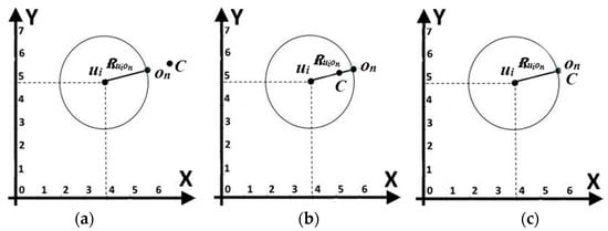
Figure 5.
The search region of user ui: (a) the nearest object on is nearer to the user ui compared to C, (b) the nearest object on is further from the user ui compared to C, and (c) the nearest object on is at the same point as C.
4.3.2. Identify the Search Region Given a Group of Users, SG
This step is simply achieved by performing union on the search region of each user in the group, i.e., . The shaded area in Figure 6a presents the search region for a group of users, SG, which is derived as follows: SG = .

Figure 6.
(a) The search region for a group of users. (b) The general region, , with radius .
4.4. Construct a Kd-Tree
The changes in the users′ locations of a group at time, , caused the search region of the group , built at time in the previous phase, to be reconstructed, where . In this work, the changes are captured at a certain time interval, which is assumed to be specified by the users. With the centroid-based movement, the search region, , constructed at time is a subset of , constructed at time This implies that the objects of interest of are a subset of the objects of interest of . Undoubtedly, it is unwise to scan the whole objects at every time interval, i.e., , until a skyline object is selected as a meeting point at time . Moreover, due to the objects of interest at every iteration being a subset of objects of interest of the preceding iterations, these objects should be organised in such a way that the uninterested objects in each iteration can be easily identified and filtered out from this collection of objects. To achieve the above, we utilised the Kd-tree. The steps taken in constructing a Kd-tree are: (1) identify the general region of a group of users, (2) construct a minimum bounding rectangle (MBR) based on the general region identified in step (1), and (3) build a Kd-tree based on the MBR that was constructed in step (2). These steps are further clarified in the following subsections.
4.4.1. Identify the General Region of a Group of Users
In order to construct a Kd-tree, a region must be defined. The objects that fall within the region are inserted in the Kd-tree. Here, the region is called general region, , and it is determined by: (1) identifying the farthest user, , from the nearest object , i.e., (2) identifying the radius of the general region by multiplying the radius with 2 (the diameter of ) where is a straight line from to , i.e., a straight line from ) to ); and (3) drawing a circle that represents the general region with as the radius and as the center point. Figure 6b shows an example of a general region with radius .
4.4.2. Construct a Minimum Bounding Rectangle (MBR) Based on the General Region
Before the Kd-tree can be constructed, a minimum bounding rectangle (MBR) should be identified. There are two types of MBR, namely, single minimum bounding rectangle (SMBR) and multiple minimum bounding rectangle (MMBR). In the SMBR, only a single MBR is constructed for all users in the group with a length and width of the MBR equal to the diameter of . Meanwhile, in MMBR, a MBR is constructed for each user, , with a length and width of each MBR equal to the diameter of . Figure 7a,b show a sample of SMBR and MMBR, respectively.
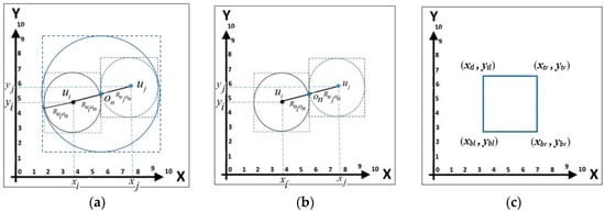
Figure 7.
(a) Single minimum bounding Rectangle (SMBR). (b) Multiple minimum bounding rectangle (MMBR). (c) Minimum bounding rectangle (MBR).
The following notations are used when referring to a MBR: : the coordinate at the bottom left of the MBR; : the coordinate at the bottom right of the MBR; : the coordinate at the top left of the MBR; and : the coordinate at the top right of the MBR. Figure 7c depicts these notations.
The following discusses the construction of SMBR and MMBR. Consider a user, ), the nearest object, ), radius, , and (i.e., ). The vertexes of the SMBR are calculated as follows: ; ; ; ; ; ; , and . If there are users, only one MBR needs to be constructed. Meanwhile, the vertexes of the MMBR are calculated as follows: ; ; ; ; ; ; ; and . If there are users, then MBRs need to be constructed.
Table 6.
Example of the calculation of SMBR.
Table 7.
Example of the calculation of MMBR.
Based on the examples shown in Table 6 and Table 7, the SMBR and MMBR are as shown in Figure 8. From this figure, the following can be observed:
- (i)
- In calculating the coordinates of a MBR, eight operations as described above need to be performed, i.e., , , , , , , , and . The calculation of the coordinates of the MBR for MMBR requires operations, while for SMBR only eight operations are needed.
- (ii)
- The MMBR is a subset of SMBR and thus the objects that fall within the area of MMBR are also the objects that fall within the area of SMBR but not vice versa. As such, the number of objects covered by MMBR is lesser than those covered by SMBR.
- (iii)
- Both MMBR and SMBR might contain uninterested objects; however, the number of uninterested objects in MMBR is lesser than or equal to the number of uninterested objects in SMBR.

4.4.3. Build a Kd-Tree Based on the MBR
Once the MBR is identified, a Kd-tree is constructed, in which objects that fall within the boundary of the MBR are inserted into the Kd-tree. Figure 9a,b show the Kd-trees constructed based on SMBR and MMBR, respectively.
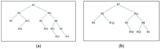
Figure 9.
The Kd-tree for objects that fall within (a) SMBR and (b) MMBR.
Since the Kd-tree constructed for SMBR and MMBR is based on the general region and search region of individual user, respectively, uninterested objects might be among the elements of the tree. The shaded area in Figure 10 is the area where the uninterested objects might fall. Based on this example, objects , , , , and are the uninterested objects. The common uninterested objects for both SMBR and MMBR are , , and .
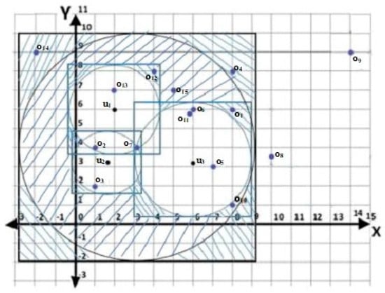
Figure 10.
The objects within the SMBR and MMBR.
The Kd-tree is traversed to identify the objects that fall within the search region of the group of users, i.e., the objects of interest to the group of users. In general, any objects that fall within the search region of an individual user are the objects of interest to the group of users. In order to achieve this, the following steps are performed:
- (1)
- Traverse the Kd-tree in a depth first traversal manner.
- (2)
- For each visited object in the Kd-tree, , if the object falls within the region of any search region of an individual user, , then the object is considered as one of the objects of interest for the group of users. There are three possible cases based on the location of an object and its relevance position to a search region. These cases are as follows:
- (a)
- The object is outside the search region of an individual user, . Here, if the Euclidean distance between the object and the user is greater than the radius of the search region, , then is said to be outside the boundary of . This condition is written as , .
- (b)
- The object falls within the search region of an individual user, . Here, if the Euclidean distance between the object and the user is less than the radius of the search region, , then is said to be within the boundary of . This condition is written as , .
- (c)
- The object intersects with the boundary of a search region of an individual user, . Here, if the Euclidean distance between the object and the user is equal to the radius of the search region, , then is said to intersect with the boundary of . This condition is written as , .
The objects that satisfy cases (b) or (c) are the objects of interest to the group of users. The notation is used to denote this set of objects, while objects that satisfy case (a) are the uninterested objects. Algorithm 3 shows the detail steps as elaborated in this section.
| Algorithm 3: Construct a Kd-tree Algorithm |
| Input: A group of users, with each user given as A set of objects ; The nearest object to , ; A search region of each user with radius |
| Output: A list of objects of interest, |
| 1. Begin |
| 2. |
| 3. For each do |
| 4. Obtain the Euclidean distance between |
| 5. End |
| 6. Obtain the farthest user, , from , where |
| 7. Identify the radius of the general region |
| 8. Construct the general region area bound by a circle with radius and as the center point |
| 9. Construct an with the following vertices: ; ; ; ; ; ; , and |
| 10. For each do |
| 11. If is within the , then insert into the Kd-tree |
| 12. End |
| 13. Obtain the object of interest, , by traversing the Kd-tree: If , or , , then |
| 14. End |
We conducted two simple analyses to confirm that having a single MBR (SMBR) is better than constructing a MBR for each user, i.e., MMBR. Figure 11a shows the results of processing time required in constructing a SMBR compared to MMBR. In this analysis, the TIGER dataset with 50 restaurants in [0, 1000]*[0, 1000] space was utilised, while the number of users varied from 1 to 30. These users were randomly selected from the TIGER dataset. The results show that the processing time of SMBR is always 0.018 s regardless the number of users, while the processing time of MMBR increases when the number of users increases. Meanwhile, Figure 11b shows the results of the second analysis that described the processing time required when the whole process presented in this section is performed, i.e., construct the MBR and build as well as traverse the Kd-tree. The same dataset was used with 16 users in [0, 1000]*[0, 1000] space. The number of objects varied from 50 to 150. These objects were randomly selected from the dataset. The results clearly show that the processing time increases when the number of objects increases; however, the processing time of SMBR is lower than the processing time of MMBR. Based on these analyses, SMBR was utilised in this work.
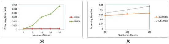
Figure 11.
The processing time of (a) SMBR and (b) MMBR.
4.5. Derive the Skylines
This step derives and updates the skyline objects,, for a group of users, , at a specified time interval, . The skyline objects were derived by considering both the spatial and non-spatial attributes of the objects of interest, , identified in Section 4.4 as well as the spatial attribute of the user. The value of the spatial attribute of a user at time is the initial location of the user , given by ), while at time , where , the value is as predicted at time and denoted by ). Hence, in order to derive , both and need to be identified, where reflects those objects of that non-spatially dominate the other objects, while represents those objects of that spatially dominate the other objects. Here, the Definition 4. Non-spatial Dominance, Definition 5. Spatial Dominance, Definition 6. Dominance in a Space, and Definition 7. Skylines of a Space, defined in Section 3, are important. The detail steps are presented in Algorithm 4.
4.5.1. Derive the Spatial Skylines
This step applies the spatial dominance testing provided in Definition 5. Spatial Dominance towards the list. First, the distance between each object, , and each user, , is determined, denoted as . Given a group of users, there will be values of distances with regard to the object , i.e., . These values are treated as the values of dimensions to be used in the spatial skyline computation. Then, the total distance between an object, , to each user, , in the group of users is calculated and saved into a parameter named , i.e., . The value of is used as a selection criterion in determining the object that should be considered in each iteration of the spatial skyline computation. The smallest value of indirectly indicates that most users in the group are close to the object and has more chances to dominate the other objects. An example is shown in Table 8. In the table, the columns , and are the distances of each object, , and each user , and , respectively, while the column in the table presents the total distance of an object to each user in the group of users. In this example, it is assumed that , , , , , , and the locations of each user are as predicted at time with s.
Table 8.
Spatial attributes of objects at time .
Based on Table 8, the object with the lowest , i.e., with was selected and compared to the other objects of . Using the Definition 5. Spatial Dominance, . The dominated object, , was removed from the list and the same process was repeated with the remained objects in . Based on the example provided, .
4.5.2. Derive the Non-Spatial Skylines
To derive , the Definition 4. Non-spatial Dominance was used. The list of objects of interest, , identified in Section 4.4 was again analysed; however, in this step, the analysis was based on the non-spatial attributes of the objects. Based on the given and the non-spatial attributes , since , , , , and .
4.5.3. Derive the Final Skylines
The final skyline objects, , for the group of users, , at time is given by . For the above example, .
| Algorithm 4: Derive the Skylines Algorithm |
| Input: A list of objects of interest, ; A group of users, |
| Output: Final skylines, |
| 1. Begin |
| 2. Let |
| 3. For each do |
| 4. For each do |
| 5. If then /* Definition 4 |
| 6. Else If then /* Definition 4 |
| 7. End |
| 8. End |
| 9 |
| 10. Let |
| 11. For each do |
| 12. For each do |
| 13. Get the distance between and |
| 14. End |
| 15. |
| 16. End |
| 17. Sort the objects of based on the in ascending order |
| 18. For each do |
| 19. For each do |
| 20. If then /* Definition 5 |
| 21. Else If then /* Definition 5 |
| 22. End |
| 23. End |
| 24. |
| 25. /* Definition 7 |
| 26. End |
5. Results and Discussion
We designed and conducted several extensive experiments in an attempt to fairly evaluate the performance and prove the efficiency of RSGMU. The implementation of RSGMU was performed on VB.NET 2013, while the experiments were conducted on Intel Core i7 3.6 GHz processor with 32 GB of RAM and Windows 8 professional. Each experiment was run 10 times and the average value with regard to processing time of these runs was reported. The performance results of RSGMU were compared to those of the VR algorithm proposed by [28]. Although the work in [4] focused on continuous query, only the spatial attribute of the user and the objects were analysed in deriving the skyline objects, i.e., no performance results were reported in [4], in which both spatial and non-spatial attributes of the objects were considered in the skyline computation. Meanwhile, two types of datasets were used in the experiments, namely, synthetic and TIGER datasets. The TIGER dataset is a real dataset commonly used in the spatial skyline queries [4,5,28]. The dominated objects are derived based on the assumption that lower values are preferable compared to higher ones. The parameter settings are shown in Table 9, with values in bold representing the default values. The performance results of RSGMU and the VR algorithm were reported based on these parameter settings in the following paragraphs.
Table 9.
The parameter settings of the synthetic and TIGER datasets.
Effect of Time Interval,: The main aim of this experiment is to investigate the effect of time interval, , on the performance of RSGMU. In this experiment, the parameter settings for the synthetic dataset were as follows: the time interval varied with the following values: 10 s, 20 s, 30 s and 40 s; the number of dimensions was set to six dimensions and the number of users in a group was 15 in [0, 1000]*[0, 1000], while the number of objects was set to 50 K. For the TIGER dataset, the same parameter settings as above were used, except that the number of objects was maintained at its initial number, i.e., 50,747 objects, with the number of dimensions being fixed to 2. Figure 12 presents the number of skyline objects and number of objects of interest for each time interval for both datasets, synthetic and TIGER. At time , the number of skyline objects and the number of objects of interest for all time intervals are the same. This is because, in each run, the search region constructed for the group of users is based on the initial location of each user. Hence, each deals with the same set of objects of interest and consequently derive the same set of skyline objects. This is as shown in Figure 12a–d at Iteration 1. Nonetheless, the number of iterations for each time interval differs; for instance, the average number of iterations when s is 35, while s took 11 iterations to reach . Here, is the final state when one of the users has reached the nearest object, , to the centroid (see Section 4.3.1). Undeniably, the smaller the , the more iterations are performed with little difference in the number of objects of interest and skyline objects between iterations. Nevertheless, the final state of each indicates that all produce the same number of skyline objects. Based on this experiment, we decided to use s in the subsequent experiments to ensure that objects in the space were rigorously explored. Moreover, to avoid bias in the comparisons, the with the longest time (highest number of iterations) to reach was chosen.
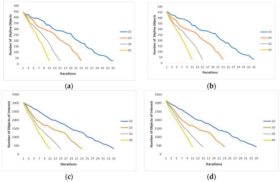
Figure 12.
The results of number of skyline objects and number of objects of interest with varying time intervals. (a) Synthetic. (b) TIGER. (c) Synthetic. (d) TIGER.
Effect of Number of Objects: The parameter settings for the synthetic dataset in this experiment were as follows: the number of dimensions was fixed to six and the number of users in a group was 15 in [0, 1000]*[0, 1000], while the number of objects varied with the following values: 20 K, 50 K and 80 K. Since the TIGER dataset contains only 50,747 objects, it was excluded from this experiment. Figure 13 presents the processing time gained by the RSGMU and the VR algorithm [28] based on the synthetic dataset. Intuitively, when the number of objects increases, the processing time also increases. From the figure, it is obvious that the number of objects has a significant impact on the performance of both the RSGMU and the VR algorithm. Nevertheless, RSGMU was better than the VR algorithm in all the runs. This is because, the VR algorithm constructs both the Voronoi and R-Tree based on the objects of the entire dataset. These structures are then traversed to identify those objects that fall within the search region of the users that is derived based on their current locations. This means that, whenever the users′ locations changed, the whole structures have to be traversed to identify the objects that are within the new search region of the users. Meanwhile, RSGMU constructs a Kd-tree based on the objects that fall within the search region of the users. Hence, objects that are not within the search region are removed from being analysed as early as possible. When the users′ locations changed, the Kd-tree is traversed and updated to reduce unnecessary computation. As a result, RSGMU managed to reduce the processing time significantly with an average of 35% improvement compared to the VR algorithm.
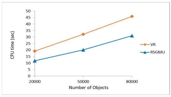
Figure 13.
The results of processing time with varying number of objects.
Effect of Data Dimensionality: In this experiment, the parameter settings for the synthetic dataset were as follows: the number of dimensions varied from 2 to 10 dimensions and the number of users in a group was 15 in [0, 1000]*[0, 1000], while the number of objects was set to 50 K. For the TIGER dataset, the same parameter settings as above were used, except that the number of objects was maintained to its initial number, i.e., 50,747 objects in [0, 1000]*[0, 1000]. The comparison of the results of processing time presented in Figure 14a,b reveals that the performance of RSGMU is better than the performance of VR algorithm for both the synthetic and TIGER datasets. In fact, RSGMU shows a steady performance even when the number of dimensions is increased, while a slight increment in processing time can be seen in the VR algorithm. The same reasons provided earlier apply here. The RSGMU gained improvements with regard to processing time with an average of 44% and 45% for the synthetic and TIGER datasets, respectively, as compared to the VR algorithm.
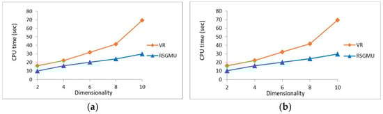
Figure 14.
The results of processing time with varying dimensionality. (a) Synthetic. (b) TIGER.
Effect of Density: This experiment, which aims at investigating the effect of density on the performance of the proposed method, utilised only the TIGER dataset. This is due to the fact that the TIGER dataset contains eight distinct types of objects as listed in Table 10, with each type having a certain number of objects as shown by the No. of objects column of the table. The density rate was derived by simply dividing the No. of objects with the whole population. Thus, the % of the type of object in the whole population reflects the density rate of a particular type of object in the area. For instance, the density rates of hospital and institution are and , respectively. From Table 10, it is observed that institution is the densest objects.
Table 10.
The density rate of the types of objects in the TIGER dataset.
The parameter settings for this experiment were as follows: the number of objects was 50,747, the number of users in a group was 15 in [0, 1000]*[0, 1000], and the number of dimensions was fixed to two. The density rates used were as follows: 0.56% (hospital), 1.60% (restaurant), 7% (church), 15% (school), and 34% (institution). From Figure 15, it is obvious that the higher the density rate, the higher is the processing time. The performance of RSGMU and the VR algorithm shows similar trends in which it starts to show a drastic increment when the density rate is 15% until it reaches 34%. This is due to the fact that the number of institutions (34%) is slightly more than twice the number of schools (15%). Nonetheless, the percentage of improvement gained by RSGMU is 12% compared to the VR algorithm.
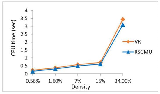
Figure 15.
The results of processing time with varying density.
Effect of Space Size: The parameter settings used in this experiment for the TIGER dataset were as follows: the number of objects was fixed to 50,747 objects, the number of users in a group was 15, and the number of dimensions was set to two. For the synthetic dataset, the same parameter settings as above were used, except that the number of objects was set to 50 K objects. For both datasets, the space size varied as follows: [0, 250]*[0, 250], [0, 500]*[0, 500], [0, 750]*[0, 750], and [0, 1000]*[0, 1000]. From Figure 16, it is evident that, when the space size increases, the processing time also increases, as reflected in the results of both solutions. Nonetheless, RSGMU achieved better performance as compared to VR and managed to reduce the processing time significantly with an average of 37% and 42% improvement for the synthetic and TIGER datasets, respectively.
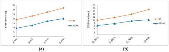
Figure 16.
The results of processing time with varying space size. (a) Synthetic. (b) TIGER.
Effect of Number of Users in a Group: In this experiment, the number of mobile users in a group varied in the range of 4–25, while the parameter settings for the synthetic dataset were as follows: the number of objects was fixed to 50 K and the space was fixed to [0, 1000]*[0, 1000], while the number of dimensions was set to 6. For the TIGER dataset, the same parameter settings as above were used, except that the number of objects was maintained at its initial number, i.e., 50,747 objects, with the number of dimensions being fixed to two. From Figure 17a,b, it is evident that both RSGMU and the VR algorithm show a steady increase in the processing time, which reflects that the number of users in a group has an impact on the performance of both solutions. However, RSGMU achieved a better performance as compared to VR with an average of 36% improvement for the synthetic dataset and 38% for the TIGER dataset, since unnecessary skyline computations were avoided by organising only those objects that fall within the search region of the users in a Kd-tree.
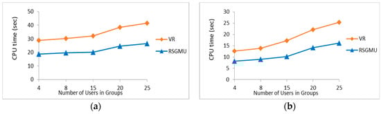
Figure 17.
The results of processing time with varying number of users in a group. (a) Synthetic. (b) TIGER.
Effect of Number of Groups of Users: In this experiment, the parameter settings for the synthetic dataset were as follows: the number of objects was fixed to 50 K, the number of users in each group was set to 15, and the number of dimensions was fixed to six. For the TIGER dataset, the same parameter settings as above were used, except that the number of objects was maintained at its initial number, i.e., 50,747 objects in [0, 1000]*[0, 1000], with the number of dimensions being fixed to two. Meanwhile, the number of groups of users varied from 2 to 32 groups for both datasets. Figure 18a,b present the processing time achieved by the RSGMU and VR algorithm [28], based on the synthetic and TIGER datasets, respectively. From these figures, RSGMU shows a steady performance, which reflects that there is a slight increment in the processing time in each run due to the increment in the number of groups of users. The same trend is true for the performance of the VR algorithm. Nonetheless, RSGMU achieved a better performance compared to VR with an average of 36% and 41% improvements for the synthetic and TIGER datasets, respectively.
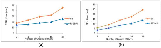
Figure 18.
The results of processing time with varying number of groups of users. (a) Synthetic. (b) TIGER.
Number of Skyline Objects: In this experiment, the correctness of RSGMU was validated by comparing the skyline objects derived by RSGMU against those skyline objects produced by the VR algorithm. The parameter settings for the synthetic dataset were as follows: the number of objects was fixed to 50 K, the space was set to [0, 1000]*[0, 1000] and the number of dimensions was fixed to six, while the number of users in a group varied in the range of 4–25. For the TIGER dataset, the same parameter settings as above were used, except that the number of objects was maintained at its initial number, i.e., 50,747 objects, with the number of dimensions being fixed to two. From Figure 19a,b, it is evident that the number of skyline objects derived by RSGMU is the same number of skyline objects produced by the VR algorithm in all the runs; hence, the correctness of RSGMU was verified.
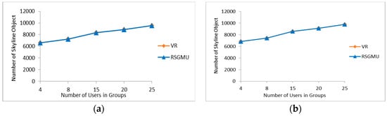
Figure 19.
The results of number of skyline objects under different number of users in a group. (a) Synthetic. (b) TIGER.
6. Conclusions
This paper presented the Region-based Skyline for a Group of Mobile Users (RSGMU) method, which aims to continuously find the optimal meeting or gathering points for a group of users while they are on the move. RSGMU consists of five steps, namely: (1) Identify the centroid, (2) Predict the location of a user, (3) Construct a search region, (4) Construct a Kd-tree, and (5) Derive the skylines. These steps are repeated in several iterations until a skyline object is selected as a meeting or gathering point. RSGMU assumes a centroid-based movement where users are assumed to be moving towards a centroid. Unlike previous works that require users to frequently report their latest locations, RSGMU utilises the dynamic motion formula to predict the locations of the users at a specified time interval, which results in the skyline objects to be continuously updated. Moreover, the skyline results can be derived ahead of time in order to assist the users to foresee the potential meeting points. Furthermore, to avoid the recomputation of skylines at each time interval, the objects of interest that are within a single minimum bounding rectangle that is formed based on the current search region are organized in a Kd-tree data structure. Several experiments with various parameter settings were conducted and the results show that our proposed method outperforms previous work with respect to CPU time.
Further enhancement that can be achieved towards the work presented in this paper includes considering asymmetric objects, i.e., objects having different properties. Most works assumed all objects in the collection have identical features, such as rating and price; however, considering and suggesting asymmetric objects as meeting or gathering points can provide more insight to the users. This means that the collection of objects contains different classes of objects with each class of objects having different properties. Skyline objects can be derived based on these different classes of objects.
Author Contributions
Conceptualization, G.B.D., H.I., F.S. and N.I.U.; methodology, G.B.D. and H.I.; validation, G.B.D., H.I. and A.A.A.; formal analysis, G.B.D., H.I., F.S. and N.I.U.; investigation, G.B.D., H.I., F.S., N.I.U., A.A.A. and M.M.L.; resources, G.B.D. and H.I.; writing—original draft preparation, G.B.D. and H.I.; writing—review and editing, H.I., F.S., N.I.U., A.A.A. and M.M.L.; visualization, G.B.D. and H.I.; supervision, H.I., F.S., N.I.U. and A.A.A.; project administration, H.I.; funding acquisition, H.I. All authors have read and agreed to the published version of the manuscript.
Funding
This work was supported by the Ministry of Higher Education Malaysia under the Fundamental Research Grant Scheme (FRGS/1/2020/ICT03/UPM/01/1) and the Universiti Putra Malaysia. All opinions, findings, conclusions and recommendations in this paper are those of the authors and do not necessarily reflect the views of the funding agencies. We thank the anonymous reviewers for their comments.
Data Availability Statement
Not applicable.
Acknowledgments
The authors would like to thank the Ministry of Higher Education Malaysia and the Universiti Putra Malaysia for funding this research work.
Conflicts of Interest
The authors declare no conflict of interest.
References
- Börzsönyi, S.; Kossmann, D.; Stocker, K. The Skyline Operator. In Proceedings of the 17th International Conference on Data Engineering, Washington, DC, USA, 2–6 April 2001; pp. 421–430. [Google Scholar]
- Dehaki, G.B.; Ibrahim, H.; Udzir, N.I.; Sidi, F.; Alwan, A.A. A Framework for Processing Skyline Queries for a Group of Mobile Users. In Proceedings of the 20th International Conference on Information Integration and Web–based Applications & Services, Yogyakarta, Indonesia, 19–21 November 2018; pp. 333–339. [Google Scholar]
- Fu, X.; Miao, X.; Xu, J.; Gao, Y. Continuous Range–based Skyline Queries in Road Networks. J. World Wide Web 2017, 20, 1443–1467. [Google Scholar] [CrossRef]
- Sharifzadeh, M.; Shahabi, C. The Spatial Skyline Queries. In Proceedings of the 32nd International Conference on Very Large Data Bases, Seoul, Korea, 12–15 September 2006; pp. 751–762. [Google Scholar]
- Sharifzadeh, M.; Shahabi, C.; Kazemi, L. Processing Spatial Skyline Queries in Both Vector Spaces and Spatial Network Databases. J. ACM Trans. Database Syst. 2009, 34, 1–45. [Google Scholar] [CrossRef]
- Sharifzadeh, M.; Shahabi, C. Vor–tree: R–trees with Voronoi Diagrams for Efficient Processing of Spatial Nearest Neighbor Queries. In Proceedings of the International Conference on Very Large Data Bases, Singapore, 13–17 September 2010; pp. 1231–1242. [Google Scholar]
- Cai, Z.; Cui, X.; Su, X.; Guo, L.; Ding, Z. Speed and Direction Aware Skyline Query for Moving Objects. J. IEEE Trans. Intell. Transp. Syst. 2020, 23, 301–312. [Google Scholar] [CrossRef]
- Huang, Z.; Lu, H.; Ooi, B.C.; Tung, A.K. Continuous Skyline Queries for Moving Objects. J. IEEE Trans. Knowl. Data Eng. 2006, 18, 1645–1658. [Google Scholar] [CrossRef]
- Lin, X.; Xu, J.; Hu, H. Range–based Skyline Queries in Mobile Environments. J. IEEE Trans. Knowl. Data Eng. 2011, 25, 835–849. [Google Scholar] [CrossRef]
- Lin, X.; Xu, J.; Hu, H.; Lee, W.C. Authenticating Location–based Skyline Queries in Arbitrary Subspaces. J. IEEE Trans. Knowl. Data Eng. 2013, 26, 1479–1493. [Google Scholar] [CrossRef]
- Tan, K.L.; Eng, P.K.; Ooi, B.C. Efficient Progressive Skyline Computation. In Proceedings of the International Conference on Very Large Databases, Roma, Italy, 11–14 September 2001; pp. 301–310. [Google Scholar]
- Kossmann, D.; Ramsak, F.; Rost, S. Shooting Stars in the Sky: An Online Algorithm for Skyline Queries. In Proceedings of the 28th International Conference on Very Large Databases, Hong Kong, China, 20–23 August 2002; pp. 275–286. [Google Scholar]
- Papadias, D.; Tao, Y.; Fu, G.; Seeger, B. An Optimal and Progressive Algorithm for Skyline Queries. In Proceedings of the ACM International Conference on Management of Data, San Diego, CA, USA, 10–12 June 2003; pp. 467–478. [Google Scholar]
- Chomicki, J.; Godfrey, P.; Gryz, J.; Liang, D. Skyline with Presorting. In Proceedings of the 19th International Conference on Data Engineering, Bangalore, India, 5–8 March 2003; pp. 717–816. [Google Scholar]
- Godfrey, P.; Shipley, R.; Gryz, J. Maximal Vector Computation in Large Data Sets. In Proceedings of the 31th International Conference on Very Large Data Bases, Trondheim, Norway, 30 August–2 September 2005; pp. 229–240. [Google Scholar]
- Bartolini, I.; Ciaccia, P.; Patella, M. SaLSa: Computing the Skyline without Scanning the Whole Sky. In Proceedings of the 15th ACM International Conference on Information and Knowledge Management, Kansas City, VA, USA, 6–11 November 2006; pp. 405–414. [Google Scholar]
- Kalyvas, C.T. A Survey of Skyline Query Processing. 2017. Available online: https://arxiv.org/pdf/1704.01788.pdf (accessed on 3 March 2018).
- Khalefa, M.E.; Mokbel, M.F.; Levandoski, J.J. Skyline query processing for uncertain data. In Proceedings of the 19th ACM International Conference on Information and Knowledge Management, Toronto, Canada, 26–30 October 2010; pp. 1293–1296. [Google Scholar]
- Alwan, A.A.; Ibrahim, H.; Udzir, N.I.; Sidi, F. An Efficient Approach for Processing Skyline Queries in Incomplete Multidimensional Database. Arab. J. Sci. Eng. 2016, 41, 2927–2943. [Google Scholar] [CrossRef]
- Gulzar, Y.; Alwan, A.A.; Turaev, S. Optimizing Skyline Query Processing in Incomplete Data. J. IEEE Access 2019, 7, 178121–178138. [Google Scholar] [CrossRef]
- Gulzar, Y.; Alwan, A.A.; Salleh, N.; Al Shaikhli, I.F. Processing Skyline Queries in Incomplete Database: Issues, Challenges and Future Trends. J. Comput. Sci. 2017, 13, 647–658. [Google Scholar] [CrossRef][Green Version]
- Dehaki, G.B.; Ibrahim, H.; Sidi, F.; Udzir, N.I.; Alwan, A.A.; Gulzar, Y. Efficient Computation of Skyline Queries over a Dynamic and Incomplete Database. J. IEEE Access 2020, 8, 141523–141546. [Google Scholar] [CrossRef]
- Dehaki, G.B.; Ibrahim, H.; Alwan, A.A.; Sidi, F.; Udzir, N.I. Efficient Skyline Computation over an Incomplete Database with Changing States and Structures. J. IEEE Access 2021, 9, 88699–88723. [Google Scholar] [CrossRef]
- Li, X.; Wang, Y.; Li, X.; Wang, G. Skyline query processing on interval uncertain data. In Proceedings of the 15th International Symposium on Object/Component/Service–Oriented Real–Time Distributed Computing Workshops, Shenzhen, China, 11–13 April 2012; pp. 87–92. [Google Scholar]
- Saad, N.H.M.; Ibrahim, H.; Sidi, F.; Yaakob, R.; Alwan, A.A. Efficient Skyline Computation on Uncertain Dimensions. J. IEEE Access 2021, 9, 96975–96994. [Google Scholar] [CrossRef]
- Lawal, M.A.M.; Ibrahim, H.; Mohd Sani, N.F.; Yaakob, R. An Indexed Non–probability Skyline Query Processing Framework for Uncertain Data. In Proceedings of the International Conference on Advanced Machine Learning Technologies and Applications, Jaipur, India, 13–15 February 2020; pp. 289–301. [Google Scholar]
- Geng, M.; Arefin, M.S.; Morimoto, Y. A Spatial Skyline Query for a Group of Users Having Different Positions. In Proceedings of the 3rd International Conference on Networking and Computing, Okinawa, Japan, 5–7 December 2012; pp. 137–142. [Google Scholar]
- Arefin, M.S.; Ma, G.; Morimoto, Y. A Spatial Skyline Query for a Group of Users. J. Softw. 2014, 9, 2938–2947. [Google Scholar] [CrossRef]
- Elmi, S.; Min, J.K. Spatial Skyline Queries over Incomplete Data for Smart Cities. J. Syst. Archit. 2018, 90, 1–14. [Google Scholar] [CrossRef]
- Dehaki, G.B.; Ibrahim, H.; Udzir, N.I.; Sidi, F.; Alwan, A.A. A Fragmentation Region–based Skyline Computation Framework for a Group of Users. In Proceedings of the International Conference on the Computer Science and Information Technology, Copenhagen, Denmark, 18–19 September 2021; pp. 35–50. [Google Scholar]
- Halliday, D.; Resnick, R.; Walker, J. Fundamentals of Physics; John Wiley & Sons: Hoboken, NJ, USA, 2013. [Google Scholar]
- Halliday, D.; Resnick, R. Physics for Students of Science and Engineering. Am. J. Phys. 1961, 29, 717–719. [Google Scholar] [CrossRef]
Publisher’s Note: MDPI stays neutral with regard to jurisdictional claims in published maps and institutional affiliations. |
© 2022 by the authors. Licensee MDPI, Basel, Switzerland. This article is an open access article distributed under the terms and conditions of the Creative Commons Attribution (CC BY) license (https://creativecommons.org/licenses/by/4.0/).