Article

Variable Matrix-Type Step-Size Affine Projection Sign Algorithm for System Identification in the Presence of Impulsive Noise

1
The Division of Electrical Engineering, Kumoh National Institute of Technology, Gumi 39177, Korea
2
The Division of Electrical Engineering, Department of IT Convergence Engineering, Kumoh National Institute of Technology, Gumi 39177, Korea
3
Department of Automobile and IT Convergence, Kookmin University, Seoul 02707, Korea
*
Author to whom correspondence should be addressed.
Symmetry 2022, 14(10), 1985; https://doi.org/10.3390/sym14101985
Submission received: 30 August 2022 / Revised: 20 September 2022 / Accepted: 20 September 2022 / Published: 22 September 2022
(This article belongs to the Special Issue Adaptive Filtering and Machine Learning)

Abstract

:
This paper presents a novel variable matrix-type step-size affine projection sign algorithm (VMSS-APSA) characterized by robustness against impulsive noise. To mathematically derive a matrix-type step size, VMSS-APSA utilizes mean-square deviation (MSD) for the modified version of the original APSA. Accurately establishing the MSD of APSA is impossible. Therefore, the proposed VMSS-APSA derives the upper bound of the MSD using the upper bound of the L 1 -norm of the measurement noise. The optimal matrix-type step size is calculated at each iteration by minimizing the upper bound of the MSD, thereby improving the filter performance in terms of convergence rate and steady-state estimation error. Because a novel cost function of the proposed VMSS-APSA was designed to maintain a form similar to the original APSA, they have symmetric characteristics. Simulation results demonstrate that the proposed VMSS-APSA improves filter performance in a system-identification scenario in the presence of impulsive noise.

1. Introduction

Adaptive-filtering theory has been researched for several decades because it can serve as a useful tool in various applications, including system identification, channel estimation, noise cancellation, acoustic echo cancellation, and network echo cancellation [1,2,3,4,5,6,7,8,9,10,11]. The least-mean-squares (LMS) and normalized LMS algorithms are representative adaptive-filtering algorithms due to their easy implementation and low computational complexity. Moreover, the affine projection algorithm (APA) [12,13,14] was suggested to improve the convergence performance of the above-mentioned algorithms for correlated input signals called colored input signals. However, the LMS-type and APA-type algorithms use L 2 -norm optimization; therefore, they have performance degradation when system output noise includes impulsive noise.
There are many kinds of adaptive-filtering algorithms that were recently proposed to achieve robustness against impulsive noise as can be shown in Figure 1 [15,16,17,18,19,20,21,22,23,24,25,26]. Unfortunately, since these adaptive-filtering algorithms use the L 1 -norm optimization, they have a slow convergence rate. To overcome this convergence-rate drawback, the affine projection sign algorithm (APSA) [16] was suggested for accomplishing a rapid convergence rate. APSA also uses the L 1 -norm optimization approach, but has a fast convergence rate owing to multiple input vectors and its specific constraint.
On the other hand, there are many studies on step-size adjustment for adaptive-filtering algorithms [20,21,22,23,24,25,26,27]. It is clear that a large step results in fast convergence, but has a large steady-state estimation error, and a small step leads to slow convergence and a small steady-state estimation error. This trade-off between the convergence rate and steady-state estimation error is obvious with APSA; therefore, a variable-step-size method is efficient in guaranteeing a fast convergence rate with a small steady-state estimation error. Moreover, because step-size adjustment is effective in improving the filter performance of APSA-type algorithms, various strategies are available for variable-step-size APSA (VSS-APSA) [20,21].
This paper presents a new variable matrix-type step-size APSA (VMSS-APSA) to enhance filter performance in terms of convergence rate and steady-state estimation error. VMSS-APSA utilizes the mean-square deviation (MSD) of APSA to judiciously calculate a step size for APSA. The proposed VMSS-APSA derives the upper bound of the MSD using the upper bound of the L 1 -norm of the measurement noise because the MSD of APSA cannot be computed accurately. The optimal matrix-type step size is derived at every iteration by minimizing the upper bound of the MSD. The performance of the proposed VMSS-APSA is demonstrated via system-identification scenarios when impulsive noise occurs. The proposed VMSS-APSA is compared with the original APSA [16], the two existing types of VSS-APSA [20,21], and robust variable-step-size APA (RVSS-APA) [22].
The remainder of this paper is arranged as follows. Section 2 summarizes the original APSA. Section 3 presents a novel variable matrix-type step-size APSA. Section 4 presents the simulation results to validate the performance of the proposed algorithm. Lastly, Section 5 concludes this paper.

2. Original APSA

Let data d ( n ) be generated from an unknown target system:
d ( n ) = u T ( n ) w o + v ( n ) ,
where w o is an m-dimensional column vector of the target system that needs to be estimated, v ( n ) denotes the measurement noise that has variance σ v 2 , and the input data vector is u ( n ) = [ u ( n ) u ( n 1 ) u ( n m + 1 ) ] T . The input data matrix, desired output vector, a priori output error vector, and a posteriori output error vector are defined as follows:
U ( n ) = [ u ( n ) u ( n 1 ) u ( n M + 1 ) ] ,
d ( n ) = U T ( n ) w o + v ( n ) , e ( n ) = d ( n ) U T ( n ) w ^ ( n ) ,
= [ e ( n ) e ( n 1 ) e ( n M + 1 ) ] T ,
e p ( n ) = d ( n ) U T ( n ) w ^ ( n + 1 ) ,
where v ( n ) = [ v 1 ( n ) v 2 ( n ) v M ( n ) ] is a measurement-noise vector whose each component v i ( n ) for 0 < i M has zero mean and variance σ v 2 , and w ^ ( n ) is the estimate of w o at nth iteration.
The original APSA is derived from the minimization of the L 1 -norm of the a posteriori output error vector with a condition on the filter coefficient vectors as follows:
min w ^ ( n + 1 ) | | d ( n ) U T ( n ) w ^ ( n + 1 ) | | 1
subject to | | w ^ ( n + 1 ) w ^ ( n ) | | 2 2 μ 2 ,
where μ is the step size that guarantees that the filter coefficient vectors do not change suddenly. This minimization problem with a constraint (6) can be solved on the basis of Lagrangian multipliers. Therefore, the filter coefficient vector of the original APSA is represented by recursively using the following update equation [16]:
w ^ ( n + 1 ) = w ^ ( n ) + μ U ( n ) sgn ( e ( n ) ) sgn ( e T ( n ) ) U T ( n ) U ( n ) sgn ( e ( n ) ) .
where sgn ( · ) denotes the sign function, and sgn ( e ( n ) ) [ sgn ( e ( n ) ) , , sgn ( e ( n M + 1 ) ) ] T .

3. Variable Matrix-Type Step-Size APSA

3.1. Optimal Matrix-Type Step Size

The filter update equation of the original APSA (8) can be modified to adjust the matrix-type step size as follows:
w ^ ( n + 1 ) = w ^ ( n ) + U ( n ) Λ ( n ) sgn ( e ( n ) ) sgn ( e T ( n ) ) U T ( n ) U ( n ) sgn ( e ( n ) ) ,
where diagonal matrix Λ ( n ) denotes the matrix-type step size as follows:
Λ ( n ) = μ 1 ( n ) 0 0 0 μ 2 ( n ) 0 0 0 μ M ( n ) .
Although the regularization parameter is commonly adopted in the denominator of Equation (9), it was omitted to simplify the proposed analysis [13]. The proposed filter update equation of APSA (9) can be described with respect to w ˜ , where the filter-coefficient error vector is defined as w ˜ ( n ) w w ^ ( n ) , and the matrix-type step size is expressed in variable parameter Λ ( n ) as follows:
w ˜ ( n + 1 ) = w ˜ ( n ) U ( n ) Λ ( n ) sgn ( e ( n ) ) sgn ( e T ( n ) ) U T ( n ) U ( n ) sgn ( e ( n ) ) .
Equation (11) is squared, and the expectation of both sides is taken to derive the updated recursion of MSD. Accordingly, the updated recursion of MSD can be expressed as follows:
E w ˜ ( n + 1 ) 2 = E w ˜ ( n ) 2 2 E sgn e T ( n ) Λ T ( n ) U T ( n ) w ˜ ( n ) sgn ( e T ( n ) ) U T ( n ) U ( n ) sgn ( e ( n ) ) + Λ T ( n ) Λ ( n ) E ( w ˜ ( n ) 2 ) + Φ ( μ 1 ( n ) , , μ M ( n ) ) ,
where notation · denotes the L2 norm, and Φ ( μ 1 ( n ) , , μ M ( n ) ) is a function of the matrix-type step size.
To minimize the MSD of VMSS-APSA from iteration n to n + 1 , function
Φ ( μ 1 ( n ) , , μ M ( n ) ) has to be minimized by choosing the optimal step size. Φ ( μ 1 ( n ) , , μ M ( n ) ) can be described as follows:
Φ ( μ 1 ( n ) , , μ M ( n ) ) = 2 μ 1 ( n ) E sgn ( e 1 ( n ) ) ( e 1 ( n ) v 1 ( n ) ) sgn ( e T ( n ) ) U T ( n ) U ( n ) sgn ( e ( n ) ) + 2 μ M ( n ) E sgn ( e M ( n ) ) ( e M ( n ) v M ( n ) ) sgn ( e T ( n ) ) U T ( n ) U ( n ) sgn ( e ( n ) ) + μ 1 2 ( n ) + + μ M 2 ( n ) = 2 μ 1 ( n ) E | e 1 ( n ) | sgn ( e 1 ( n ) ) v 1 ( n ) sgn ( e T ( n ) ) U T ( n ) U ( n ) sgn ( e ( n ) ) + 2 μ M ( n ) E | e M ( n ) | sgn ( e M ( n ) ) v M ( n ) sgn ( e T ( n ) ) U T ( n ) U ( n ) sgn ( e ( n ) ) + μ 1 2 ( n ) + + μ M 2 ( n ) ,
where the U T ( n ) w ˜ ( n ) term can be represented through Equations (2) and () as
U T ( n ) w ˜ ( n ) = U T ( n ) w o U T ( n ) w ^ ( n ) = e ( n ) v ( n ) .
The sgn ( e i ( n ) ) v i ( n ) term cannot be calculated exactly; thus, Φ ( μ 1 ( n ) , , μ M ( n ) ) cannot be obtained directly for 0 < i M . Thus, the upper bound of sgn ( e i ( n ) ) v i ( n ) can be found using the stochastic approach as follows [24,25,26]:
s g n ( e i ( n ) ) v i ( n ) | v i ( n ) | , 0 < i M ,
Because the absolute value of | v i ( n ) | is not an exactly measurable value, | v i ( n ) | is approximated as its expectation value. Moreover, because | v i ( n ) | has the characteristic of a half-normal distribution, | v i ( n ) | can be represented as follows:
| v i ( n ) | E ( | v i ( n ) | ) = 2 π σ v .
where σ v is the standard deviation of measurement noise v i ( n ) .
On the basis of the stochastic approximation, the upper bound of function Φ ( μ 1 ( n ) , , μ M ( n ) ) can be expressed as follows:
Φ ( μ 1 ( n ) , , μ M ( n ) ) 2 μ 1 ( n ) E | e 1 ( n ) | | v 1 ( n ) | sgn ( e T ( n ) ) U T ( n ) U ( n ) sgn ( e ( n ) ) + 2 μ M ( n ) E | e M ( n ) | | v M ( n ) | sgn ( e T ( n ) ) U T ( n ) U ( n ) sgn ( e ( n ) ) + μ 1 2 ( n ) + + μ M 2 ( n ) 2 μ 1 ( n ) E | e 1 ( n ) | 2 π σ v sgn ( e T ( n ) ) U T ( n ) U ( n ) sgn ( e ( n ) ) + 2 μ M ( n ) E | e M ( n ) | 2 π σ v sgn ( e T ( n ) ) U T ( n ) U ( n ) sgn ( e ( n ) ) + μ 1 2 ( n ) + + μ M 2 ( n ) Φ u ( μ 1 ( n ) , , μ M ( n ) ) .
Step size μ i ( n ) that minimizes Φ ( μ 1 ( n ) , , μ M ( n ) ) sharply decreases the MSD value from iteration n to n + 1 . Therefore, the partial differential of (17) with respect to μ ( n ) yields
Φ ( μ 1 ( n ) , , μ M ( n ) ) μ i ( n ) = 2 μ i ( n ) E | e i ( n ) | 2 π σ v sgn ( e T ( n ) ) U T ( n ) U ( n ) sgn ( e ( n ) ) + 2 μ i ( n ) , 0 < i M .
In (18), because Φ ( μ 1 ( n ) , , μ M ( n ) ) / ( μ i ( n ) ) = 0 , the derived step size μ i ( n ) can be obtained as follows:
μ i ( n ) = E | e i ( n ) | 2 π σ v sgn ( e T ( n ) ) U T ( n ) U ( n ) sgn ( e ( n ) ) , 0 < i M .

3.2. Practical Considerations

The derived step size can minimize the upper bound of Φ ( μ 1 ( n ) , , μ M ( n ) ) . Unfortunately, directly determining the accurate step size is difficult owing to the expectation term in (19). Thus, to deal with the expectation term, the moving-average method is adopted as follows:
μ i ( n ) = α μ i ( n 1 ) + ( 1 α ) min β i ( n ) , μ i ( n 1 ) , if β i ( n ) > 0 μ i ( n 1 ) , else
where α ( 0 α < 1 ) is a smoothing factor, and
β i ( n ) = | e i ( n ) | 2 π σ v sgn ( e T ( n ) ) U T ( n ) U ( n ) sgn ( e ( n ) ) , 0 < i M .
Practically, the step size can be a negative value due to the stochastic approximation in (15). Therefore, the proposed VMSS-APSA is updated when | e i ( n ) | is larger than 2 π σ v . Moreover, smoothing factor α is selected as 1 M / ( κ m ) , where κ is a constant value. The initial value of the step size, μ i ( 0 ) , is set to σ d 2 / ( σ u 2 m ) , where σ d 2 and σ u 2 are the powers of the observed output signals and input signals. Further, the measurement-noise variance can be estimated through the existing variance-estimation algorithms even though impulsive noise occurs [24,28]. Equation (8) and Table 1 indicate that the original APSA and proposed VMSS-APSA had a symmetric relationship to maintain robustness against impulsive noise.

3.3. Reset Algorithm for a Sudden Change in the System

Although the practical method described in Section 3.2 allows for the proposed VMSS-APSA to guarantee robustness against impulsive noise, such a method leads to a weakness when the unknown system is suddenly changed. To overcome this weakness, the modified version of the step-size reset algorithm [23] was employed to maintain filter performance in the case of a sudden change in the system. The modified parts of the existing reset algorithm are related to the matrix-type conversion and the use of μ a v g instead of μ as follows:
if mod ( n , V T ) = 0 ctrl new = Q T M Q V T V D end
if ( ctrl new ctrl old ) / μ a v g ( n 1 ) > ξ μ i ( n ) = μ ( 0 )
elseif ctrl new > ctrl old μ i ( n ) = μ i ( n 1 ) + ( ctrl new ctrl old ) else Proposed Step - Size Update of VMSS - APSA
ctrl old = ctrl new
where mod(p,q) denotes the remainder of the division between integers p and q, V T and V D are positive integers ( V D < V T ), Q = sort ( | e ( n ) | | | u ( n ) | | 2 + ϵ , . . . , | e ( n V T + 1 ) | | | u ( n V T + 1 ) ] | | 2 + ϵ ) T (where sort(·) is the ascending-order operator), M = diag ( 1 , . . . , 1 , 0 , . . . , 0 ) is a diagonal matrix with its first V T V D elements set to one, and ξ is a threshold value. Table 1 summarizes the pseudocode of the proposed VMSS-APSA.

4. Simulation Results

The performance of the proposed algorithm was tested through computer simulations of system identification scenarios. An unknown impulse response was randomly generated with 128 taps (m = 128). Further, the adaptive filter and the unknown system were assumed to have the same number of taps. Each adaptive filter was tested with projection order M = 2, 4, 6. In the simulations, measurement noise v ( n ) that is white, zero-mean Gaussian noise was added to u T ( n ) w o with signal-to-noise ratio (SNR) = 30 dB, where SNR is defined as follows:
SNR 10 log 10 E [ ( u T ( n ) w o ) 2 ] E [ v ( n ) 2 ] .
The normalized mean-square deviation (NMSD) is defined as follows:
NMSD 10 log 10 E [ w ˜ T ( n ) w ˜ ( n ) ] w o T w o .
In the proposed VMSS-APSA, smoothing factor α was consistently set to 1 M / ( κ m ) with κ = 2 . The simulation results were obtained via ensemble averaging over 30 trials.

4.1. System Identification Scenarios under Impulsive Noise

A white input signal was generated using a white, zero-mean Gaussian random sequence. Further, colored input signals were generated by filtering white Gaussian noise through the following systems:
G 1 ( z ) = 1 1 0.9 z 1 , G 2 ( z ) = 1 + 0.6 z 1 1 + 1.0 z 1 + 0.21 z 2 .
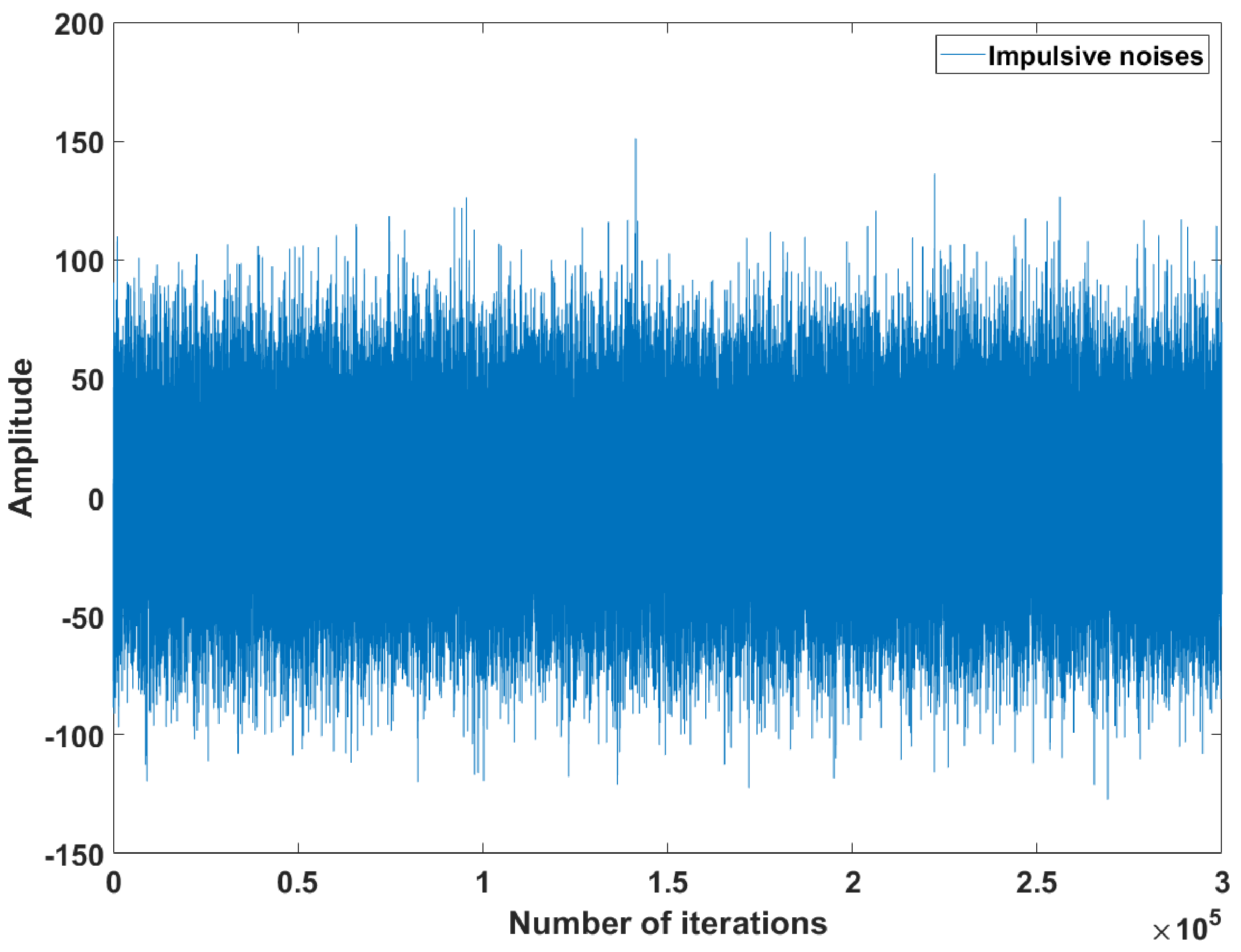
Impulsive noise v i m p ( n ) was added to the system output signal. Impulsive noise v i m p ( n ) was generated as v i m p ( n ) = k ( n ) A ( n ) , where k ( n ) is a Bernoulli process with a probability of success P [ k ( n ) = 1 ] = P r , and A ( n ) is zero-mean white Gaussian noise with power σ A 2 = 1000 σ y 2 . P r denotes the probability of impulsive-noise occurrence, and P r was set to be 0.3 for realizing harsh impulsive-noise scenarios as shown in Figure 2. The parameters for the step-size reset in the proposed algorithm were set as recommended by [23] as follows: V T = 3 m , V D = 0.75 V T , ξ = 25 , ϵ = 10 6 .
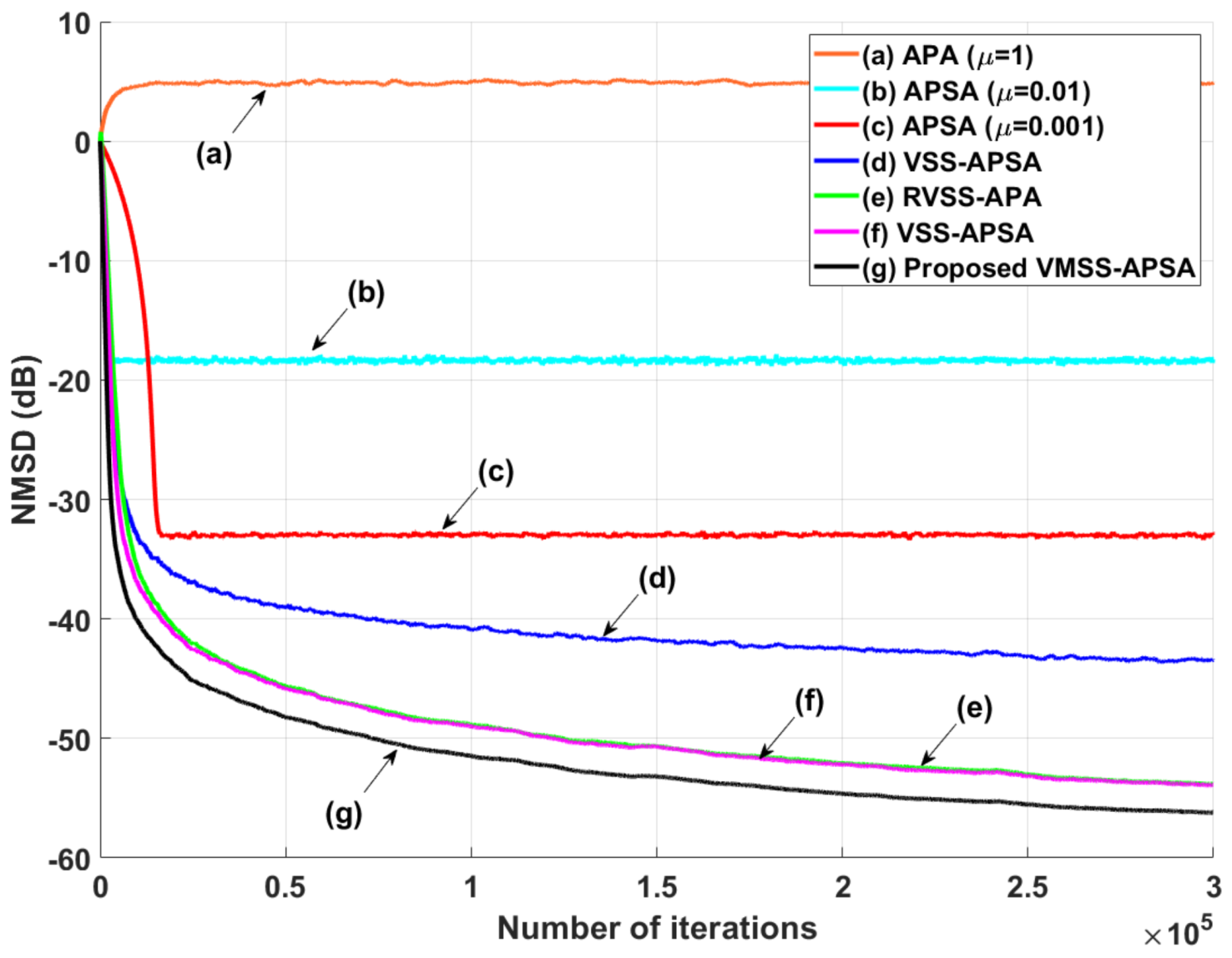
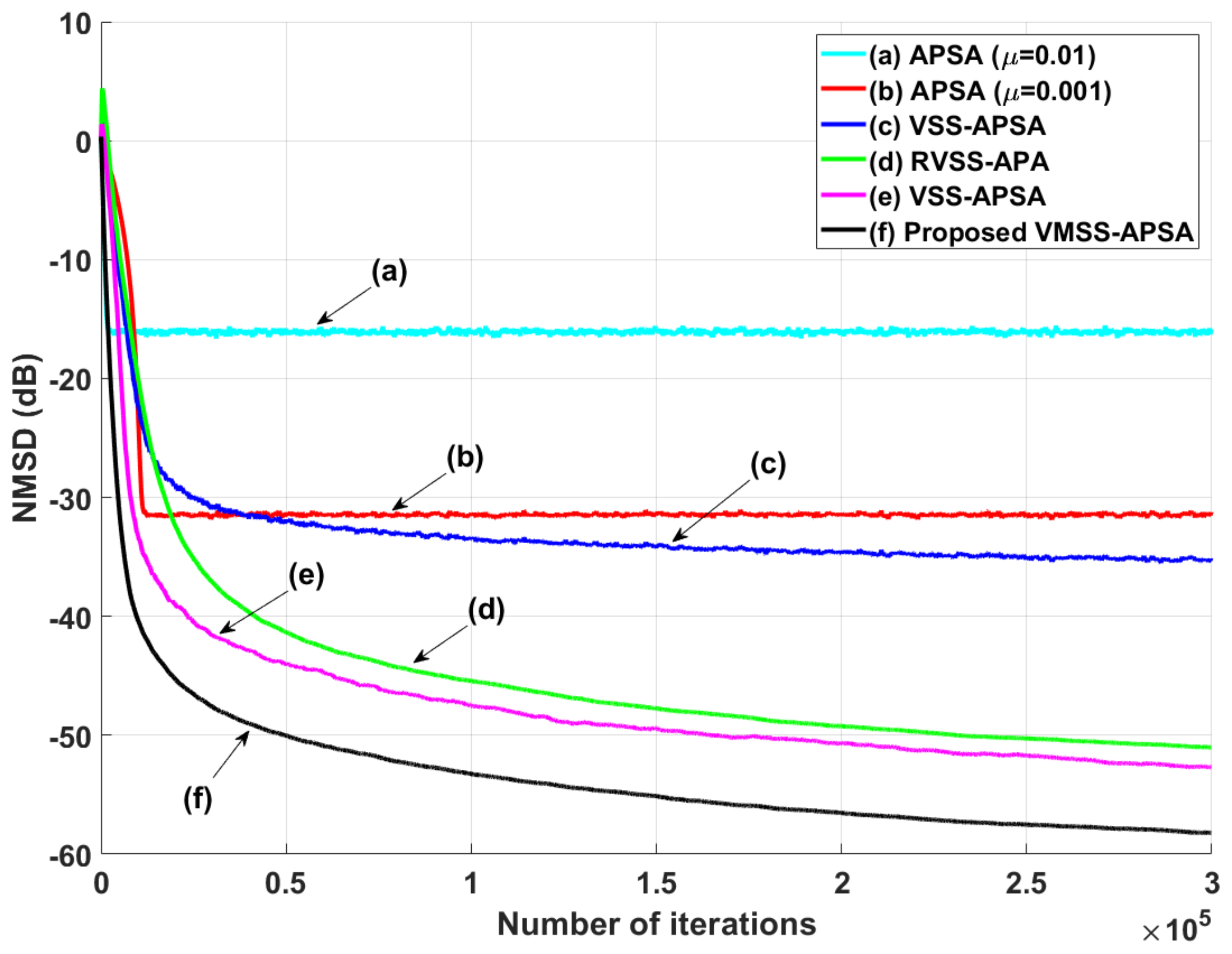
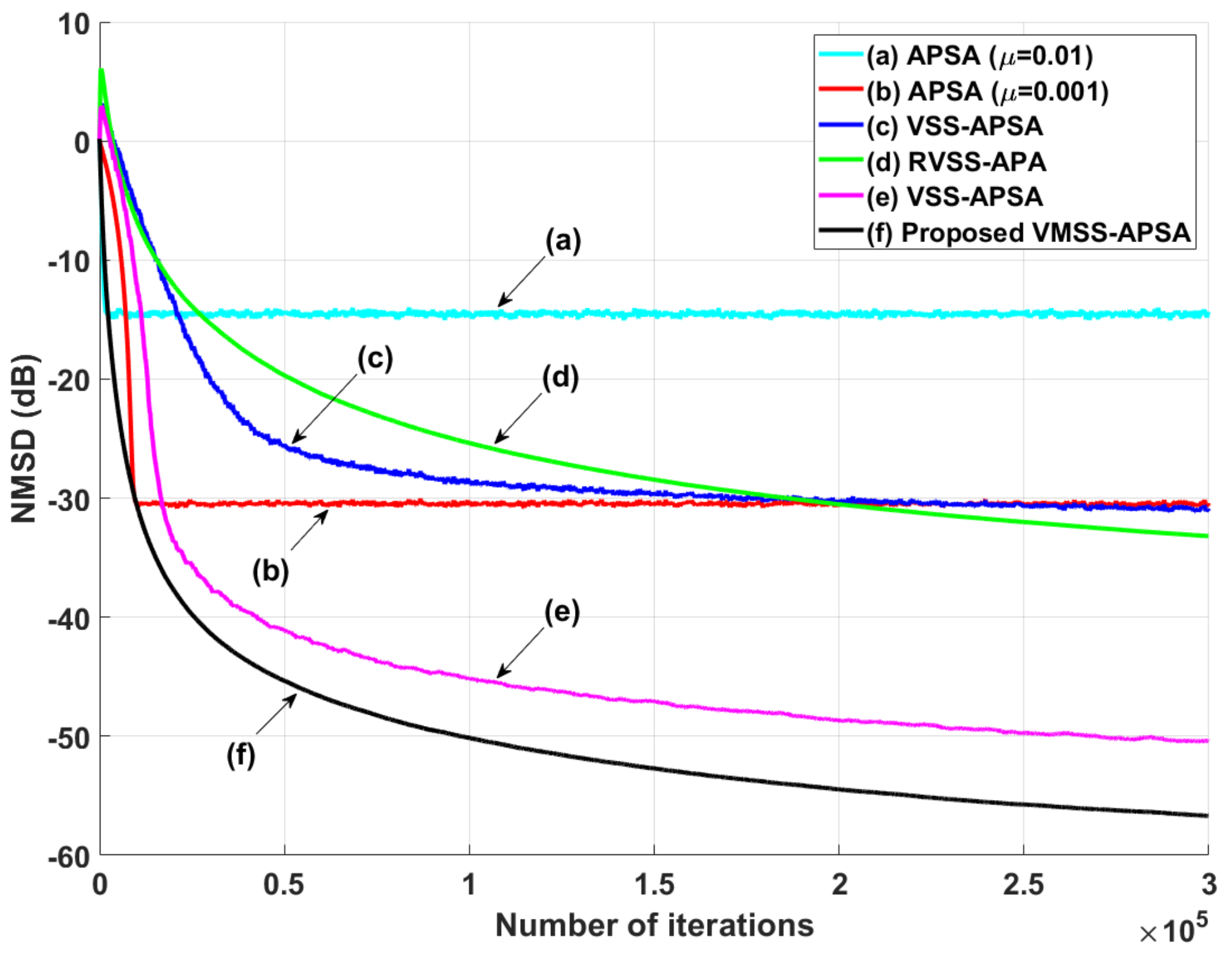
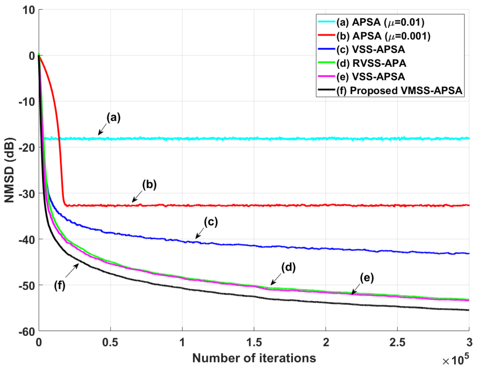
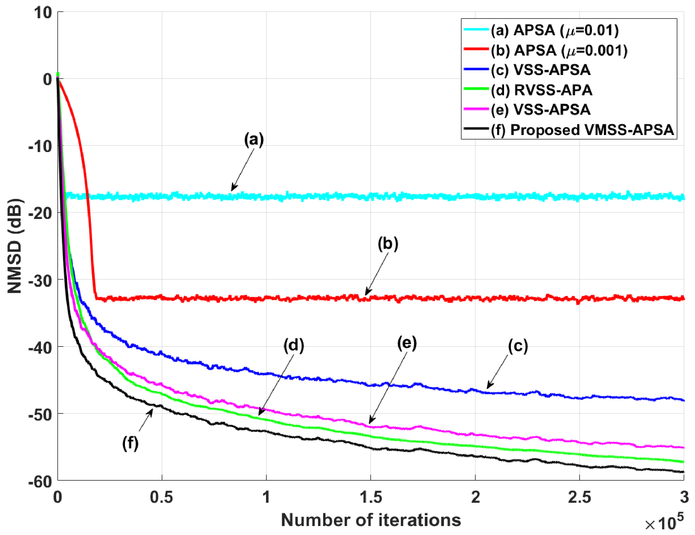
Figure 3, Figure 4 and Figure 5 show the NMSD learning curves for the original APSA, VSS-APSA, and the proposed VMSS-APSA using the white input signal with impulsive noise for various projection order levels: M = 2, 4, 6. Because impulsive noise occurred with an occurrence probability of 0.3 in the simulations, the original APA based on L 2 -norm optimization diverged, as revealed in Figure 3. Figure 6 and Figure 7 also show the NMSD learning curves for the original APSA, VSS-APSA, and the proposed VMSS-APSA using the colored input signals G 1 ( z ) and G 2 ( z ) with impulsive noise. Moreover, Figure 8 shows the NMSD learning curves for the original APSA, VSS-APSA, and the proposed VMSS-APSA using the colored input signals G 1 ( z ) with α -stable noise ( α = 1.5 ). To ensure a fair comparison between the existing VSS-APSAs and the proposed VMSS-APSA, we set the value of μ ( 0 ) and μ i ( 0 ) , 0 < i M as σ d 2 / σ u 2 m in all algorithms. As shown in Figure 3, Figure 4, Figure 5, Figure 6, Figure 7 and Figure 8, the proposed VMSS-APSA exhibited the fastest convergence rate and lowest steady-state estimation error compared with existing algorithms. In addition, the computational complexity of the proposed VMSS-APSA was moderate and similar to the existing algorithms because the additional complexity was only based on the repetitive statement in Table 1.

4.2. System Sudden-Change Scenarios

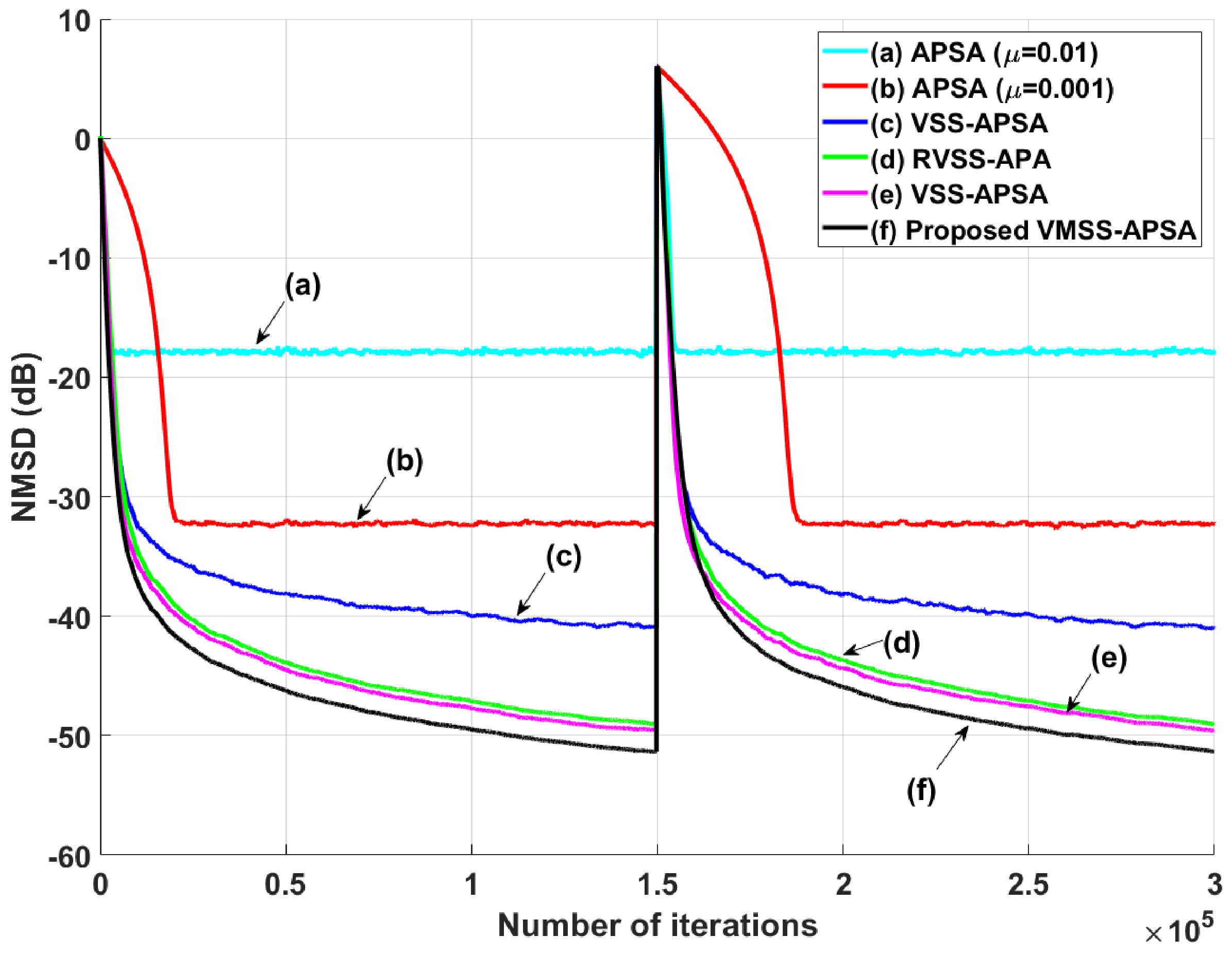
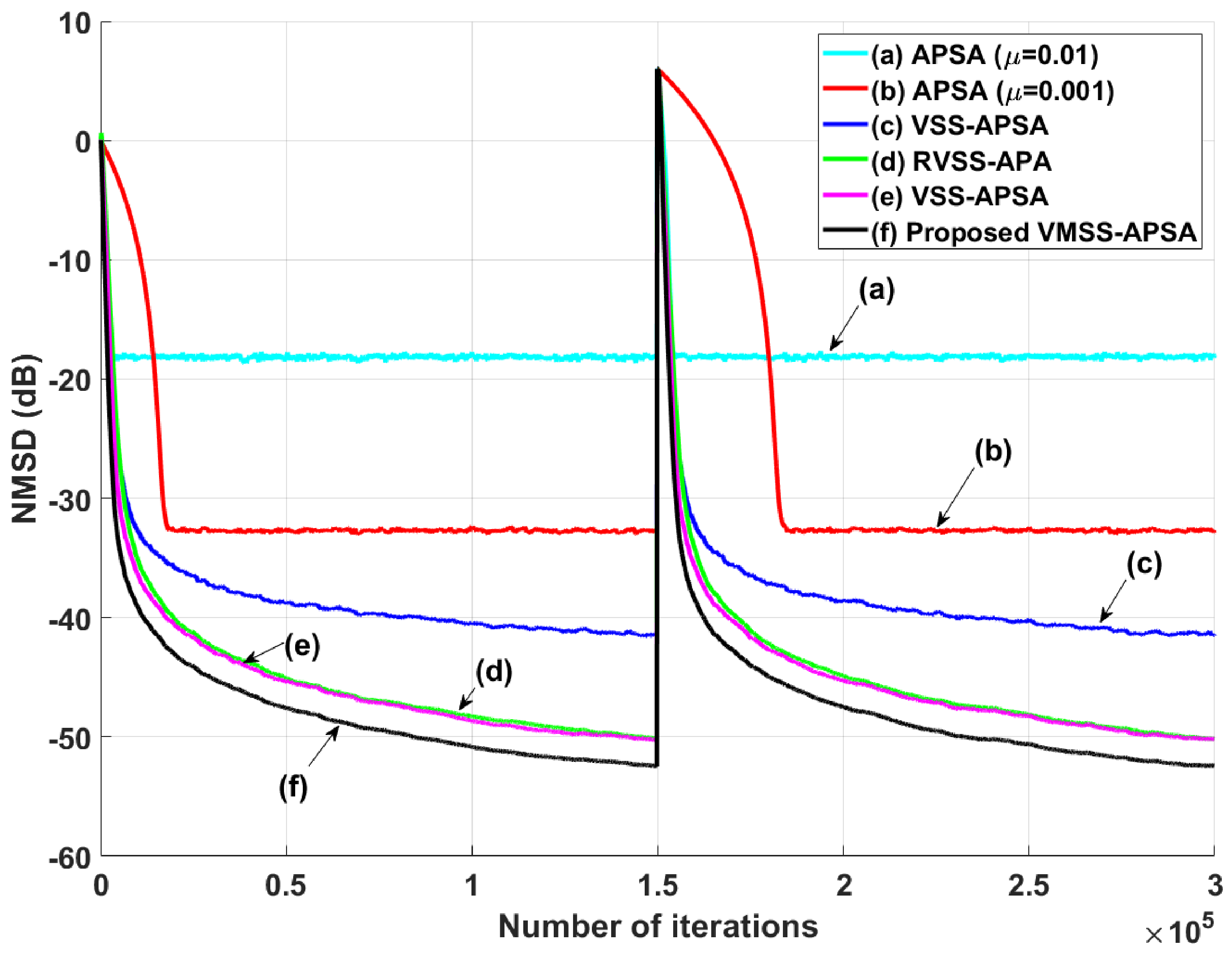
Figure 9, Figure 10 and Figure 11 show that, although the system suddenly changed, the proposed algorithm performed well because of the reset algorithm described in Section 3.3.
The parameters for the step-size reset in RVSS-APA [22] and VMSS-APSA were set consistently as recommended by [23] as follows: V T = 3 M , V D = 0.75 × V T , ξ = 25 , ϵ = 10 6 . VSMM-APSA maintained filter performance when the unknown system was suddenly changed owing to the reset algorithm after 1.5 × 10 5 iterations. Thus, from simulation results obtained under various scenarios, the performance of the proposed algorithm was verified.

5. Conclusions

This paper presented a novel variable matrix-type step-size algorithm for APSA based on the minimization of MSD. The proposed VMSS-APSA uses the upper bound of the MSD, which can be calculated using the upper bound of the L 1 -norm of the measurement noise because the MSD of APSA cannot be computed accurately. The optimal matrix-type step size can be given by minimizing the upper bound of the MSD at every iteration, and it improves the filter performance in terms of the convergence rate and steady-state estimation error. The experimental results demonstrate that the proposed VMSS-APSA has a faster convergence rate and a smaller steady-state estimation error compared with those of existing adaptive-filtering algorithms in a system-identification scenario with impulsive noise.

Author Contributions

Conceptualization and formal analysis, J.S.; investigation and validation, B.Y.P.; methodology and software W.I.L.; software and writing, J.Y. All authors have read and agreed to the published version of the manuscript.

Funding

This research received no external funding.

Institutional Review Board Statement

Not applicable.

Informed Consent Statement

Not applicable.

Data Availability Statement

Not applicable.

Acknowledgments

This research was supported by the Ministry of Trade, Industry and Energy (MOTIE), Korea through the Autonomous driving Development Innovation Program (20014476, Development of Mixed Reality-based Autonomous Driving Parts and System Evaluation Technology).

Conflicts of Interest

The authors declare no conflict of interest.

References

  1. Xiang, M.; Xia, Y.; Mandic, D.P. Performance Analysis of Deficient Length Quaternion Least Mean Square Adaptive Filters. IEEE Trans. Signal Process. 2019, 68, 65–80. [Google Scholar] [CrossRef]
  2. Zhang, R.; Zhao, H. A Novel Method for Online Extraction of Small-Angle Scattering Pulse Signals from Particles Based on Variable Forgetting Factor RLS Algorithm. Sensors 2021, 21, 5759. [Google Scholar] [CrossRef] [PubMed]
  3. Li, Y.; Wang, Y.; Sun, L. A Proportionate Normalized Maximum Correntropy Criterion Algorithm with Correntropy Induced Metric Constraint for Identifying Sparse Systems. Symmetry 2018, 10, 683. [Google Scholar] [CrossRef]
  4. Dogariu, L.-M.; Stanciu, C.L.; Elisei-Iliescu, C.; Paleologu, C.; Benesty, J.; Ciochina, S. Tensor-Based Adaptive Filtering Algorithms. Symmetry 2021, 13, 481. [Google Scholar] [CrossRef]
  5. Kumar, K.; Pandey, R.; Karthik, M.L.N.S.; Bhattacharjee, S.S.; George, N.V. Robust and sparsity-aware adaptive filters: A Review. Signal Process. 2021, 189, 108276. [Google Scholar] [CrossRef]
  6. Long, X.; Zhao, H.; Hou, X.; Quan, W. A variable regularization parameter widely linear complex-valued NLMS algorithm: Performance analysis and wind prediction. Signal Process. 2022, 201, 108731. [Google Scholar] [CrossRef]
  7. Yu, Y.; Huang, Z.; Zakharov, Y.; Lamare, R.C. Sparsity-Aware Robust Normalized Subband Adaptive Filtering Algorithms With Alternating Optimization of Parameters. IEEE Trans. Circuits Syst. II Express Briefs 2022, 69, 3934–3938. [Google Scholar] [CrossRef]
  8. Abadi, M.S.E.; Msgarani, H.; Khademiyan, S.M. Robust Variable Step-Size Affine Projection Sign Algorithm Against Impulsive Noises. Circuits Syst. Signal Process. 2019, 39, 1471–1488. [Google Scholar] [CrossRef]
  9. Yu, Y.; Lu, L.; Zahkhav, Y.; Lamare, R.C.; Chen, B. Robust Sparsity-Aware RLS Algorithms With Jointly-Optimized Parameters Against Impulsive Noise. IEEE Signal Process. Lett. 2022, 29, 1037–1041. [Google Scholar] [CrossRef]
  10. Huang, X.; Li, Y.; Zakharov, Y.V.; Li, Y.; Chen, B. Affine-Projection Lorentzian Algorithm for Vehicle Hands-Free Echo Cancellation. IEEE Trans. Veh. Technol. 2021, 70, 2561–2575. [Google Scholar] [CrossRef]
  11. Yi, Y.; He, H.; Lamare, R.C.; Chen, B. General Robust Subband Adaptive Filtering: Algorithms and Applications. IEEE/ACM Trans. Audio Speech Lang. Process. 2022, 30, 2128–2140. [Google Scholar]
  12. Ozeki, K.; Umeda, T. An adaptive filtering algorithm using an orthogonal projection to an affine subspace and its properties. Electron. Commun. Jpn. 1984, 67, 19–27. [Google Scholar] [CrossRef]
  13. Jiang, Z.; Li, Y.; Huang, X.; Jin, Z. A Sparsity-Aware Variable Kernel Width Proportionate Affine Projection Algorithm for Identifying Sparse Systems. Symmetry 2019, 11, 1218. [Google Scholar] [CrossRef]
  14. Li, G.; Wang, G.; Dai, Y.; Sun, Q.; Yang, X.; Zhang, H. Affine projection mixed-norm algorithms for robust filtering. Signal Process. 2021, 187, 108153. [Google Scholar] [CrossRef]
  15. Shin, J.; Kim, J.; Kim, T.K.; Yoo, J. Lp-Norm-like Affine Projection Sign Algorithm for Sparse System to Ensure Robustness against Impulsive Noise. Symmetry 2021, 13, 1916. [Google Scholar] [CrossRef]
  16. Shao, T.; Zheng, Y.R.; Benesty, J. An affine projection sign algorithm robust against impulsive interference. IEEE Signal Process. Lett. 2010, 17, 327–330. [Google Scholar] [CrossRef]
  17. Yang, Z.; Zheng, Y.R.; Grant, S.L. Proportionate affine projection sign algorithm for network echo cancellation. IEEE Trans. Audio Speech Lang. Process. 2011, 19, 2273–2284. [Google Scholar] [CrossRef]
  18. Yoo, J.; Shin, J.; Choi, H.; Park, P. Improved affine projection sign algorithm for sparse system identification. Electron. Lett. 2012, 48, 927–929. [Google Scholar] [CrossRef]
  19. Kim, J.H.; Chang, J.-H.; Nam, S.W. Affine projection sign algorithm with l1 minimization-based variable step-size. Signal Process. 2014, 105, 376–380. [Google Scholar] [CrossRef]
  20. Shin, J.; Yoo, J.; Park, P. Variable step-size affine projection sign algorithm. Electron. Lett. 2012, 48, 483–485. [Google Scholar] [CrossRef]
  21. Yoo, J.; Shin, J.; Park, P. Variable step-size affine projection sign algorithm. IEEE Trans. Circuits Syst. II Express Briefs 2014, 61, 274–278. [Google Scholar]
  22. Rey Vega, L.; Rey, H.; Benesty, J. A robust variable step-size affine projection algorithm. Signal Process. 2010, 90, 2806–2810. [Google Scholar] [CrossRef]
  23. Rey Vega, L.; Rey, H.; Benesty, J.; Tressens, S. A new robust variable step-size NLMS algorithm. IEEE Trans. Signal Process. 2008, 56, 1878–1893. [Google Scholar] [CrossRef]
  24. Yoo, J.; Shin, J.; Park, P. Variable step-size sign algorithm against impulsive noises. IET Signal Process. 2015, 9, 506–510–176. [Google Scholar] [CrossRef]
  25. Shin, J.; Yoo, J.; Park, P. Variable step-size sign subband adaptive filter. IEEE Signal Process. Lett. 2013, 20, 173–176. [Google Scholar] [CrossRef]
  26. Yoo, J.; Shin, J.; Park, P. A band-dependent variable step-size sign subband adaptive filter. Signal Process. 2014, 104, 407–411. [Google Scholar] [CrossRef]
  27. Tiglea, D.G.; Candido, R.; Silva, M.T.M. A Variable Step Size Adaptive Algorithm With Simple Parameter Selection. IEEE Signal Process. Lett. 2022, 29, 1774–1778. [Google Scholar] [CrossRef]
  28. Zou, Y.; Chan, S.; Ng, T. A recursive least m-estimate (RLM) adaptive filter for robust filtering in impulse noise. IEEE Signal Process. Lett. 2000, 7, 324–326. [Google Scholar] [CrossRef] [Green Version]
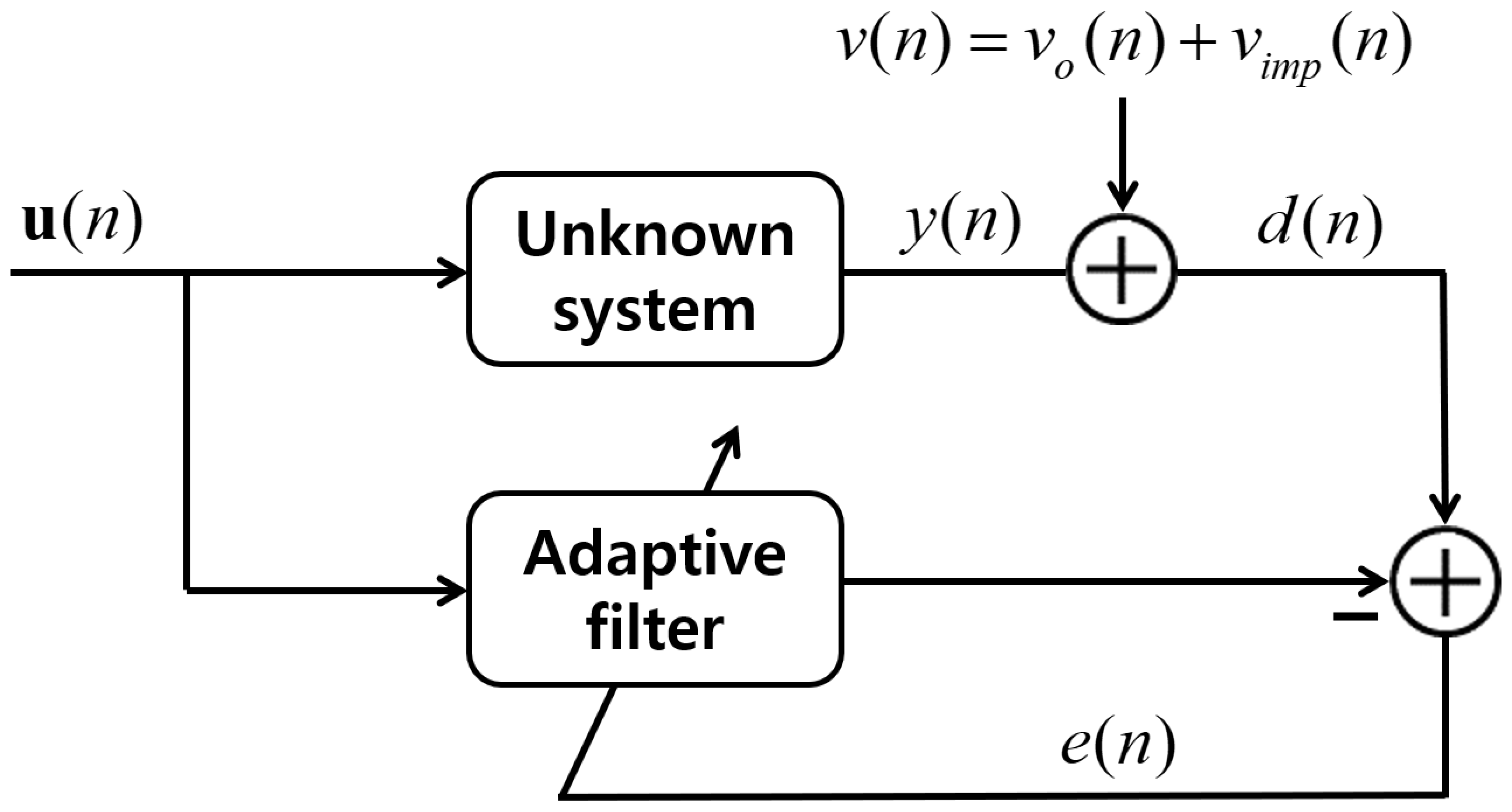
Figure 1. Structure of an adaptive filter in the presence of measurement noise v o ( n ) and impulsive noise v i m p ( n ) , with v ( n ) = v o ( n ) + v i m p ( n ) .
Symmetry 14 01985 g001
Figure 2. Characteristic of impulsive noise during 3 × 10 5 iterations (Pr = 0.3).
Symmetry 14 01985 g002
Figure 3. NMSD learning curves for the white input with impulsive noise (Pr = 0.3, M = 2), (d) VSS-APSA [20] and (f) VSS-APSA [21].
Symmetry 14 01985 g003
Figure 4. NMSD learning curves for the white input with impulsive noise (Pr = 0.3, M = 4), (d) VSS-APSA [20] and (f) VSS-APSA [21].
Symmetry 14 01985 g004
Figure 5. NMSD learning curves for the white input with impulsive noise (Pr = 0.3, M = 6), (d) VSS-APSA [20] and (f) VSS-APSA [21].
Symmetry 14 01985 g005
Figure 6. NMSD learning curves for the colored input generated by G 1 ( z ) with impulsive noise (Pr = 0.3, M = 2), (c) VSS-APSA [20] and (f) VSS-APSA [21].
Symmetry 14 01985 g006
Figure 7. NMSD learning curves for the colored input generated by G 2 (z) with impulsive noise (Pr = 0.3, M = 2), (c) VSS-APSA [20] and (f) VSS-APSA [21].
Symmetry 14 01985 g007
Figure 8. NMSD learning curves for the colored input generated by G 2 (z) with α -stable noise ( α = 1.5, M = 2), (c) VSS-APSA [20] and (f) VSS-APSA [21].
Symmetry 14 01985 g008
Figure 9. NMSD learning curves for the white input with impulsive noise (Pr = 0.3, M = 2). The system abruptly changed w o w o at iteration 1.5 × 10 5 , (c) VSS-APSA [20] and (f) VSS-APSA [21].
Symmetry 14 01985 g009
Figure 10. NMSD learning curves for the colored input generated by G 1 ( z ) with impulsive noise (Pr = 0.3, M = 2). The system abruptly changed w o w o at iteration 1.5 × 10 5 , (c) VSS-APSA [20] and (f) VSS-APSA [21].
Symmetry 14 01985 g010
Figure 11. NMSD learning curves for the colored input generated by G 2 (z) with impulsive noise (Pr = 0.3, M = 2). The system abruptly changed w o w o at iteration 1.5 × 10 5 , (c) VSS-APSA [20] and (f) VSS-APSA [21].
Symmetry 14 01985 g011
Table 1. Summary of the proposed VMSS-APSA’s pseudocode.
Initialization values: w ^ ( 0 ) = 0 , μ i ( 0 ) = σ d 2 σ u 2 m 0 < i M
Parameter setting: α = 1 M κ m
BEGIN
   FOR   i = 1 to M  DO
       β i ( n ) = | e i ( n ) | 2 π σ v sgn ( e T ( n ) ) U T ( n ) U ( n ) sgn ( e ( n ) )
      IF β i ( n ) > 0
           μ i ( n ) = α μ i ( n 1 ) + ( 1 α ) min β i ( n ) , μ i ( n 1 )
      ELSE
           μ i ( n ) = μ i ( n 1 )
      END
   ENDFOR
    w ^ ( n + 1 ) = w ^ ( n ) + U ( n ) Λ ( n ) sgn ( e ( n ) ) sgn ( e T ( n ) ) U T ( n ) U ( n ) sgn ( e ( n ) )
END
Publisher’s Note: MDPI stays neutral with regard to jurisdictional claims in published maps and institutional affiliations.