A p-Adic Matter in a Closed Universe

Abstract

In this paper, we introduce a new type of matter that has origin in p-adic strings, i.e., strings with a p-adic worldsheet. We investigate some properties of this p-adic matter, in particular its cosmological aspects. We start with crossing symmetric scattering amplitudes for p-adic open strings and related effective nonlocal and nonlinear Lagrangian which describes tachyon dynamics at the tree level. Then, we make a slight modification of this Lagrangian and obtain a new Lagrangian for non-tachyonic scalar field. Using this new Lagrangian in the weak field approximation as a matter in Einstein gravity with the cosmological constant, one obtains an exponentially expanding FLRW closed universe. At the end, we discuss the obtained results, i.e., computed mass of the scalar p-adic particle, estimated radius of related closed universe and noted p-adic matter as a possible candidate for dark matter.

1. Introduction

p-adic numbers were invented (discovered) by mathematician K. Hansel in 1897. Their initial use in physical systems modeling was conducted by I. V. Volovich [1] in 1987 by construction of some string scattering amplitudes in terms of p-adic analysis; see also [2]. This work has induced a lot of activity, not only in p-adic string theory, but also in many other sectors of modern mathematical and theoretical physics—what is now known as p-adic mathematical physics. We refer to the reviews [3,4,5,6].

Let us recall that classical theoretical physics uses mathematical methods based on real numbers, whereas quantum theory is inherently related to mathematics with complex numbers, which are algebraic extensions of real numbers. General relativity combined with quantum mechanics predicts the Planck length as the smallest length that can be measured [4]. In other words, there is breakdown of the Archimedean axiom at the Planck scale and the problem of how to use methods with real and complex numbers emerges, since their geometrical properties are based on the Archimedean norm. Then, the following question arises: are there some other numbers that could be relevant to approach the very small space–time (Planck) length? A possible answer could be related to a hypothesis [7] which assumes that space–time, at very short distances, may be non-Archimedean (ultrametric) and p-adic numbers could play some significant role. If so, then string worldsheets may be not only real but also p-adic. This was realized by the construction of some new string amplitudes replacing a real worldsheet by its analog with p-adic numbers. Strings with p-adic-valued worldsheets are called p-adic strings.

Progress in p-adic string theory has been mainly developed in two directions, namely, towards the p-adic analog of conformal field theory, in particular AdS/CFT correspondence, e.g., see [8,9]; and along an effective Lagrangian [10,11] for the scalar field, that describes all scattering amplitudes on the tree level, see [3,4] as a review for initial research. The research work contained in the present paper is based on this effective Lagrangian.

Let us mention some interesting points related to the effective Lagrangian (10) for p-adic open strings, which was constructed in 1988 [10,11]. Since it does not contain p-adic ingredients, but only real terms, there is no need to know and use p-adic analysis, which simplifies further elaboration of p-adic string theory. In fact, this Lagrangian (10) is exact at the tree level and contains a scalar field (tachyon) with a nonlocal kinetic term and nonlinear potential. It is also worth mentioning the following: demonstration of tachyon condensation [12], connection to the ordinary bosonic string in the limit $p\to 1$ [13], investigation of dynamics with infinitely many time derivatives [14] and exact solutions [15], inflation [16] and some other features (see reviews [3,5,6]).

Let us recall that p-adic strings have connections with ordinary strings not only in the limit $p\to 1$ [13,17,18] but also through an adelic product formula of ordinary and p-adic crossing symmetric Veneziano amplitudes [19,20] (see next section). Despite these connections, p-adic strings have been treated as auxiliary constructions with respect to ordinary strings, often as a toy version of the ordinary ones. However, if ordinary matter has its origin in ordinary strings, why could p-adic strings not generate p-adic matter? In this paper, we consider how non-tachyonic matter can be obtained from Lagrangian for p-adic tachyons and demonstrate that this new matter makes sense in the case of a closed universe.

This article is organized as follows: In Section 2, some basic facts about p-adic numbers, adeles, amplitudes for scattering of open p-adic strings and an effective nonlocal Lagrangian with an equation of motion are presented. Section 3 is devoted to p-adic matter; the Lagrangian for p-adic strings is slightly modified to obtain the well-defined new one, the dynamics of p-adic scalar particles is considered in weak field approximation and a cosmological solution is found and presented in the case of a closed universe fulfilled by p-adic matter with the cosmological constant. Concluding remarks, which contain some discussions on the mass of p-adic particles and the radius of the related closed universe, are the subject of Section 4. There is also an Appendix with some details on derivation of the equations of motion in the case of a nonlocal scalar field.

2. On $\mathit{p}$-Adic Strings

In this section, we recall basic facts about p-adic strings. Since they have p-adic worldsheets, we start with some mathematical background.

2.1. p-Adic Numbers, Adeles and Their Functions

For those who are not familiar with p-adic numbers, adeles and their functions, here are some basic introductory facts. To this end, it is useful to start with the field of rational numbers $\mathbb{Q}$, since $\mathbb{Q}$ is important from a physical and mathematical point of view. In physics, all numerical results of measurements are rational numbers. In mathematics, $\mathbb{Q}$ is an infinite number field. With respect to a given prime number p, any non-zero rational number x can be presented as $x=\frac{a}{b}{p}^{\nu }$, where $a,\nu \in \mathbb{Z}$ and $b\in \mathbb{N}$; further, a and b are not divisible by p. Then, by definition, the p-adic norm (also called p-adic absolute value) is ${\left|x\right|}_p=p^{-\nu }$ and ${\left|0\right|}_p=0$. One can easily show that ${\left|a\right|}_p\le 1$, for any $a\in \mathbb{Z}$ and any prime p. From the above definition, it follows the strong triangle inequality ${|x+y|}_p\le {\max \left\{\right|x|}_p{,\left|y\right|}_p\}$, i.e., the p-adic norm is an example of ultrametric (non-Archimedean) norm. The p-adic distance between $x,y\in \mathbb{Q}$ is $d_p(x,y)={|x-y|}_p$. In the same manner, as the field $\mathbb{R}$ of real numbers obtains from $\mathbb{Q}$ by completion with respect to the real distance $d(x,y)=|x-y|$, so the completion of $\mathbb{Q}$ using a p-adic distance gives the field ${\mathbb{Q}}_p$ of p-adic numbers, for any prime number p.

Any non-zero p-adic number $0\ne x\in {\mathbb{Q}}_p$ has unique representation in the following form:

$$\begin{array}{c}\hfill x=p^{\nu }\left(x_0+x_{1}p+x_2{p}^2+\dots \right),\nu \in \mathbb{Z},x_0\ne 0,x_n\in \{0,1,\dots ,p-1\},\end{array}$$

(1)

where $x_n$ are digits. For instance, $-1=p-1+(p-1)p+(p-1)p^2+\dots$ for any given prime number p.

There are mainly two kinds of functions with p-adic argument, (i) p-adic-valued functions and (ii) complex (real)-valued functions. For example, p-adic-valued elementary functions are defined by the same infinite power series as in the real case, but their convergence is subject to the p-adic distance. There are three typical complex-valued functions of the p-adic argument x:

• multiplicative character: ${\pi }_p\left(x\right)={\left|x\right|}_p^c,c\in \mathbb{C}$;
• additive character: ${\chi }_p\left(x\right)=exp\left(2\pi i{\left\{x\right\}}_p\right)$, where ${\left\{x\right\}}_p$ is a fractional part of x;
• characteristic function: ${\Omega \left(\right|x|}_p)=\left\{\begin{array}{c}{1\mathrm{if}\left|x\right|}_p\le 1,\hfill \\ {0\mathrm{if}\left|x\right|}_p>1.\hfill \end{array}\right.$

There is a well-defined integration of complex-valued functions with the Haar measure, see [4]. For example, ${\int }_{{\left|x\right|}_p\le 1}{\left|x\right|}_p^{a-1}=\frac{1-p^{-1}}{1-p^{-a}}$, where x is a p-adic variable and a is a complex number, with $\Re a>0$.

According to the Ostrowski theorem, real and p-adic numbers are all possible numbers that can be obtained by completion of $\mathbb{Q}$ with respect to any nontrivial norm on $\mathbb{Q}$. $\mathbb{Q}$ is a common subfield of $\mathbb{R}$ and all ${\mathbb{Q}}_p$.

Adeles are a concept that takes together real and p-adic numbers. By definition, an adele is the following infinite sequence:

$$\begin{array}{c}\hfill \alpha =({\alpha }_{\infty },{\alpha }_2,{\alpha }_3,\dots ,{\alpha }_p,\dots ),\end{array}$$

(2)

where ${\alpha }_{\infty }\in {\mathbb{Q}}_{\infty }\equiv \mathbb{R}$ and, for all but a finite set $\mathcal{P}$ of primes p, it must be satisfied that $x_p\in {\mathbb{Z}}_p\equiv \{x\in {\mathbb{Q}}_p{:\left|x\right|}_p\le 1\}$. ${\mathbb{Z}}_p$ is called a ring of p-adic integers. The set $A_{\mathbb{Q}}$ of all adeles over $\mathbb{Q}$ can be defined as

$$\begin{array}{c}\hfill A_{\mathbb{Q}}=\bigcup _{\mathcal{P}}\mathcal{A}\left(\mathcal{P}\right),\mathcal{A}\left(\mathcal{P}\right)=\mathbb{R}\times \prod _{p\in \mathcal{P}}{\mathbb{Q}}_p\times \prod _{p\notin \mathcal{P}}{\mathbb{Z}}_p.\end{array}$$

(3)

$A_{\mathbb{Q}}$ is called an adele ring, since it satisfies, component-wise, addition and multiplication. Note that the components of an adele can be rational numbers; thus, $\mathbb{Q}$ is naturally embedded in $A_{\mathbb{Q}}$. Hence, adeles can be viewed as a generalization of rational numbers that takes simultaneously into consideration all their completions.

There are many useful adelic product formulas which connect real and all p-adic constructions of the same form; e.g., see [4]. Some simple cases are:

• ${\pi }_{\infty }\left(x\right){\prod }_p{\pi }_p\left(x\right)=\left|x\right|{\prod }_p{\left|x\right|}_p=1$, $0\ne x\in \mathbb{Q}$;
• ${\chi }_{\infty }\left(x\right){\prod }_p{\chi }_p\left(x\right)=e^{-2\pi ix}{\prod }_p{e}^{2\pi i{\left\{x\right\}}_p}=1$, $x\in \mathbb{Q}$.

In the next subsection, we present adelic product formulas for string amplitudes.

Above, some very basic properties of p-adic numbers and adeles are presented. For more information, we refer to books [4,21,22].

2.2. p-Adic Open String Amplitudes

It is worth noticing that string theory started with the Veneziano amplitude. Let us recall that, by definition, the crossing symmetric Veneziano amplitude for the scattering of ordinary two-open strings is

$$\begin{array}{cc}\hfill A_{\infty }(a,b)& =g_{\infty }^2{\int }_{\mathbb{R}}{\left|x\right|}_{\infty }^{a-1}{|1-x|}_{\infty }^{b-1}{d}_{\infty }x\hfill \end{array}$$

(4)

$$\begin{array}{cc}\hfill & =g_{\infty }^2\frac{\zeta (1-a)}{\zeta \left(a\right)}\frac{\zeta (1-b)}{\zeta \left(b\right)}\frac{\zeta (1-c)}{\zeta \left(c\right)},a+b+c=1,\hfill \end{array}$$

(5)

where $a,b,c\in \mathbb{C}$ are related to kinematical quantities with a condition, ${|·|}_{\infty }$ denotes the usual absolute value and $\zeta$ is the Riemann zeta function. Then, the analogous p-adic Veneziano amplitude is defined as follows [2]:

$$\begin{array}{cc}\hfill A_p(a,b)& =g_p^2{\int }_{{\mathbb{Q}}_p}{\left|x\right|}_p^{a-1}{|1-x|}_p^{b-1}{d}_{p}x\hfill \end{array}$$

(6)

$$\begin{array}{cc}\hfill & =g_p^2\frac{1-p^{a-1}}{1-p^{-a}}\frac{1-p^{b-1}}{1-p^{-b}}\frac{1-p^{c-1}}{1-p^{-c}},\hfill \end{array}$$

(7)

where $a, b$ and c are the same quantities as in the above real case. It is obvious that the amplitude in (7) is symmetric under any interchange among $a, b$ and c. Note that the form of Expressions (4) and (6) is the same and contains analogous ingredients. Only the integration is different—along a real axis in (4) and over ${\mathbb{Q}}_p$ in (6). Regarding the integration of the p-adic integral in (6), one can see [3,4]. Finally, one can say that the difference between p-adic and ordinary strings is in their worldsheets, i.e., p-adic and real worldsheets, respectively. Both these kinds of strings are related to tachyons [3].

Recalling the Euler expression of the Riemann $\zeta$ function and taking the product of (7) over all primes, one obtains the Freund–Witten formula [19] for the above Veneziano amplitudes.

$$\begin{array}{c}\hfill A(a,b)=A_{\infty }(a,b)\prod _p{A}_p(a,b)=g_{\infty }^2\prod _p{g}_p^2=const.\end{array}$$

(8)

Formula (8) tells us that the amplitudes of the above p-adic and ordinary strings are on equal footing, that they may be different faces of an adelic string and that complicate ordinary amplitude with the Riemann zeta function can be expressed as the infinite product of inverse p-adic amplitudes, which are elementary and simpler functions.

By a similar procedure one can define the amplitudes for p-adic closed strings and the corresponding adelic formula also exists; as a review, see [3]. However, this article is devoted only to p-adic open strings.

2.3. Effective Field Theory for p-Adic Open Strings

It is very interesting and important that there is an effective field theory model that can reproduce the p-adic string amplitudes in (7). The corresponding action [10,11] for the scalar field $\phi \left(x\right)$ in D-dimensional Minkowski space is

$$S_p={\sigma }_p\int d^{D}x\left(-\frac{1}{2}\phi p^{-\frac{1}{2m^2}\square }\phi +\frac{1}{p+1}{\phi }^{p+1}\right),$$

(9)

where ${\sigma }_p=\frac{m^D}{g_p^2}\frac{p^2}{p-1}$, p is a prime number and $\square =-\frac{{\partial }^2}{\partial t^2}+{\sum }_{i=1}^{D-1}\frac{{\partial }^2}{\partial {x^i}^2}$ is the d’Alembert operator ($c=1$) in D-dimensional space–time. Note that Action (9) is invariant (symmetric) under discrete transformation $\phi \to -\phi$ if the prime number $p\ge 3$ and is asymmetric when $p=2.$ Field $\phi$ and mass parameter m can also depend on the prime p, but, for simplicity, we omit index p. A similar, effective field theory was also constructed for closed p-adic strings. This model (9) describes not only four-point scattering amplitudes (7) but also all higher (Koba–Nielsen) ones at the tree-level.

The corresponding Lagrangian

$${\mathcal{L}}_p={\sigma }_p\left(-\frac{1}{2}\phi p^{-\frac{1}{2m^2}\square }\phi +\frac{1}{p+1}{\phi }^{p+1}\right),$$

(10)

contains a nonlocal kinetic term with infinitely many space–time derivatives in the form $p^{-\frac{1}{2m^2}\square }$ and nonlinear potential with ${\phi }^{p+1}$ interaction.

The equation of motion (EoM) related to Lagrangian (10) is

$$\begin{array}{c}\hfill p^{-\frac{1}{2m^2}\square }\phi \equiv e^{-\frac{lnp}{2m^2}\square }\phi ={\phi }^p.\end{array}$$

(11)

There are trivial solutions $\phi =0,+1$ for any p as well as $\phi =-1$, when $p\ne 2$. In the Minkowski space, there is a nontrivial homogeneous and isotropic time-dependent solution

$$\begin{array}{c}\hfill \phi \left(t\right)=p^{\frac{1}{2(p-1)}}exp\left(\frac{p-1}{2plnp}{m}^2{t}^2\right)\end{array}$$

(12)

and also an inhomogeneous solution in any spatial direction $x^i$

$$\begin{array}{c}\hfill \phi \left(x^i\right)=p^{\frac{1}{2(p-1)}}exp\left(-\frac{p-1}{2plnp}{m}^2{\left(x^i\right)}^2\right).\end{array}$$

(13)

In D-dimensional space–time, the solution is [15]

$$\begin{array}{c}\hfill \phi \left(x\right)=p^{\frac{D}{2(p-1)}}exp\left(-\frac{p-1}{2plnp}{m}^2{x}^2\right),x^2=-t^2+\sum _{i=1}^{D-1}{\left(x^i\right)}^2.\end{array}$$

(14)

For example, the solution in (12) can be obtained employing the identity

$$\begin{array}{c}\hfill e^{A{\partial }_t^2}{e}^{B{t}^2}=\frac{1}{\sqrt{1-4AB}}{e}^{\frac{B{t}^2}{1-4AB}},1-4AB>0.\end{array}$$

(15)

All the above solutions of EoM (11) are unstable [23].

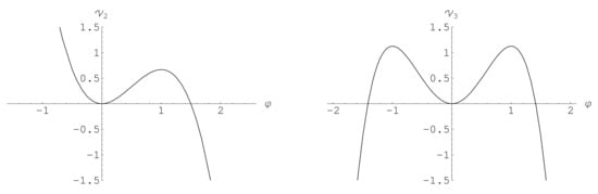
The corresponding potential ${𝒱}_p\left(\phi \right)=-{\mathcal{L}}_p(\square =0)$ of Lagrangian (10) is

$$\begin{array}{c}\hfill {𝒱}_p\left(\phi \right)={\sigma }_p\left[\frac{1}{2}{\phi }^2-\frac{1}{p+1}{\phi }^{p+1}\right],\end{array}$$

(16)

which has local minimum ${𝒱}_p\left(0\right)=0$ for all p and local maxima ${𝒱}_2\left(1\right)=\frac{{\sigma }_2}{6}$ and ${𝒱}_p(\pm 1)={\sigma }_p\frac{p-1}{2(p+1)}$, when $p\ne 2$. When $p=2$ and $p=3$, these potentials are illustrated at Figure 1. When $p\ne 2$, all potentials are an even (symmetric) function of $\phi$.

Figure 1. The 2-adic string potential ${𝒱}_2\left(\phi \right)$ (on the left) and 3-adic potential ${𝒱}_3\left(\phi \right)$ (on the right) of standard Lagrangian (10), where potential is presented by Expression (16) with ${\sigma }_p=1$.

Let us consider the above scalar field $\phi$ in a vicinity of its unstable value $\phi =1$, i.e., let us take $\phi =1+\eta$, where $\left|\eta \right|\ll 1$. Then, EoM (11) becomes

$$\begin{array}{c}\hfill p^{-\frac{1}{2m^2}\square }(1+\eta )={(1+\eta )}^p\approx (1+p\eta ),⟹p^{-\left(\frac{M^2}{2m^2}+1\right)}\eta =\eta ,\end{array}$$

(17)

which gives $M^2=-2m^2$, i.e., the scalar field $\eta \left(\phi \right)$ presents a tachyon.

3. Scalar $\mathit{p}$-Adic Matter

We are now going to slightly modify Lagrangian (10) with the intention to obtain a new Lagrangian for a similar scalar particle which is not a tachyon. Another direction of research based on Lagrangian (10) is towards zeta strings that take into account the effects of p-adic strings over all primes p; see [24] and references therein.

3.1. Non-Tachyonic p-Adic Scalar Field in Minkowski Space

To this end, for some prime p, let us consider the transition $-m^2\to m^2$ in (10); see an initial consideration in [25,26]. To differ from a tachyon, we denote this new scalar p-adic field by $\varphi .$ Note that, by replacing $-m^2$ with $m^2$, the new related Lagrangian becomes

$$\begin{array}{c}\hfill L_p\left(\varphi \right)={(-1)}^{\frac{D}{2}}{\sigma }_p\left[-\frac{1}{2}\varphi p^{\frac{\square }{2m^2}}\varphi +\frac{1}{p+1}{\varphi }^{p+1}\right],\end{array}$$

(18)

where the change ${\sigma }_p\to {(-1)}^{\frac{D}{2}}{\sigma }_p$ is taken into account. Depending on space–time dimensionality D, we have

$$\begin{array}{c}\hfill {(-1)}^{\frac{D}{2}}=\left\{\begin{array}{c}+1\mathrm{if}D=4k\hfill \\ -1\mathrm{if}D=4k+2\hfill \\ +i\mathrm{if}D=4k+1\hfill \\ -i\mathrm{if}D=4k+3,\hfill \end{array}\right.\end{array}$$

(19)

where $k\in \mathbb{N}$. According to (19), it follows that Lagrangian (18) can be real only when space–time dimensionality $D=2,4,6,\dots$ Note that the kinetic term is positive when $D=4k+2$, i.e., including $D=10$ and 26, which are critical dimensions in string theory.

The equation of motion for the scalar field $\varphi$ is

$$\begin{array}{c}\hfill p^{\frac{\square }{2m^2}}\varphi ={\varphi }^p\end{array}$$

(20)

and it has the same trivial solutions as the previous field $\phi$, i.e., $\varphi =0$ and $\varphi =1$ for any p and $\varphi =-1$, if $p\ne 2$. There are also nontrivial solutions, such as (12)–(14), where one has to replace $m^2$ with $-m^2$.

When $D=2+4k$, Lagrangian (18) is

$$\begin{array}{c}\hfill L_p\left(\varphi \right)={\sigma }_p\left[\frac{1}{2}\varphi p^{\frac{\square }{2m^2}}\varphi -\frac{1}{p+1}{\varphi }^{p+1}\right],\end{array}$$

(21)

and the corresponding potential becomes

$$\begin{array}{c}\hfill V_p\left(\varphi \right)={\sigma }_p\left[\frac{1}{p+1}{\varphi }^{p+1}-\frac{1}{2}{\varphi }^2\right].\end{array}$$

(22)

Note that, now, $L_p\left(\varphi \right)=-{\mathcal{L}}_p\left(\phi \right)$ and $V_p\left(\varphi \right)=-{𝒱}_p\left(\phi \right)$.

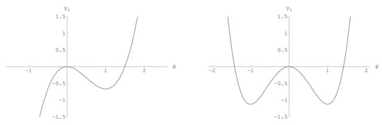
The trivial solutions of EoM (20) have the following meaning: ${\varphi }_p=0$ is a local maximum and ${\varphi }_2=+1$ and ${\varphi }_p=\pm 1$, with $p\ne 2$, are local minima; see also Figure 2.

Figure 2. New potentials $V_2\left(\varphi \right)$ and $V_3\left(\varphi \right)$, which are defined by (22). This is the same potential as in Figure 1, but with opposite sign.

Let us consider field $\varphi$ around minima $\varphi =\pm 1$. For example, let $\varphi =1+\theta$ in the case when $D=2+4k$. Then, the EoM for weak field $\theta$, i.e., $\left|\theta \right|\ll 1$, becomes

$$\begin{array}{c}\hfill p^{\frac{\square }{2m^2}}(1+\theta )={(1+\theta )}^p,\Rightarrow p^{\frac{\square }{2m^2}}\theta =p\theta .\end{array}$$

(23)

Let us look for a solution of EoM $p^{\frac{\square }{2m^2}}\theta =p\theta$ in some detail. In fact, we have equation

$$\begin{array}{c}\hfill e^{\frac{lnp}{2m^2}\square }\theta =\left(1+\frac{lnp}{2m^2}\square +{\left(\frac{lnp}{2m^2}\right)}^2\frac{{\square }^2}{2!}+\dots \right)\theta =p\theta ,\end{array}$$

(24)

which has a solution when the following Klein–Gordon equation is satisfied:

$$\begin{array}{c}\hfill (\square -2m^2)\theta =0,\mathrm{where}\square =-\frac{{\partial }^2}{\partial t^2}+\sum _{i=1}^{D-1}\frac{{\partial }^2}{\partial {x^i}^2}\end{array}$$

(25)

and we have that $\theta \sim e^{\pm i(-Et+\overrightarrow{k}\overrightarrow{x})}$ is a scalar field with $E^2=2m^2+{\overrightarrow{k}}^2$.

The above consideration is related to a scalar field in the D-dimensional Minkowski space. In the next subsection, we want to study some cosmological aspects of field $\theta$ in 4-dimensional space–time.

3.2. A Closed Universe with p-Adic Matter

Let us start with a 4-dimensional gravity with a nonlocal scalar field $\varphi$ and cosmological constant $\Lambda$, given by the Einstein–Hilbert action

$$S=\gamma \int \sqrt{-g}{d}^{4}x(R-2\Lambda )+S_m,$$

(26)

where $\gamma =\frac{1}{16\pi G}$, R is the Ricci scalar and

$$S_m=\sigma \int \sqrt{-g}{d}^{4}x\left(\frac{1}{2}\varphi F(\square )\varphi -U\left(\varphi \right)\right),$$

(27)

where $F(\square )={\sum }_{n=0}^{\infty }{f}_n{\square }^n$ is a nonlocal operator and $U\left(\varphi \right)$ is a part of the potential. Note that, now, $\square ={\nabla }_{\mu }{\nabla }^{\mu }=\frac{1}{\sqrt{-g}}{\partial }_{\mu }\sqrt{-g}{g}^{\mu \nu }{\partial }_{\nu }$.

According to the variation in Action (26), with respect to $\delta g^{\mu \nu }$ and $\delta \varphi$ and the principle of least action, the equations of motion for gravity field $g_{\mu \nu }$ and scalar field $\varphi$ are as follows:

$$\begin{array}{cc}\hfill & \gamma (G_{\mu \nu }+\Lambda g_{\mu \nu })-\frac{\sigma }{4}{g}_{\mu \nu }\varphi F(\square )\varphi +g_{\mu \nu }\frac{\sigma }{2}U\left(\varphi \right)+\frac{\sigma }{4}{\Omega }_{\mu \nu }\left(\varphi \right)=0,\hfill \end{array}$$

(28)

$$\begin{array}{cc}\hfill & F(\square )\varphi -U^{\prime }\left(\varphi \right)=0,\hfill \end{array}$$

(29)

where

$$\begin{array}{cc}\hfill {\Omega }_{\mu \nu }\left(\varphi \right)=& \sum _{n=1}^{\infty }{f}_n\sum _{\ell =0}^{n-1}[g_{\mu \nu }\left({\nabla }^{\alpha }{\square }^{\ell }\varphi {\nabla }_{\alpha }{\square }^{n-1-\ell }\varphi +{\square }^{\ell }\varphi {\square }^{n-\ell }\varphi \right)\hfill \\ \hfill & -2{\nabla }_{\mu }{\square }^{\ell }\varphi {\nabla }_{\nu }{\square }^{n-1-\ell }\varphi ].\hfill \end{array}$$

(30)

For details about the derivation of Equations of motion (28), we refer to [27]; see also Appendix A.

As a matter of interest, we take the p-adic scalar field given by its Action (21)

$$S_p={\sigma }_p\int \sqrt{-g}{d}^{4}x\left(\frac{1}{2}\varphi p^{\frac{1}{2m^2}\square }\varphi -\frac{1}{p+1}{\varphi }^{p+1}\right),$$

(31)

where, again, ${\sigma }_p=\frac{m_p^D}{g_p^2}\frac{p^2}{p-1}$ and p is a prime number. Note that, in (31), we have 4-dimensional space–time, but this takes the same signs in the Lagrangian as in the case $D=4k+2$. The reason for this choice is to have the correct sign in front of the kinematic term.

The equation of motion for p-adic field $\varphi$ has the same form as the previous one, (20), i.e.,

$$\begin{array}{c}\hfill p^{\frac{1}{2m^2}\square }\varphi \equiv e^{\frac{lnp}{2m^2}\square }\varphi ={\varphi }^p,\end{array}$$

(32)

but □ now depends on the gravity field $g_{\mu \nu }$. It has the same trivial solutions, as in the Minkowski space–time.

The potential $V_p\left(\varphi \right)$ is already given by Expression (22) and $V_2$ and $V_3$ are presented in Figure 2.

In the sequel, we are interested in cosmological solutions of the Equations of motion (28) and (29) in the homogeneous and isotropic space given by the Friedmann–Lemaître–Robertson–Walker (FLRW) metric, as follows:

$$\begin{array}{c}\hfill d{s}^2=-d{t}^2+a^2\left(t\right)\left(\frac{d{r}^2}{1-k{r}^2}+r^{2}d{\theta }^2+r^2{sin}^2\theta d{\phi }^2\right),\end{array}$$

(33)

where $a\left(t\right)$ is the cosmic scale factor and $k=0,+1,-1$ for the plane, closed and open universe, respectively. Owing to the symmetries of the FLRW metric, there are only two independent Equations of motion (28), which are usually trace

$$\begin{array}{c}\hfill 4\Lambda -R-\sigma \varphi F(\square )\varphi +2\sigma U\left(\varphi \right)+\frac{\sigma }{4}\Omega =0\end{array}$$

(34)

and 00-component

$$\begin{array}{c}\hfill \gamma (G_{00}-\Lambda )+\frac{\sigma }{4}\varphi F(\square )\varphi -\frac{\sigma }{2}U\left(\varphi \right)+\frac{\sigma }{4}{\Omega }_{00}\left(\varphi \right)=0,\end{array}$$

(35)

where $\Omega =g^{\mu \nu }{\Omega }_{\mu \nu }$. We return to (34) and (35) after some elaboration of the EoM for field $\varphi$ in (32).

Let us look for a solution of (32) in a weak field approximation around local minimum $\varphi =1$, that is, $\varphi =1+\theta$, where $\left|\theta \right|\ll 1$. As in (23), again, we have

$$\begin{array}{c}\hfill p^{\frac{\square }{2m^2}}(1+\theta )={(1+\theta )}^p,\Rightarrow p^{\frac{\square }{2m^2}}\theta =p\theta ,\end{array}$$

(36)

where, now,

$$\begin{array}{c}\hfill \square =-\frac{{\partial }^2}{\partial t^2}-3H\frac{\partial }{\partial t},H=\frac{\dot{a}}{a}\end{array}$$

(37)

and H is the Hubble parameter.

Equation

$$\begin{array}{c}\hfill p^{\frac{\square }{2m^2}}\theta =p\theta \end{array}$$

(38)

has solution if there is a solution of $\square \theta =2m^2\theta$, i.e.,

$$\begin{array}{c}\hfill \frac{{\partial }^2\theta }{\partial t^2}+3H\frac{\partial \theta }{\partial t}+2m^2\theta =0,\end{array}$$

(39)

where the Hubble parameter $H=\dot{a}/a$ may be a function of cosmic time, which depends on the scale factor $a\left(t\right)$. The simplest case is $H=constant$ and it corresponds to the scale factor $a\left(t\right)=A{e}^{Ht}$. When H is constant, Equation (39) is a linear differential equation with constant coefficients and has solution in the form $\theta \left(t\right)=C{e}^{\lambda t}$, where $\lambda$ must satisfy the quadratic equation

$$\begin{array}{c}\hfill {\lambda }^2+3H\lambda +2m^2=0.\end{array}$$

(40)

The solution of Equation (40) has the form ${\lambda }_{1,2}=\frac{-3H\pm \sqrt{9H^2-8m^2}}{2}$, where H and m can be connected as $H=\pm m$, which yields the simple solutions ${\lambda }_{+,-}=\pm m.$ It follows that the general solution of Equation (39) can be written in the form

$$\begin{array}{c}\hfill \theta \left(t\right)=C_{-}{e}^{-mt}+C_{+}{e}^{+mt}={\theta }_{-}\left(t\right)+{\theta }_{+}\left(t\right),\end{array}$$

(41)

where $C_{-}$ and $C_{+}$ are integration constants. Note that H and $\lambda$ must have opposite sign. Hence, we have the following pairs:

$$\begin{array}{cc}\hfill & \left(a_{+}\left(t\right),{\theta }_{-}\left(t\right)\right):a_{+}\left(t\right)=A_{+}{e}^{+mt},{\theta }_{-}\left(t\right)=C_{-}{e}^{-mt},\hfill \end{array}$$

(42)

$$\begin{array}{cc}\hfill & \left(a_{-}\left(t\right),{\theta }_{+}\left(t\right)\right):a_{-}\left(t\right)=A_{-}{e}^{-mt},{\theta }_{+}\left(t\right)=C_{+}{e}^{+mt},.\hfill \end{array}$$

(43)

The next step is to explore how the solution in (41) satisfies the corresponding equations of motion for a gravitational field. To this end, we have to rewrite the Einstein–Hilbert action with weak field approximation for scalar field $\varphi$, i.e., we have to rewrite (26) in terms of field $\theta$. The corresponding action is

$$\begin{array}{c}\hfill S=\gamma \int d^{4}x\sqrt{-g}(R-2\Lambda )+{\sigma }_p\int d^{4}x\sqrt{-g}\left(\frac{1}{2}\theta p^{\frac{\square }{2m^2}}\theta -\frac{p}{2}{\theta }^2+{\alpha }_p\right),\end{array}$$

(44)

where ${\alpha }_p=\frac{p-1}{2(p+1)}$.

The potential $V_p\left(\theta \right)=-L_p(\square =0)$ is

$$\begin{array}{c}\hfill V_p\left(\theta \right)={\sigma }_p\left(\frac{p-1}{2}{\theta }^2-{\alpha }_p\right)\end{array}$$

(45)

and it has the form resembling that of the harmonic oscillator.

We can now return to the Equations of motion (34) and (35). With the relevant replacements

$$\begin{array}{c}\hfill \varphi \to \theta ,\sigma \to {\sigma }_p,U\left(\theta \right)=\frac{p}{2}{\theta }^2-{\alpha }_p,\end{array}$$

(46)

we have

$$\begin{array}{cc}\hfill & \gamma (4\Lambda -R)-{\sigma }_p\theta F(\square )\theta +2{\sigma }_p(\frac{p}{2}{\theta }^2-{\alpha }_p)+\frac{{\sigma }_p}{4}\Omega =0,\hfill \end{array}$$

(47)

$$\begin{array}{cc}\hfill & \gamma (G_{00}-\Lambda )+\frac{{\sigma }_p}{4}\theta F(\square )\theta -\frac{{\sigma }_p}{2}(\frac{p}{2}{\theta }^2-{\alpha }_p)+\frac{{\sigma }_p}{4}{\Omega }_{00}\left(\theta \right)=0,\hfill \end{array}$$

(48)

where

$$\begin{array}{c}\hfill F(\square )=p^{\frac{\square }{2m^2}}=\sum _{n=0}^{\infty }{\left(\frac{lnp}{2m^2}\right)}^n\frac{1}{n!}{\square }^n=\sum _{n=0}^{\infty }{f}_n{\square }^n.\end{array}$$

(49)

We show above that there is a field $\theta$ which satisfies the EoM $p^{\frac{\square }{2m^2}}\theta =p\theta .$ This simplifies the above equations and we come to

$$\begin{array}{cc}\hfill & \gamma (4\Lambda -R)-2{\sigma }_p{\alpha }_p+\frac{{\sigma }_p}{4}\Omega \left(\theta \right)=0,\hfill \end{array}$$

(50)

$$\begin{array}{cc}\hfill & \gamma (G_{00}-\Lambda )+\frac{{\sigma }_p}{2}{\alpha }_p+\frac{{\sigma }_p}{4}{\Omega }_{00}\left(\theta \right)=0.\hfill \end{array}$$

(51)

Let us recall that, in the FLRW metric,

$$\begin{array}{c}\hfill G_{00}=3\left(\frac{{\dot{a}}^2}{a^2}+\frac{k}{a^2}\right),R=6\left(\frac{\ddot{a}}{a}+\frac{{\dot{a}}^2}{a^2}+\frac{k}{a^2}\right).\end{array}$$

(52)

Computation (52) for the scale factors $a_{+}\left(t\right)=A_{+}{e}^{+mt}$ and $a_{-}\left(t\right)=A_{-}{e}^{-mt}$ gives

$$\begin{array}{cc}\hfill & G_{00}^{(+)}=3\left(m^2+\frac{k}{a_{+}^2}\right)=3\left(m^2+\frac{k}{A_{+}^2}{e}^{-2mt}\right),\hfill \end{array}$$

(53)

$$\begin{array}{cc}\hfill & G_{00}^{(-)}=3\left(m^2+\frac{k}{a_{-}^2}\right)=3\left(m^2+\frac{k}{A_{-}^2}{e}^{+2mt}\right),\hfill \end{array}$$

(54)

$$\begin{array}{cc}\hfill & R_{+}=6\left(2m^2+\frac{k}{a_{+}^2}\right)=6\left(2m^2+\frac{k}{A_{+}^2}{e}^{-2mt}\right),\hfill \end{array}$$

(55)

$$\begin{array}{cc}\hfill & R_{-}=6\left(2m^2+\frac{k}{a_{-}^2}\right)=6\left(2m^2+\frac{k}{A_{-}^2}{e}^{+2mt}\right).\hfill \end{array}$$

(56)

Direct calculation of $\Omega \left(\theta \right)=g^{\mu \nu }{\Omega }_{\mu \nu }\left(\theta \right)$ and ${\Omega }_{00}\left(\theta \right)$, where (see (31))

$$\begin{array}{cc}\hfill {\Omega }_{\mu \nu }\left(\theta \right)=& \sum _{n=1}^{\infty }{f}_n\sum _{\ell =0}^{n-1}[g_{\mu \nu }\left({\nabla }^{\alpha }{\square }^{\ell }\theta {\nabla }_{\alpha }{\square }^{n-1-\ell }\theta +{\square }^{\ell }\varphi {\square }^{n-\ell }\theta \right)\hfill \\ \hfill & -2{\nabla }_{\mu }{\square }^{\ell }\theta {\nabla }_{\nu }{\square }^{n-1-\ell }\theta ],\hfill \end{array}$$

(57)

yields

$$\begin{array}{cc}\hfill & {\Omega }_{-}=\Omega \left({\theta }_{-}\right)=3plnp{\theta }_{-}^2=3plnp{C}_{-}^2{e}^{-2mt},\hfill \end{array}$$

(58)

$$\begin{array}{cc}\hfill & {\Omega }_{+}=\Omega \left({\theta }_{+}\right)=3plnp{\theta }_{+}^2=3plnp{C}_{+}^2{e}^{+2mt},\hfill \end{array}$$

(59)

$$\begin{array}{cc}\hfill & {\Omega }_{00}^{(-)}={\Omega }_{00}\left({\theta }_{-}\right)=-\frac{3}{2}plnp{\theta }_{-}^2=-\frac{3}{2}plnp{C}_{-}^2{e}^{-2mt},\hfill \end{array}$$

(60)

$$\begin{array}{cc}\hfill & {\Omega }_{00}^{(+)}={\Omega }_{00}\left({\theta }_{+}\right)=-\frac{3}{2}plnp{\theta }_{+}^2=-\frac{3}{2}plnp{C}_{+}^2{e}^{+2mt}.\hfill \end{array}$$

(61)

One can now easily verify that EoM (50) and (51) are satisfied in the following way:

$$\begin{array}{cc}\hfill & \gamma (4\Lambda -R_{\pm })-2{\sigma }_p{\alpha }_p+\frac{{\sigma }_p}{4}{\Omega }_{\mp }=0,\hfill \end{array}$$

(62)

$$\begin{array}{cc}\hfill & \gamma (G_{00}^{(\pm )}-\Lambda )+\frac{{\sigma }_p}{2}{\alpha }_p+\frac{{\sigma }_p}{4}{\Omega }_{00}^{\mp }=0,\hfill \end{array}$$

(63)

with the conditions

$$\begin{array}{c}\hfill 6\gamma m^2+{\sigma }_p{\alpha }_p-2\gamma \Lambda =0,plnp{\sigma }_p{A}_{\pm }^2{C}_{\mp }^2-8\gamma k=0,k=+1,\end{array}$$

(64)

or, in a more explicit form,

$$\begin{array}{cc}\hfill & \Lambda =3m^2+\frac{4\pi G}{g^2}\frac{p^2}{p-1}{m}^4,\hfill \end{array}$$

(65)

$$\begin{array}{cc}\hfill & \frac{1}{{\left(A_{\pm }{C}_{\mp }\right)}^2}=\frac{2\pi G}{g^2}\frac{p^{3}lnp}{p-1}{m}^4.\hfill \end{array}$$

(66)

Therefore, there is a solution of the corresponding equations of motion only in the pair form $\left(a_{\pm }\left(t\right),{\theta }_{\mp }\left(t\right)\right).$

4. Concluding Remarks

It is worth noting that (65) contains the connection between the cosmological constant $\Lambda$ and mass m of a p-adic scalar particle (that we call p-adic scalaron or p-scalaron). For a small mass m, as well as not a big value of prime number p (it makes sense to take $p=3$) and $g^2\ge 1$, one can neglect the second term on the RHS with respect to $3m^2$. As a result, one obtains $\Lambda \approx 3m^2$, which is written in the natural units ($\hslash =c=1$). In the international system of units (SI), the previous relation should be rewritten as

$$\begin{array}{c}\hfill m\approx \frac{\hslash }{c^2}\sqrt{\frac{\Lambda }{3}}.\end{array}$$

(67)

From (67), we can compute the approximate value of mass m, where

$$\hslash =1.05\times {10}^{-34}{\mathrm{m}}^2\mathrm{kg}/\mathrm{s},c=3\times {10}^8\mathrm{m}/\mathrm{s}\mathrm{and}\Lambda =3H^2{\Omega }_{\Lambda }=9.8\times {10}^{-36}{\mathrm{s}}^{-2}.$$

We obtain that the mass of p-scalaron is

$$m\approx 2.1\times {10}^{-69}\mathrm{kg},$$

(68)

which is about a ${10}^{-39}$ part of the mass of the electron ($m_e=9.1\times {10}^{-31}\mathrm{kg}$). Note that, in the above approximation (67), the mass of the p-adic scalaron does not depend on p.

Equality (66) tells us that the product of the radius $R=A_{\pm }$ of the closed universe under consideration and amplitude $C_{\mp }$ of the p-adic scalaron field is a constant that depends on the p-scalaron’s mass m. Rewriting (66) and using the SI system, we have

$$A_{+}=P_p\sqrt{\frac{{\hslash }^3}{2\pi c}}\frac{1}{m^2\sqrt{G}},P_p=\frac{g}{C_{-}}\sqrt{\frac{p-1}{p^{3}lnp}}.$$

(69)

Now, one can estimate radius the $R=A_{+}$ of the related closed universe (where $G=6.67\times {10}^{-11}{\mathrm{m}}^2{\mathrm{kg}}^{-1}{\mathrm{s}}^{-2}$), that is,

$$R=P_p\sqrt{\frac{{\hslash }^3}{2\pi c}}\frac{1}{m^2\sqrt{G}}\approx P_p\times {10}^{87}\mathrm{m},$$

(70)

which is a huge number, many times larger than the radius of our observable universe.

Since a p-scalaron has an extremely small mass (68), it is unlikely to be detected in laboratory experiments. However, if the density of p-scalarons is sufficiently large at the galactic scale, then they may play a significant role as dark matter. In addition to gravitational interaction, p-scalarons have also nonlinear and nonlocal self-interaction that gives a solitonic form to the effective scalar field in the 4-dimensional Minkowski space, i.e.,

$$\begin{array}{c}\hfill \phi \left(x\right)=p^{\frac{2}{(p-1)}}exp\left(\frac{p-1}{2plnp}{m}^2{x}^2\right),x^2=-t^2+\sum _{i=1}^3{\left(x^i\right)}^2.\end{array}$$

(71)

Note that some dark matter effects at the cosmic scale can be obtained as nonlocal modification of the Einstein gravity; see [28]. A role of nonlocality in cosmic dark energy, bouncing and cosmic acceleration is also considered in the framework of string field theory; e.g., see [29,30] and references therein.

The main results presented in this paper are:

• Construction of Lagrangian for p-adic matter field and investigation of its equation of motion in weak field approximation.
• It is shown that a closed universe fulfilled by p-adic matter and a cosmological constant has an exponential expansion.
• A connection between the mass of p-adic scalar particle and the cosmological constant is obtained.
• The mass of p-adic scalar particle is computed.
• A formula that connects the radius of the closed universe under consideration with the mass of a p-adic scalar particle is obtained and the corresponding radius is estimated.
• The corresponding notion of p-scalaron is proposed and its possible connection with dark matter is conjectured.

In the end, it is worth noting how to see some trace of p-adic worldsheets in the above effective nonlocal scalar field theory. To this end, let us consider EoM (20) in the simplified form when spatial coordinates are fixed, i.e.,

$$\begin{array}{c}\hfill p^{-\frac{1}{2m^2}\frac{{\partial }^2}{\partial t^2}}\varphi \left(t\right)={\varphi }^p\left(t\right).\end{array}$$

(72)

Using Fourier transform $\varphi \left(t\right)=\int \tilde{\varphi }\left(E\right)e^{Et}dE$, one can rewrite (72) in the form

$$\begin{array}{c}\hfill \int p^{\frac{E^2}{2m^2}}\tilde{\varphi }\left(E\right)e^{Et}dE={\varphi }^p\left(t\right).\end{array}$$

(73)

Let us recall that, according to the p-adic integration with the Haar measure (e.g., see [4]), one has

$$\begin{array}{c}\hfill {\int }_{{\mathbb{Q}}_p\backslash {\mathbb{Z}}_p}{\left|u\right|}_p^{\alpha -1}{\chi }_P\left(u\right)du=-p^{\alpha -1},\Re \alpha >0,\end{array}$$

(74)

where u is a p-adic variable. Replacing adequately (74) in (73), one obtains

$$\begin{array}{c}\hfill -\int \left({\int }_{{\mathbb{Q}}_p\backslash {\mathbb{Z}}_p}{\left|u\right|}_p^{\frac{E^2}{2m^2}}{\chi }_P\left(u\right)du\right)\tilde{\varphi }\left(E\right)e^{Et}dE={\varphi }^p\left(t\right).\end{array}$$

(75)

A similar procedure can be also conducted in the above effective Lagrangians. One can now conclude that, by some way, a p-adic variable u is related to the p-adic worldsheet. Note that the prime number p can be extended to any natural number $n\ge 2$ in Lagrangians (10) and (21), but, when $n\ne p$, there is no analogue of Equation (74) and no direct connection with a p-adic string.

References

- Volovich, I.V. p-Adic string. Class. Quant. Grav. 1987, 4, L83–L87. [Google Scholar] [CrossRef]
- Freund, P.G.O.; Olson, M. Non-archimedean strings. Phys. Lett. B 1987, 199, 186–190. [Google Scholar] [CrossRef]
- Brekke, L.; Freund, P.G.O. p-Adic numbers in physics. Phys. Rep. 1993, 233, 1–66. [Google Scholar] [CrossRef]
- Vladimirov, V.S.; Volovich, I.V.; Zelenov, E.I. p-Adic Analysis and Mathematical Physics; World Scientific: Singapore, 1994. [Google Scholar]
- Dragovich, B.; Khrennikov, A.Y.; Kozyrev, S.V.; Volovich, I.V. On p-adic mathematical physics. p-Adic Numbers Ultrametr. Anal. Appl. 2009, 1, 1–17. [Google Scholar] [CrossRef] [Green Version]
- Dragovich, B.; Khrennikov, A.Y.; Kozyrev, S.V.; Volovich, I.V.; Zelenov, E.I. p-Adic mathematical physics: The first 30 years. p-Adic Numbers Ultrametr. Anal. Appl. 2017, 9, 87–121. [Google Scholar] [CrossRef]
- Volovich, I.V. p-Adic space-time and string theory. Theor. Math. Phys. 1987, 71, 574–576. [Google Scholar] [CrossRef]
- Gubser, S.S.; Knaute, J.; Parikh, S.; Samberg, A.; Witaszczyk, P. p-adic AdS/CFT. Commun. Math. Phys. 2017, 352, 1019. [Google Scholar] [CrossRef] [Green Version]
- Heydeman, M.; Marcolli, M.; Saberi, I.; Stoica, B. Tensor networks, p-adic fields, and algebraic curves: Arithmetic and the AdS3/CFT2 correspondence. Adv. Ther. Math. Phys. 2018, 22, 93–176. [Google Scholar] [CrossRef]
- Brekke, L.; Freund, P.G.O.; Olson, M.; Witten, E. Nonarchimedean string dynamics. Nucl. Phys. B 1988, 302, 365–402. [Google Scholar] [CrossRef]
- Frampton, P.H.; Okada, Y. Effective scalar field theory of p-adic string. Phys. Rev. D 1988, 37, 3077–3084. [Google Scholar] [CrossRef]
- Ghoshal, D.; Sen, A. Tachyon condensation and brane descent relations in p-adic string theory. Nucl. Phys. B 2000, 584, 300–312. [Google Scholar] [CrossRef] [Green Version]
- Gerasimov, A.; Shatashvilli, S. On exact tachyon potential in open string field theory. J. High Energy Phys. 2000, 034. [Google Scholar] [CrossRef] [Green Version]
- Moeller, N.; Zwiebach, B. Dynamics with infinitely many time derivatives and rolling tachyons. J. High Energy Phys. 2002, 034. [Google Scholar] [CrossRef] [Green Version]
- Vladimirov, V.S. On some exact solutions in p-adic open-closed string theory. p-Adic Numbers Ultrametr. Anal. Appl. 2012, 4, 57–63. [Google Scholar] [CrossRef]
- Barnaby, N.; Biswas, T.; Cline, J.M. p-Adic inflation. J. High Energy Phys. 2007, 056. [Google Scholar] [CrossRef] [Green Version]
- Bocardo-Gaspar, M.; Garcia-Compean, H.; Zúñiga-Galindo, W.A. On p-adic string amplitudes in the limit p approaches to one. J. High Energy Phys. 2018, 043. [Google Scholar] [CrossRef] [Green Version]
- García-Compean, H.; Lopez, E.Y.; Zuniga-Galindo, W.A. p-Adic open string amplitudes with Chan-Paton factors coupled to a constant B-field. Nucl. Phys. B 2020, 951, 114904. [Google Scholar] [CrossRef]
- Freund, P.G.O.; Witten, E. Adelic string amplitudes. Phys. Lett. B 1987, 199, 191–194. [Google Scholar] [CrossRef]
- Aref’eva, I.Y.; Dragovic, B.G.; Volovich, I.V. On the adelic string amplitudes. Phys. Lett. B 1988, 209, 445–450. [Google Scholar] [CrossRef]
- Gelf’and, I.M.; Graev, M.I.; Pyatetskii-Shapiro, I.I. Representation Theory and Automorphic Functions; Saunders: Philadelphia, PA, USA, 1969. [Google Scholar]
- Schikhof, W. Ultrametric Calculus; Cambridge University Press: Cambridge, UK, 1984. [Google Scholar]
- Frampton, P.M.; Nishino, H. Stability analysis of p-adic string solitons. Phys. Lett. B 1990, 242, 354–356. [Google Scholar] [CrossRef]
- Dragovich, B. From p-adic to zeta strings. In Proceedings of the 1st Conference on Nonlinearity, online, 23–25 November 2020; Serbian Academy of Nonlinear Sciences: Belgrade, Serbia, 2020; pp. 14–28. [Google Scholar]
- Dragovich, B. p-Adic and adelic cosmology: p-adic origin of dark energy and dark energy. In p-Adic Mathematical Physics; American Institute of Physics: College Park, MD, USA, 2006; Volume 826, pp. 25–42. [Google Scholar]
- Dragovich, B. Towards p-adic Matter in the Universe; Springer Proceedings in Mathematics & Statistics: Berlin/Heidelberg, Germany, 2013; Volume 36, pp. 13–24. [Google Scholar]
- Dimitrijevic, I.; Dragovich, B.; Rakic, Z.; Stankovic, J. Variations of Infinite Derivative Modified Gravity; Springer Proceedings in Mathematics & Statistics: Berlin/Heidelberg, Germany, 2018; Volume 263, pp. 91–111. [Google Scholar]
- Dimitrijevic, I.; Dragovich, B.; Koshelev, A.S.; Rakic, Z.; Stankovic, J. Cosmological solutions of nonlocal square root gravity. Phys. Lett. B 2019, 797, 134848. [Google Scholar] [CrossRef]
- Arefeva, I.Y. Nonlocal string tachyon as a model for cosmological dark energy. In p-Adic Mathematical Physics; American Institute of Physics: College Park, MD, USA, 2006; Volume 826, pp. 301–311. [Google Scholar]
- Arefeva, I.Y.; Joukovskaya, I.V.; Vernov, S.Y. Bouncing and acceleration solutions in nonlocal stringy models. J. High Energy Phys. 2007, 2007, 087. [Google Scholar] [CrossRef] [Green Version]
Publisher’s Note: MDPI stays neutral with regard to jurisdictional claims in published maps and institutional affiliations. |
© 2022 by the author. Licensee MDPI, Basel, Switzerland. This article is an open access article distributed under the terms and conditions of the Creative Commons Attribution (CC BY) license (https://creativecommons.org/licenses/by/4.0/).