Symmetry Analysis of the Uncertain Alternative Box-Cox Regression Model

Abstract

The asymmetry of residuals about the origin is a severe issue in estimating a Box-Cox transformed model. In the framework of uncertainty theory, there are such theoretical issues regarding the least-squares estimation (LSE) and maximum likelihood estimation (MLE) of the linear models after the Box-Cox transformation on the response variables. Heretofore, only weighting methods for least-squares analysis have been available. This article proposes an uncertain alternative Box-Cox model to alleviate the asymmetry of residuals and avoid $\lambda$ tending to negative infinity for uncertain LSE or uncertain MLE. Such symmetry of residuals about the origin is reasonable in applications of experts’ experimental data. The parameter estimation method was given via a theorem, and the performance of our model was supported via numerical simulations. According to the numerical simulations, our proposed ‘alternative Box-Cox model’ can overcome the problems of a grossly underestimated lambda and the asymmetry of residuals. The estimated residuals neither deviated from zero nor changed unevenly, in clear contrast to the LSE and MLE for the uncertain Box-Cox model downward biased residuals. Thus, though the LSE and MLE are not applicable on the uncertain Box-Cox model, they fit the uncertain alternative Box-Cox model. Compared with the uncertain Box-Cox model, the issue of a systematically underestimated $\lambda$ is not likely to occur in our uncertain alternative Box-Cox model. Both the LSE and MLE can be used directly without constructing a weighted estimation method, offering better performance in the asymmetry of residuals.

1. Introduction

Experts’ experimental data involve the subjective judgment of different experts on the possibility of an uncertain event. Due to the small sample size and imprecise data, the mechanism differs from the random sampling in classical statistical research. It may not be appropriate to apply statistical inference directly. Professor Liu Baoding proposed the uncertainty theory to address problems with this kind of data [1]. The uncertain phenomena are described by establishing a new axiomatic system, and the concepts and applications of uncertain measure, uncertain distributions, and uncertain inverse distributions are introduced [2,3,4,5]. This theoretical framework opens up a new research direction and has been widely adopted in many fields [6,7].

Uncertain regression analysis is a classic subject in uncertainty theory, much discussed in depth by many researchers. For instance, an uncertain linear regression model is established based on uncertainty theory [8], Yao and Liu [9] proposed least-squares estimation, Song and Fu [10] introduced a least squares method to estimate unknown parameters of uncertain multivariable linear regression, and Lio and Liu [11,12] suggested the residuals and confidence interval then came up with the uncertain MLE estimation. Meanwhile, the residual analysis of uncertain Gompertz regression model was provided by Hu and Gao [13]. Liu et al. [14] presented a k-fold cross-validation method for the model selection of inaccurate observations. A new minimum absolute deviation estimation method for unknown parameters in uncertain multiple regression model was proposed by Zhang et al. [15]. The least absolute deviations estimation and variable selection were proposed by Liu and Yang [16,17] for uncertain regression with imprecise observations, and Ye et al. [18] further proposed uncertain hypothesis testing. For other relevant studies on uncertain regression analysis, please refer to Yang and Liu [19], Yang and Gao [20], Liu and Jia [21], Ye and liu [22].

In statistics, linear regression is based on normal distribution, so data transformation is required to conform to normal distribution. Box-Cox transformation [23] usually can satisfy the linearity, independence, homogeneity of variance, and normality of the linear regression model without losing information. Therefore, it is widely used in data analysis. Such an assumption is not met when studying the observed data. To make sense of the linear models, one often needs to use index changes or logarithmic transformation. There are two following objectives for Box-Cox transformation. One is to reduce the unobservable errors and the correlation of prediction variables to a certain extent. The primary change is on the dependent variable. The transformed dependent variable shares a linear relationship with the predictors with the error term assuming a normal distribution, equal variance, and being independent of each other. The second is to assign the dependent variable with specific properties, such as stationarity in the time series analysis or normal distribution of the dependent variable. The regression model obtained using the Box-Cox transformation data is superior to the model before transformation and facilitated the interpretability of the model.

Similarly, in uncertain analysis, there are similar properties. Fang et al. [24] proposed three transformation methods for the response variables in uncertain regression analysis with imprecise observation data. The modified least square estimation [14] and the uncertain MLE [25] in the discrete case are further proposed. However, the asymmetry problems of residuals and $\lambda$ tending to negative infinity still exist, making the results impractical. Liu et al. [14] alleviated this problem by adding a penalty term for uncertain least-squares estimation. Fang et al. [25] also pointed out that in the case of imprecise observations, the same problems also occur in the maximum likelihood estimation of the uncertain Box-Cox model. The method of selecting the corresponding penalty term in the model has not been studied. The purpose of the data transformation is to improve the residual fitting results of the uncertain model. When the original data cannot give satisfactory residual fitting results, it is necessary to transform the variables.

Therefore, this paper aims to propose an alternative Box-Cox model, which is equivalent to reparameterization. One can directly fit the uncertain Box-Cox model using this model, avoiding the asymmetry problems of residuals and $\lambda \to -\infty$. In addition, as far as parameter estimation is concerned, applying the least-squares method on the alternative model is equivalent to using the weighted least-squares method on the transformed model proposed by Fang et al. [25]. Since there is no similar weighted modification for the uncertain maximum likelihood estimation yet, the proposed method of providing the alternative model is valuable and flexible.

The structure of this paper is as follows. The second section offers the theory of alternative Box-Cox transformation. The third section presents the parameter estimation theory, including the least square estimation of uncertain alternative transformation and uncertain MLE estimation. The fourth section includes the numerical simulation in which the performance of the alternative Box-Cox model and the ordinary Box-Cox model are compared. A set of imprecise observation data was selected, and the least-square and MLE fitting models were used, respectively; the residual graph reached the fitting quality. The concluding remarks and discussions are shared in the final section.

2. Alternative Box-Cox Transformation

This section proposes the uncertain alternative Box-Cox transformation and the corresponding uncertain model. Recall that, for the uncertain variable Y and the explanatory variables $x_1,\cdots ,x_p$, Liu et al. [14] proposed the following uncertain Box-Cox model:

$$H(Y;\lambda )=f(x_1,\cdots ,x_p;\mathit{\beta })+ϵ,$$

(1)

where

$$H(y;\lambda )=\left\{\begin{array}{cc}{\displaystyle \frac{y^{\lambda }-1}{\lambda },}\hfill & \mathrm{if}\lambda \ne 0,\hfill \\ {\displaystyle logy,}\hfill & \mathrm{if}\lambda =0\hfill \end{array}\right.$$

is the Box-Cox function, f is a prespecified function, $\lambda$ and $\mathit{\beta }$ are unknown parameters, $ϵ$ is the error term in which the expectation is zero, and ${\sigma }^2$ is the unknown variance. In this model, the data can be precisely or imprecisely observed. When the data are precisely observed, the response variable is denoted by $y_i$ and the explanatory variables by $x_{i1},\cdots ,x_{ip}$, where $i=1,\cdots ,n$. When the data are imprecisely observed, the response variable is denoted by ${\tilde{y}}_i$ and the explanatory variables by ${\tilde{x}}_{i1},\cdots ,{\tilde{x}}_{ip}$, $i=1,\cdots ,n$. We assume that $y_i$ or ${\tilde{y}}_i$ is always larger than zero throughout this article.

The unknown parameters in the uncertain model are often estimated by the uncertain least-squares method. Letting the data be imprecisely observed, the uncertain least-squares estimation of the unknown parameters $\mathit{\beta }$ and $\lambda$ is defined by

$$(\widehat{\mathit{\beta }},\widehat{\lambda })=\underset{\mathit{\beta },\lambda }{\mathrm{argmin}}L(\mathit{\beta },\lambda ),$$

where

$$L(\mathit{\beta },\lambda )=\sum _{i=1}^{n}E{\left[H({\tilde{y}}_i;\lambda )-f({\tilde{x}}_{i1},\cdots ,{\tilde{x}}_{ip};\mathit{\beta })\right]}^2$$

is the least-squares term. However, Liu et al. [14] pointed out that when f is a linear function, e.g., $f(x_1,\cdots ,x_p;\mathit{\beta })={\beta }_0+{\beta }_1{x}_1+\cdots +{\beta }_p{x}_p$, the least-squares term tends to zero when $\mathit{\beta }\to 0$ and $\lambda \to -\infty$, leading to unreasonable estimates. They solved this problem by introducing a penalty term in the least-squares estimation. Fang et al. [25] mentioned that when the data are precisely observed, such unreasonable estimates also appear if one adopts the uncertain maximum likelihood estimation (MLE). To the best of our knowledge, there are no relevant research works on avoiding such issues for the uncertain MLE.

In classical statistics framework, Draper and Smith [26] also noticed that the Box-Cox transformation may be invalid when $\lambda$ tends to $-\infty$ and proposed the alternative Box-Cox transformation. This article propose the following uncertain alternative Box-Cox transformation:

$$V(y;\lambda )=\left\{\begin{array}{cc}{\displaystyle (y^{\lambda }-1)/\left(\lambda {\dot{Y}}^{\lambda -1}\right),}\hfill & \mathrm{if}\lambda \ne 0,\hfill \\ {\displaystyle \dot{Y}logy,}\hfill & \mathrm{if}\lambda =0.\hfill \end{array}\right.$$

(2)

Here,

$$\dot{Y}=exp\left(\frac{1}{n}\sum _{i=1}^{n}log{y}_i\right)$$

if the data are precisely observed, and

$$\dot{Y}=exp\left[\frac{1}{n}\sum _{i=1}^{n}E(log{\tilde{y}}_i)\right]$$

if the data are imprecisely observed. Note that our proposed transformation $V(y;\lambda )$ is the Box-Cox transformation $H(y;\lambda )$ divided by ${\dot{Y}}^{\lambda -1}$. Draper and Smith [26] pointed out in Section 13.2 that the term ${\dot{Y}}^{\lambda -1}$ is the n-th power of the Jacobian determinant of $\mathit{H}(\mathit{y},\lambda ):=(H(y_1,\lambda ),\dots ,H(y_n,\lambda ))$, with respect to responses $\mathit{y}=(y_1,\dots ,y_n)$. Thus, the unit volume is preserved when $y_i$ is transformed to $V(y_i;\lambda )$.

Unlike $H(y;\lambda )$, the size of $V(y;\lambda )$ does not change enormously with respect to different $\lambda$, so the unreasonable estimates caused by the shrinkage of $H(y;\lambda )$ when $\lambda \to \infty$ will not appear.

Based on our proposed transformation (2), when the observations $y_i$ or ${\tilde{y}}_i$ are available, we define the following uncertain alternative Box-Cox model:

$$V(Y;\lambda )=f(x_1,\cdots ,x_p;\mathit{\beta })+ϵ,$$

(3)

where $V(Y;\lambda )$ is defined by (2). Here, f is a predetermined function, $\lambda$ and $\mathit{\beta }$ are unknown parameters, $ϵ$ is the error term with zero expectation, and the variance of $ϵ$ is an unknown parameter ${\sigma }^2$.

When $f(x_1,\cdots ,x_p;\mathit{\beta })={\beta }_0+{\beta }_1{x}_1+\cdots +{\beta }_p{x}_p$, our proposed model can be regarded as a reparametrization of the uncertain Box-Cox model (1) because (3) is equivalent to

$$H(Y;\lambda )={\tilde{\beta }}_0+{\tilde{\beta }}_1{x}_1+\dots +{\tilde{\beta }}_p{x}_p+e,$$

(4)

where ${\tilde{\beta }}_i={\beta }_i{\dot{Y}}^{\lambda -1}$. e is the error term, which the expectation is zero and the variance is ${\tilde{\sigma }}^2={\sigma }^2{\dot{Y}}^{2\lambda -2}$. In fact, using the least-squares estimation to fit our proposed model is equivalent to using the penalized least-squares method introduced by Liu et al. [14] to fit the Box-Cox model (1). Therefore, one can directly adopt popular uncertain fitting methods, such as least-squares estimation and maximum likelihood estimation, to our alternative model without worrying about finding penalty terms or tackling the shrinkage problem.

3. Model Estimation

This section introduces the least-squares estimation (LSE) and maximum likelihood estimation (MLE) of our proposed model (3). When the data are imprecisely observed, the response variable is denoted by ${\tilde{y}}_i$ and the explanatory variables are denoted by ${\tilde{x}}_{i1},\cdots ,{\tilde{x}}_{ip}$, $i=1,\cdots ,n$. For the case where the data are precisely observed, the estimations are performed similarly and thus omitted here.

3.1. The LSE of Uncertain Alternative Box-Cox Regression Model

First, this subsection provide the least-squares estimation (LSE). For the uncertain alternative Box-Cox model (3), the LSE for parameters $\mathit{\beta }$ and $\lambda$ is defined by

$$(\widehat{\mathit{\beta }},\widehat{\lambda })=\underset{\mathit{\beta },\lambda }{\mathrm{argmin}}L(\mathit{\beta },\lambda ),$$

where

$$L(\mathit{\beta },\lambda )=\sum _{i=1}^{n}E{\left[V({\tilde{y}}_i;\lambda )-f({\tilde{x}}_{i1},\cdots ,{\tilde{x}}_{ip};\mathit{\beta })\right]}^2.$$

(5)

Using Theorem 2.15 in Liu [5], the computation formula of the least-squares term (5) can be provided by the following theorem.

Theorem 1.

Consider the uncertain alternative Box-Cox model (3). Assume that the response data ${\tilde{y}}_i$ and explanatory data ${\tilde{x}}_{i1},\cdots ,{\tilde{x}}_{ip}$, $i=1,\cdots ,n$ are imprecisely observed. Let ${\tilde{y}}_i$ and ${\tilde{x}}_{i1},\cdots ,{\tilde{x}}_{ip}$, $i=1,\cdots ,n$ be independent regular uncertain variables, with uncertainty distributions ${\mathsf{\Psi }}_i$ and ${\mathsf{\Phi }}_{i1},\cdots ,{\mathsf{\Phi }}_{ip}$, respectively. Let $f(x_1,\cdots ,x_p;\mathit{\beta })$ be a continuous function with respect to $x_1,\cdots ,x_p$ satisfying the following conditions: for all $j=1,\cdots ,p$, there exists sets $B_j$, $B_j^{\prime }\subset {\mathbb{R}}^p$ such that

1.

When $\mathit{\beta }\in B_j$, f is strictly decreasing with respect to $x_j$;

2.

When $\mathit{\beta }\in B_j^{\prime }$, f is strictly increasing with respect to $x_j$;

3.

When $\mathit{\beta }\in {\mathbb{R}}^p\backslash \{B_j\cup B_j^{\prime }\}$, f is irrelevant to $x_j$.

Then, the least-squares term (5) satisfies

$$L(\mathit{\beta },\lambda )=\sum _{i=1}^n{\int }_0^1{\left(F_{res,i}^{-1}\left(\alpha \right)\right)}^{2}d\alpha ,$$

where

$$F_{res,i}^{-1}\left(\alpha \right)=V({\mathsf{\Psi }}_i^{-1}\left(\alpha \right),\lambda )-f({\Gamma }_{i1}^{-1}\left(\alpha \right),\cdots ,{\Gamma }_{ip}^{-1}\left(\alpha \right);\mathit{\beta }),i=1,\cdots ,n,$$

(6)

$${\Gamma }_{ij}^{-1}\left(\alpha \right)=\left\{\begin{array}{cc}{\mathsf{\Phi }}_{ij}^{-1}\left(\alpha \right),\hfill & if\mathit{\beta }\in B_j,\hfill \\ {\mathsf{\Phi }}_{ij}^{-1}(1-\alpha ),\hfill & if\mathit{\beta }\notin B_j,\hfill \end{array}\right.j=1,\cdots ,p.$$

Proof of Theorem 1.

For any $\mathit{\beta }$, define $g(y,x_1,\dots ,x_p)=V(y,\lambda )-f(x_1,\dots ,x_p,\mathit{\beta })$. Then g is strictly increasing with respect to y. For any $j\in \{1,\dots ,p\}$, if $\mathit{\beta }\in B_j$, g is strictly increasing with respect to $x_j$; if $\mathit{\beta }\in B_j^{\prime }$, g is strictly decreasing with respect to $x_j$; if $\mathit{\beta }\in {\mathbb{R}}^p\backslash \{B_j\cup B_j^{\prime }\}$, g is irrelevant to $x_j$. According to Theorem 2.15 in Liu [5], the inverse uncertainty function of $g({\tilde{y}}_i,{\tilde{x}}_{i1},\dots ,{\tilde{x}}_{ip})=V({\tilde{y}}_i;\lambda )-f({\tilde{x}}_{i1},\cdots ,{\tilde{x}}_{ip};\mathit{\beta })$ is $F_{\mathrm{res},i}^{-1}\left(\alpha \right)$ defined by (6).

One can easily verify that $F_{\mathrm{res},i}^{-1}\left(\alpha \right)$ is a continuous, strictly increasing function defined on $(0,1)$ for each i. We define $F_{\mathrm{res},i}^{-1}\left(0\right)={lim}_{\alpha \to 0+}{F}_{\mathrm{res},i}^{-1}\left(\alpha \right)$, $F_{\mathrm{res},i}^{-1}\left(1\right)={lim}_{\alpha \to 1-}{F}_{\mathrm{res},i}^{-1}\left(\alpha \right)$, so the inverse function $F_{\mathrm{res},i}\left(x\right)$ is a continuous, strictly increasing function with respect to x at which $0<F_{\mathrm{res},i}\left(x\right)<1$, and ${lim}_{x\to -\infty }{F}_{\mathrm{res},i}\left(x\right)=0$, ${lim}_{x\to -\infty }{F}_{\mathrm{res},i}\left(x\right)=1$. Thus, $F_{\mathrm{res},i}\left(x\right)$ is a regular uncertainty distribution, which is defined by Definition 2.12 in the work of Liu [5]. According to Theorem 2.44 in Liu [5], $E{\left[V({\tilde{y}}_i;\lambda )-f({\tilde{x}}_{i1},\cdots ,{\tilde{x}}_{ip};\mathit{\beta })\right]}^2={\int }_0^1{\left(F_{\mathrm{res},i}^{-1}\left(\alpha \right)\right)}^{2}d\alpha$, so the theorem is proved. □

Remark 1.

When f is a linear function defined by

$$f(x_1,\cdots ,x_p;\mathit{\beta })={\beta }_0+{\beta }_1{x}_1+\cdots +{\beta }_p{x}_p,$$

(7)

then f satisfies the assumptions of Theorem 1 for $B_j=\{\mathit{\beta }:{\beta }_j<0\}$ and $B_j^{\prime }=\{\mathit{\beta }:{\beta }_j>0\}$.

Remark 2.

When f is the linear function (7), the LSE of our proposed model is equivalent to the penalized least-squares method proposed by Liu et al. [14]. For our model with imprecisely observed data,

$$L(\mathit{\beta },\lambda )=\sum _{i=1}^{n}E{\left[H({\tilde{y}}_i;\lambda )-({\tilde{\beta }}_0+{\tilde{\beta }}_1{\tilde{x}}_{i1}+\dots +{\tilde{\beta }}_p{\tilde{x}}_{ip})\right]}^2{\dot{Y}}^{-(2\lambda -2)},$$

where ${\tilde{\beta }}_i={\beta }_i{\dot{Y}}^{\lambda -1}$. Note that the objective function of the penalized least-squares method for model (3) is

$$R(\mathit{\beta },\lambda )=\sum _{i=1}^{n}E{\left[H({\tilde{y}}_i;\lambda )-({\tilde{\beta }}_0+{\tilde{\beta }}_1{\tilde{x}}_{i1}+\dots +{\tilde{\beta }}_p{\tilde{x}}_{ip})\right]}^2{\dot{Y}}^{-2\lambda },$$

so the two estimates are equivalent.

3.2. The MLE of Uncertain Alternative Box-Cox Regression Model

Next, this subsection provides the maximum likelihood estimation based on Theorem 4 of Lio and Liu [12]. For our proposed model (3), the MLE for parameters $\mathit{\beta }$, $\lambda$, and error-term parameters ${\mathit{\theta }}_{ϵ}$ are defined by

$$({\widehat{\mathit{\beta }}}_{MLE},{\widehat{\lambda }}_{MLE},{\widehat{\mathit{\theta }}}_{ϵ,MLE})=\underset{\mathit{\beta },\lambda }{\mathrm{argmax}}L(\mathit{\beta },\lambda ,{\mathit{\theta }}_{ϵ}|{\tilde{z}}_1,\cdots ,{\tilde{z}}_n),$$

$$L(\mathit{\beta },\lambda ,{\mathit{\theta }}_{ϵ}|{\tilde{z}}_1,\cdots ,{\tilde{z}}_n)=\underset{z_1,\cdots ,z_n}{max}\underset{i=1}{\overset{n}{\bigwedge }}{F}^{\prime }\left(z_i\right|{\mathit{\theta }}_{ϵ})\wedge G_i^{\prime }\left(z_i\right|\mathit{\beta },\lambda ),$$

here $F(·|{\mathit{\theta }}_{ϵ})$ is the uncertainty distribution of the error term $ϵ$, $G_i(·|\mathit{\beta },\lambda )$, $i=1,\cdots ,n$ is the uncertainty distribution of

$${\tilde{z}}_i:=V({\tilde{y}}_i;\lambda )-f({\tilde{x}}_{i1},\cdots ,{\tilde{x}}_{ip}|\mathit{\beta }),$$

respectively. We set that $ϵ$ has an uncertain normal distribution $\mathcal{N}(0,\sigma )$ for which the uncertainty distribution is

$$\mathsf{\Phi }\left(z\right|\sigma )={\left\{1+exp\left(\frac{-\pi z}{\sqrt{3}\sigma }\right)\right\}}^{-1},$$

and the error-term parameter is $\sigma$. In our numerical experiment, the derivative $G_i^{\prime }\left(z_i\right|\mathit{\beta },\lambda )$ is computed numerically.

One can derive a penalized MLE for the original Box-Cox model by a similar method in Remark 2, but it is more straightforward to adopt the MLE directly to our proposed model.

4. Numerical Experiment

This section conducts a numerical experiment to compare the goodness of fit between the rescaled Box-Cox model and the ordinary Box-Cox model. We select a set of inaccurate observation data, use least squares and MLE to fit the two models, respectively, and compare the goodness of fit by the residual graphs.

4.1. Uncertain Linear Case

Firstly, this subsection considers fitting an uncertain Box-Cox linear model.

Table 1. The imprecise observation data used to fit the uncertain Box-Cox linear model, where $\mathcal{L}(a,b)$ is the linear uncertainty variable.

i	1	2	3	4	5	6
${\tilde{x}}_{i1}$	$\mathcal{L}(5,6)$	$\mathcal{L}(5,6)$	$\mathcal{L}(3,4)$	$\mathcal{L}(4,5)$	$\mathcal{L}(5,6)$	$\mathcal{L}(6,7)$
${\tilde{x}}_{i2}$	$\mathcal{L}(18,20)$	$\mathcal{L}(20,22)$	$\mathcal{L}(9,10)$	$\mathcal{L}(31,34)$	$\mathcal{L}(33,36)$	$\mathcal{L}(13,15)$
${\tilde{x}}_{i3}$	$\mathcal{L}(7,8)$	$\mathcal{L}(6,7)$	$\mathcal{L}(6,7)$	$\mathcal{L}(7,8)$	$\mathcal{L}(6,7)$	$\mathcal{L}(5,6)$
${\tilde{y}}_i$	$\mathcal{L}(9,11)$	$\mathcal{L}(9,11)$	$\mathcal{L}(6,8)$	$\mathcal{L}(8,10)$	$\mathcal{L}(15,17)$	$\mathcal{L}(11,13)$
i	7	8	9	10	11	12
${\tilde{x}}_{i1}$	$\mathcal{L}(5,6)$	$\mathcal{L}(6,7)$	$\mathcal{L}(3,4)$	$\mathcal{L}(7,8)$	$\mathcal{L}(4,5)$	$\mathcal{L}(4,5)$
${\tilde{x}}_{i2}$	$\mathcal{L}(30,33)$	$\mathcal{L}(25,28)$	$\mathcal{L}(5,6)$	$\mathcal{L}(47,50)$	$\mathcal{L}(11,13)$	$\mathcal{L}(25,28)$
${\tilde{x}}_{i3}$	$\mathcal{L}(4,5)$	$\mathcal{L}(6,7)$	$\mathcal{L}(5,6)$	$\mathcal{L}(8,9)$	$\mathcal{L}(6,7)$	$\mathcal{L}(5,6)$
${\tilde{y}}_i$	$\mathcal{L}(19,21)$	$\mathcal{L}(13,15)$	$\mathcal{L}(4,6)$	$\mathcal{L}(13,15)$	$\mathcal{L}(6,8)$	$\mathcal{L}(7,9)$
i	13	14	15	16	17	18
${\tilde{x}}_{i1}$	$\mathcal{L}(6,7)$	$\mathcal{L}(6,7)$	$\mathcal{L}(8,9)$	$\mathcal{L}(7,8)$	$\mathcal{L}(6,7)$	$\mathcal{L}(3,4)$
${\tilde{x}}_{i2}$	$\mathcal{L}(39,42)$	$\mathcal{L}(35,38)$	$\mathcal{L}(23,26)$	$\mathcal{L}(40,43)$	$\mathcal{L}(7,8)$	$\mathcal{L}(21,24)$
${\tilde{x}}_{i3}$	$\mathcal{L}(5,6)$	$\mathcal{L}(7,8)$	$\mathcal{L}(7,8)$	$\mathcal{L}(7,8)$	$\mathcal{L}(5,6)$	$\mathcal{L}(4,5)$
${\tilde{y}}_i$	$\mathcal{L}(14,16)$	$\mathcal{L}(8,10)$	$\mathcal{L}(22,24)$	$\mathcal{L}(19,21)$	$\mathcal{L}(10,12)$	$\mathcal{L}(6,8)$
i	19	20	21	22	23	24
${\tilde{x}}_{i1}$	$\mathcal{L}(5,6)$	$\mathcal{L}(4,5)$	$\mathcal{L}(3,4)$	$\mathcal{L}(4,5)$	$\mathcal{L}(4,5)$	$\mathcal{L}(5,6)$
${\tilde{x}}_{i2}$	$\mathcal{L}(27,30)$	$\mathcal{L}(23,26)$	$\mathcal{L}(15,17)$	$\mathcal{L}(35,38)$	$\mathcal{L}(34,37)$	$\mathcal{L}(33,36)$
${\tilde{x}}_{i3}$	$\mathcal{L}(4,5)$	$\mathcal{L}(3,4)$	$\mathcal{L}(5,6)$	$\mathcal{L}(6,7)$	$\mathcal{L}(8,9)$	$\mathcal{L}(4,5)$
${\tilde{y}}_i$	$\mathcal{L}(15,17)$	$\mathcal{L}(11,13)$	$\mathcal{L}(9,11)$	$\mathcal{L}(5,7)$	$\mathcal{L}(2,4)$	$\mathcal{L}(14,16)$

shows the imprecise data used, the same as the data used in the literature [14], which is for comparative analysis with the previous simulation results.

For this numerical experiment, this section uses the LSE method and the MLE method, respectively, to fit the original uncertain Box-Cox linear model (1) and the uncertain Box-Cox model (2) corresponding to the new transformation. The goodness of fit is evaluated by the residual graph, the mean and standard deviation of the residuals. The extremum is calculated using the $\mathtt{optim}$ function of the $\mathtt{R}$ software (version 3.6.1) [27], where $\mathit{\beta }$, $\lambda$, and $\sigma$ in the MLE method are taken by multiple sets of initial values, where ${\beta }_i,i=0,1,2,3$ can be set as $-2,0$ or 2, $\lambda$ can be $0,0.5,1$, and $\sigma$ can be $0.5$ or 1. Please refer to

Table 2. The initial values of the parameters selected for fitting the linear Box-Cox model.

No.	${\mathit{\beta }}_0$	${\mathit{\beta }}_1$	${\mathit{\beta }}_2$	${\mathit{\beta }}_3$	$\mathit{\lambda }$	$\mathit{\sigma }$	No.	${\mathit{\beta }}_0$	${\mathit{\beta }}_1$	${\mathit{\beta }}_2$	${\mathit{\beta }}_3$	$\mathit{\lambda }$	$\mathit{\sigma }$
1	−2	−2	−2	−2	0	0.5	10	−2	−2	2	2	0.5	1
2	−2	0	0	0	0.5	0.5	11	−2	0	−2	−2	1	1
3	−2	2	2	2	1	0.5	12	−2	2	0	0	0	1
4	0	−2	−2	0	0.5	0.5	13	0	−2	0	2	0	1
5	0	0	0	2	1	0.5	14	0	0	2	−2	0.5	1
6	0	2	2	−2	0	0.5	15	0	2	−2	0	1	1
7	2	−2	0	−2	1	0.5	16	2	−2	2	0	1	1
8	2	0	2	0	0	0.5	17	2	0	−2	2	0	1
9	2	2	−2	2	0.5	0.5	18	2	2	0	−2	0.5	1

for the specific selected initial values.

The best result of the extreme value from the numerical experiment is selected as the estimate. The integration in the least-squares method is done using the $\mathtt{integrate}$ function, whereas the numerical derivation calculation in the MLE method is done using the $\mathtt{fderiv}$ function of the $\mathtt{pracma}$ package (version 2.2.5) [28]. Refer to

Table 3. The estimation results of the linear Box-Cox model and the mean (Resid. mean) and standard deviation (Resid. sd) of the residuals.

Method	Model	${\mathit{\beta }}_0$	${\mathit{\beta }}_1$	${\mathit{\beta }}_2$	${\mathit{\beta }}_3$	$\mathit{\lambda }$	$\mathit{\sigma }$	Resid. mean	Resid. sd
RLSE	Original	2.4892	0.8741	0.0185	−0.4453	0.5422	−	0.0000	1.0710
LSE	Original	0.3271	0.0010	0.0000	−0.0014	−3.0853	−	0.0003	0.0032
LSE	Alternative	7.2965	2.5621	0.0542	−1.3052	0.5423	−	0.0008	3.1399
LSE	Transformed	2.4892	0.8741	0.0185	−0.4453	0.5423	−	0.0003	1.0712
MLE	Original	−0.7096	0.0029	0.0115	0.0930	−3.8280	0.2833	0.0811	0.2097
MLE	Alternative	0.4599	2.9195	0.1418	−1.5496	1.0001	1.7716	0.1880	3.4442
MLE	Transformed	0.4600	2.9200	0.1418	−1.5498	1.0001	1.7716	0.1880	3.4448

for the results of the parameter estimation as well as the mean and standard deviation of the residual analysis. In this table, ‘RLSE’ stands for the weighted least-squares method from [14], ‘LSE’ stands for the least-squares estimation, and ‘MLE’ stands for the maximum likelihood estimation. ‘Original’ means that the fitted model is a Box-Cox model, ‘Alternative’ means that the fitted model is an alternative Box-Cox model, and ‘Transformed’ means that after fitting the alternative Box-Cox model, the estimation results are reparameterized to be compared with that of the Box-Cox model. 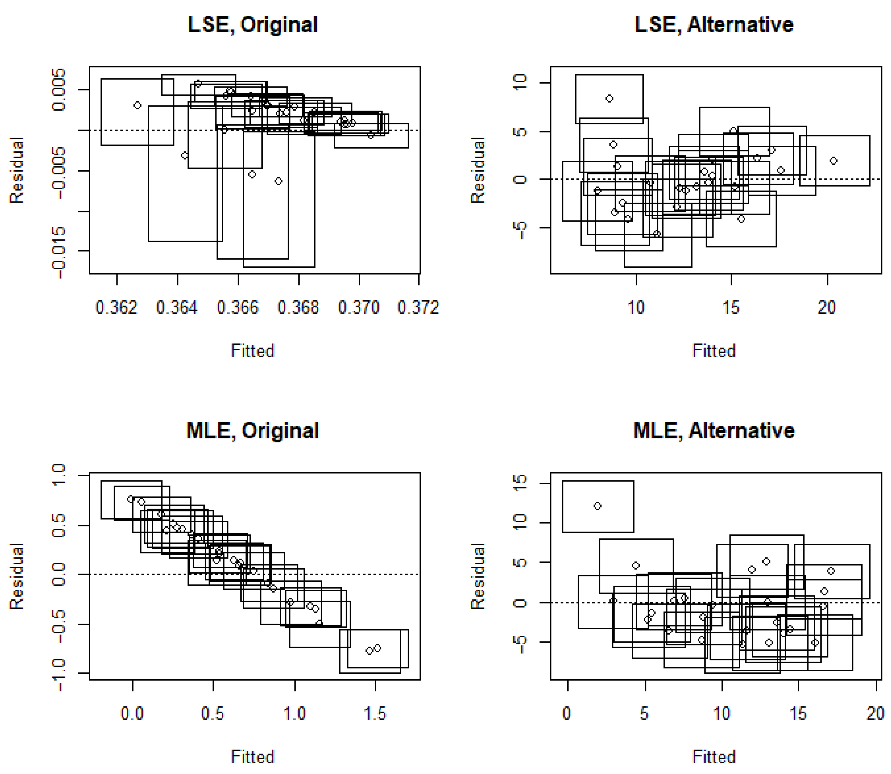The residual plot is shown in Figure 1. In this figure, ‘LSE’ stands for the least-squares estimation, ‘MLE’ stands for the maximum likelihood estimation, ‘Original’ stands for the Box-Cox linear model, and ‘Alternative’ stands for the alternative Box-Cox linear model.

Figure 1 shows that when the fitted model is a Box-Cox linear model, the residual plots of the least-squares estimation and maximum likelihood estimation have obvious deviations. However, when the fitted model is an alternative Box-Cox linear model, the residuals of the two estimates do not deviate from zero or change unevenly. This shows that the least-squares and maximum likelihood estimations suit the uncertain alternative Box-Cox linear models but not the uncertain Box-Cox linear models. In addition, Table 3 shows that when the fitted model is a Box-Cox linear model, the estimated values of $\lambda$ for the least-squares analysis and the maximum likelihood estimation are all relatively small. Note that the problem of underestimation of $\lambda$ in the least-squares estimation of Box-Cox linear model was pointed out in [14]. A similar situation occurred for the maximum likelihood estimation in this numerical experiment.

For the uncertain Box-Cox linear model, a weighted LSE method was proposed by [14]. Table 3 shows that the results of the weighted least-squares estimation method are very similar to that of the direct least-squares after reparameterization. This is because the two estimation methods are equivalent, which we have explained before. Therefore, directly fitting the uncertain alternative Box-Cox linear model without constructing a penalty term can also avoid underestimating $\lambda$. It is more straightforward than [14].

Table 3 shows that when the fitted model is an uncertain alternative Box-Cox model, the results of the least-squares analysis and that of the maximum likelihood estimation are significantly different. Since the residual biases and standard deviations of the least-squares estimation are relatively small, and the estimation process is relatively simple, we recommend using the uncertain least-squares method to estimate the alternative Box-Cox model.

To sum up, such a numerical example shows that, compared with the Box-Cox model, we do not have the problem of underestimated $\lambda$ for the uncertain alternative Box-Cox model. Therefore, the least-squares estimation or the maximum likelihood estimation can be used directly without constructing a weighted estimation method. In addition, for the uncertain alternative Box-Cox model, the least-squares estimation shows better performance in terms of residuals and is therefore recommended.

4.2. Uncertain Michaelis–Menten Kinetics Case

Next, this subsection consider fitting an uncertain Box-Cox Michaelis–Menten kinetics regression model [24]. The imprecise data shown in

Table 4. The imprecise data used to fit the uncertain Box-Cox Michaelis-Menten kinetics regression model, where $\mathcal{L}(a,b)$ is the linear uncertainty variable.

i	1	2	3	4	5	6
${\tilde{x}}_i$	$\mathcal{L}(5,6)$	$\mathcal{L}(5,6)$	$\mathcal{L}(3,4)$	$\mathcal{L}(4,5)$	$\mathcal{L}(5,6)$	$\mathcal{L}(6,7)$
i	7	8	9	10	11	12
${\tilde{x}}_i$	$\mathcal{L}(5,6)$	$\mathcal{L}(6,7)$	$\mathcal{L}(3,4)$	$\mathcal{L}(7,8)$	$\mathcal{L}(4,5)$	$\mathcal{L}(4,5)$
i	13	14	15	16	17	18
${\tilde{x}}_i$	$\mathcal{L}(6,7)$	$\mathcal{L}(6,7)$	$\mathcal{L}(8,9)$	$\mathcal{L}(7,8)$	$\mathcal{L}(6,7)$	$\mathcal{L}(3,4)$
i	19	20	21	22	23	24
${\tilde{x}}_i$	$\mathcal{L}(5,6)$	$\mathcal{L}(4,5)$	$\mathcal{L}(3,4)$	$\mathcal{L}(4,5)$	$\mathcal{L}(4,5)$	$\mathcal{L}(5,6)$

are adopted from the source there.

In this case, this section also applies the LSE and the MLE respectively to fit the original uncertain Michaelis–Menten kinetics regression model and the transformed uncertain Box-Cox Michaelis–Menten kinetics regression model.

The residual graph, as well as the mean and standard deviation of the residuals, remains useful here for residual analysis. The optimization, integration in the LSE and numerical derivation in the MLE are again carried out via the $\mathtt{optim}\left(\right)$ function, the $\mathtt{integrate}$ function and the $\mathtt{fderiv}$ function, respectively. The parameter settings are explored as are those of the previous linear case. Please refer to

Table 5. The initial values of the parameters selected for fitting the uncertain Box-Cox Michaelis–Menten kinetics regression model.

No.	${\mathit{\beta }}_1$	${\mathit{\beta }}_2$	$\mathit{\lambda }$	$\mathit{\sigma }$	No.	${\mathit{\beta }}_1$	${\mathit{\beta }}_2$	$\mathit{\lambda }$	$\mathit{\sigma }$
1	2	2	0	0.5	10	2	2	0.5	1
2	0	0	0.5	0.5	11	2	2	1	1
3	2	2	1	0.5	12	0	0	0	1
4	2	0	0.5	0.5	13	0	2	0	1
5	0	2	1	0.5	14	2	2	0.5	1
6	2	2	0	0.5	15	2	0	1	1
7	0	2	1	0.5	16	2	0	1	1
8	2	0	0	0.5	17	2	2	0	1
9	2	2	0.5	0.5	18	0	2	0.5	1

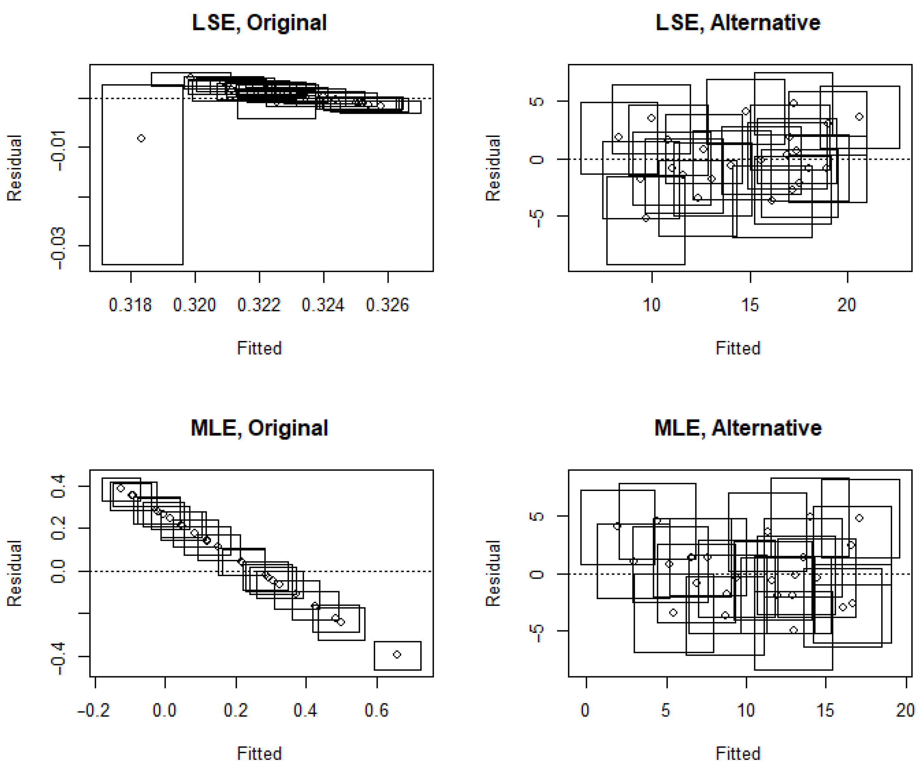
for the parameters details and Table 3 for the results of the parameter estimation with the mean and standard deviation. The residual plot is presented in Figure 2. In this figure, ‘LSE’ stands for the least-squares estimation, ‘MLE’ stands for the maximum likelihood estimation; ‘Original’ stands for the uncertain Box-Cox Michaelis–Menten kinetics regression model, and ‘Alternative’ stands for the alternative uncertain Box-Cox Michaelis–Menten kinetics regression model.

From Figure 2, we can see that for the original uncertain Michaelis–Menten kinetics regression model, there is evident variation in the residual plots from the LSE and the MLE. This is not true for the uncertain alternative Box-Cox Michaelis–Menten kinetics regression model, where the residuals neither deviate from zero nor change unevenly. Therefore, we conclude that the LSE and MLE are both appropriate to use for estimating the uncertain alternative Box-Cox Michaelis–Menten kinetics regression model, but not for the original uncertain Michaelis–Menten kinetics regression models.

Table 6. The estimation results of the uncertain Box-Cox Michaelis–Menten kinetics regression model as well as the mean (Resid. mean) and standard deviation (Resid. sd) of the residuals.

Method	Model	${\mathit{\beta }}_1$	${\mathit{\beta }}_2$	$\mathit{\lambda }$	$\mathit{\sigma }$	Resid. mean	Resid. sd
RLSE	Original	1.3959	5.3682	2.0315	-	0.2643	1.5360
LSE	Original	0.0019	0.3167	−2.5421	-	0.0000	1.4704
LSE	Alternative	8.2893	3.1876	2.0316	-	0.0008	3.1312
LSE	Transformed	1.3959	5.3682	2.0316	-	0.2643	1.5360
MLE	Original	0.0129	0.0012	−3.3220	0.2124	0.1132	0.1421
MLE	Alternative	3.4232	0.3681	1.2561	1.3327	0.2781	4.3663
MLE	Transformed	3.4336	0.3681	1.2561	1.3327	0.2781	3.3663

shows the estimation results of the uncertain Box-Cox Michaelis–Menten kinetics regression model as well as the mean (Resid. mean) and standard deviation (Resid. sd) of the residuals. In this table, ‘RLSE’ stands for the weighted least-squares method from [14], ‘LSE’ stands for the least-squares estimation, and ‘MLE’ stands for the maximum likelihood estimation. ‘Original’ means that the fitted model is a Box-Cox model, ‘Alternative’ means that the fitted model is an alternative Box-Cox model, and ‘Transformed’ means that after fitting the alternative Box-Cox model, the estimation results are reparameterized to be compared with that of the Box-Cox model. Table 6 offers evidence that when the original uncertain Michaelis–Menten kinetics regression model is used, both LSE and MLE are inclined to conspicuously underestimate $\lambda$, which is a persisting issue pointed out in [14]. On the contrary, Table 6 supports the uncertain alternative Box-Cox Michaelis–Menten kinetics regression model, with distinct LSE and MLE results.

Due to the user-friendliness and small-scale residual biases and standard deviations, the alternative Box-Cox Michaelis–Menten kinetics regression model using uncertain LSE to estimate parameters should be advocated.

The weighted least-squares estimation method proposed by [14] for the uncertain Box-Cox Michaelis–Menten kinetics regression model is also inspected. It turns out that the corresponding results shown in Table 6 are pretty close to those from the direct least-squares after reparameterization, which verifies our claim on the equivalence of the two estimation methods. As a result, the uncertain alternative Box-Cox Michaelis–Menten kinetics regression model for the simplicity of directly fitting deserves to be recommended, with no need for penalty terms and without concerns of underestimated $\lambda$.

In conclusion, a thorough comparison between the uncertain Box-Cox Michaelis–Menten kinetics regression model and the uncertain alternative Box-Cox Michaelis–Menten kinetics regression model favors the latter. Both LSE and MLE perform well in the latter case, with no need for a weighted procedure. As far as LSE and MLE are compared in the latter case, LSE stands out.

5. Conclusions and Discussion

This article proposed an alternative Box-Cox model, gave its least-squares estimation and maximum likelihood estimation, and compared its performance with previous estimation methods. Parameter estimation was realized mainly by minimizing the Euclidean distance between the response variables $H(y;\lambda )$(after transformation) and the corresponding fitted values $f(x_1,x_2,\cdots ,x_p|\beta )$.

There are theoretical issues mentioned in the literature [14] that state that when f is a linear function of $x_1,x_2,\cdots ,x_p$ and all $Y_i$ are greater than 1, this distance approaches zero as $\lambda \to -\infty$ and $\beta =0$. In the numerical simulations above, the upper and lower bounds of $\lambda$ were used to avoid this problem. However, the cross-validation results showed that the estimated value of $\lambda$ could remain unsatisfactorily low. Therefore, regarding this issue, this article introduced a penalty term on $\lambda$ for MLE and proposed an uncertain alternative Box-Cox model to improve the estimation. In addition, a residual graph method was proposed to evaluate the validity of the fitting uncertainty model. It turns out that the residuals become symmetric about the origin, which is desirable in applications of experts’ experimental data. Our work enriches the theoretical framework of uncertain regression, providing effective analytical evaluation methods for a large class of flexible uncertain regression analysis, especially on nonlinear uncertain Box-Cox models. This paper has value in analyzing uncertain data, such as experts’ experimental data in terms of theories and applications. Later on, we plan to test the significance of regression coefficients in some uncertain regression models, exploring ways to compare and analyze the differences between the uncertain significance tests and the statistical significance tests.