On the Interpretation of the Balance Function

Abstract

We construct a simple toy model and explicitly demonstrate that the balance function (BF) can become negative for some values of the rapidity separation and hence cannot have any probabilistic interpretation. In particular, the BF cannot be interpreted as the probability density for the balancing charges to occur separated by the given rapidity interval.

1. Introduction

The net charge event-by-event fluctuations are considered as indicators of the formation of a quark gluon plasma (QGP) in ultrarelativistic heavy ion collisions [1,2,3,4,5]. To characterize numerically the magnitude of these fluctuations, one usually uses the so-called D measure:

$$D=4\frac{D_Q}{⟨n⟩}=4{\omega }_Q$$

(1)

which provides a measure of the net charge fluctuations per unit entropy. Here, $D_Q$ and ${\omega }_Q=D_Q/⟨n⟩$ are the variance and reduced variance of the net charge, $Q=n_{+}-n_{-}$, $n=n_{+}+n_{-}$. The $n^{+}$ and $n^{-}$ are the number of positive and negative particles observed in some acceptance window, e.g., in some pseudorapidity interval $\delta \eta$.

The net charge fluctuations were estimated using various theoretical approaches with the general conclusion that the hadronization of QGP should lead to a final state characterized by a sharp decrease in the net charge fluctuations in comparison with hadronic gas (HG). For example, in the article [1], it was shown that in a simple model, if we neglect quark–quark interactions, the D turns out to be about 4 times less for QGP than for HG (see further discussion of this topic in [4,5]).

In modern experiments, net charge fluctuations are usually studied [3,4,5] by calculating the so-called dynamic fluctuation variable ${\nu }_{dyn}$, defined as:

$${\nu }_{dyn}\left(\delta \eta \right)\equiv \frac{⟨n_{+}(n_{+}-1)⟩}{{⟨n_{+}⟩}^2}+\frac{⟨n_{-}(n_{-}-1)⟩}{{⟨n_{-}⟩}^2}-2\frac{⟨n_{+}{n}_{-}⟩}{⟨n_{+}⟩⟨n_{-}⟩}.$$

(2)

This variable is simply connected with the D measure [4,5]:

$$D=⟨n⟩{\nu }_{dyn}\left(\delta \eta \right)+4$$

(3)

In some cases, it is more convenient to modify the normalization of the dynamic fluctuation variable ${\nu }_{dyn}$ by introducing

$${\nu }_s\left(\delta \eta \right)\equiv -\frac{1}{1/⟨n_{+}⟩+1/⟨n_{-}⟩}{\nu }_{dyn}\left(\delta \eta \right)$$

(4)

(see Formula (3) in [6]). This variable is closely connected with the so-called balance function (BF) [7], usually defined as

$$B({\eta }_1,{\eta }_2)=\frac{1}{2}\left[\frac{{\rho }_{+-}({\eta }_1,{\eta }_2)}{{\rho }_{+}\left({\eta }_1\right)}+\frac{{\rho }_{-+}({\eta }_1,{\eta }_2)}{{\rho }_{-}\left({\eta }_1\right)}-\frac{{\rho }_{++}({\eta }_1,{\eta }_2)}{{\rho }_{+}\left({\eta }_1\right)}-\frac{{\rho }_{--}({\eta }_1,{\eta }_2)}{{\rho }_{-}\left({\eta }_1\right)}\right],$$

(5)

where ${\rho }_{+}\left(\eta \right)$, ${\rho }_{+-}({\eta }_1,{\eta }_2)$, etc., are the inclusive and double inclusive pseudorapidity distributions of corresponding charged particles (for the correspondence with other possible alternative definitions of the BF see, e.g., [8]).

The relationship between the ${\nu }_s\left(\delta \eta \right)$ and the $B({\eta }_1,{\eta }_2)$ in the simplest way can be established in the mid-rapidity region at LHC energies, where the translation invariance in rapidity is valid. In this case the single inclusive distributions are constant: ${\rho }_{+}\left(\eta \right)=⟨n_{+}⟩/\delta \eta \equiv {\rho }_{+}^0$, ${\rho }_{-}\left(\eta \right)=⟨n_{-}⟩/\delta \eta \equiv {\rho }_{-}^0$ and the double inclusive distributions depend only on the differences of their arguments: ${\rho }_{+-}({\eta }_1,{\eta }_2)={\rho }_{+-}({\eta }_1-{\eta }_2)$, etc. Hence, the BF also will depend only on the ${\eta }_1-{\eta }_2\equiv \mathsf{\Delta }\eta$.

The charge symmetry is also well satisfied for this case, ${\rho }_{+}^0={\rho }_{-}^0$, and

$$⟨n_{+}⟩=⟨n_{-}⟩=⟨n⟩/2,{\omega }_{n_{+}}={\omega }_{n_{-}},{\omega }_{n_{+}}\equiv D_{n_{+}}/⟨n_{+}⟩,D_{n_{+}}\equiv ⟨n_{+}^2⟩-{⟨n_{+}⟩}^2.$$

(6)

Then, the expressions (4) for ${\nu }_s\left(\delta \eta \right)$ and (5) for $B({\eta }_1,{\eta }_2)$ are reduced to

$${\nu }_s\left(\delta \eta \right)=-\frac{⟨n⟩}{4}{\nu }_{dyn}\left(\delta \eta \right)=\frac{⟨n_{+}{n}_{-}⟩-⟨n_{+}(n_{+}-1)⟩}{⟨n_{+}⟩}=1+\frac{⟨n_{+}{n}_{-}⟩-⟨n_{+}^2⟩}{⟨n_{+}⟩}$$

(7)

(see Formula (4) in [6]) and

$$B({\eta }_1-{\eta }_2)=\frac{{\rho }_{+-}({\eta }_1-{\eta }_2)-{\rho }_{++}({\eta }_1-{\eta }_2)}{{\rho }_{+}^0}.$$

(8)

Then, by the direct integration of (8) we get

$${\nu }_s\left(\delta \eta \right)=\frac{1}{\delta \eta }{\int }_{\delta \eta }d{\eta }_1{\int }_{\delta \eta }d{\eta }_{2}B({\eta }_1-{\eta }_2),$$

(9)

where we have taken into account the normalization conditions (15) and (16) (see the next section).

Since, by the definition (5), the BF is symmetric: $B\left(\mathsf{\Delta }\eta \right)=B(-\mathsf{\Delta }\eta )$, the integral (9) can be written as follows (see, e.g., Appendix A in the paper [9]):

$$\begin{array}{ll}{\nu }_s\left(\delta \eta \right)& =\frac{1}{\delta \eta }{\int }_{\eta }^{\eta +\delta \eta }d{\eta }_1{\int }_{\eta }^{\eta +\delta \eta }d{\eta }_{2}B({\eta }_1-{\eta }_2)=\frac{1}{\delta \eta }{\int }_{-\delta \eta /2}^{\delta \eta /2}d{\eta }_1{\int }_{-\delta \eta /2}^{\delta \eta /2}d{\eta }_{2}B({\eta }_1-{\eta }_2)\\ & =\frac{1}{\delta \eta }{\int }_{-\delta \eta }^{\delta \eta }d\left(\mathsf{\Delta }\eta \right)B\left(\mathsf{\Delta }\eta \right)t_{\delta \eta }\left(\mathsf{\Delta }\eta \right)=\frac{2}{\delta \eta }{\int }_0^{\delta \eta }d\left(\mathsf{\Delta }\eta \right)B\left(\mathsf{\Delta }\eta \right)(\delta \eta -\mathsf{\Delta }\eta ),\end{array}$$

(10)

where the $t_{\delta \eta }\left(\mathsf{\Delta }\eta \right)$ is the usual phase space “triangular” weight function:

$$t_{\delta \eta }\left(\mathsf{\Delta }\eta \right)=[\theta (-\mathsf{\Delta }\eta )(\delta \eta +\mathsf{\Delta }\eta )+\theta \left(\mathsf{\Delta }\eta \right)(\delta \eta -y)]\theta (\delta \eta -|\mathsf{\Delta }\eta \left|\right)\ge 0$$

(11)

(see Figure A.1 in the paper [9]).

In paper [7], the authors state that “The BF would represent the probability that the balancing charges were separated by $\mathsf{\Delta }\eta$ (in our formalism we include a division by $\mathsf{\Delta }\eta$ to express $B\left(\mathsf{\Delta }\eta \right)$ as a density)”. Nevertheless, in the Introduction of the paper [5], it is mentioned that the value of ${\nu }_{dyn}\left(\delta \eta \right)$ can be both negative and positive: “A negative value of ${\nu }_{dyn}$ signifies the dominant contribution from correlations between pairs of opposite charges. On the other hand, a positive value indicates the significance of the same charge pair correlations”.

By Formula (4), this means that in some cases the ${\nu }_s\left(\delta \eta \right)$ can take negative values. Then, by Formula (10), we see that in this case the BF must also be negative at least at some values of $\mathsf{\Delta }\eta$ to ensure the negative value of the integral (10), as the triangular weight function (11) is positive: $t_{\delta \eta }\left(\mathsf{\Delta }\eta \right)\ge 0$. However, if the ${\nu }_s\left(\delta \eta \right)$ and the BF $B\left(\mathsf{\Delta }\eta \right)$ can take negative values they cannot have any probabilistic interpretation, in particular that mentioned in the paper [7].

In the present short note we explicitly confirm this fact by direct calculations for a very simple toy model.

Note also that the ${\nu }_s\left(\delta \eta \right)$ is simply connected with the so-called strongly intensive variable [10,11], $\mathsf{\Sigma }(n_{+},n_{-})$,

$${\nu }_s\left(\delta \eta \right)=1-\mathsf{\Sigma }(n_{+},n_{-}),$$

(12)

analyzed earlier in [12] as $\mathsf{\Sigma }(n_F^{+},n_F^{-})$.

2. General Definitions and Relations

We start with the definitions of inclusive and double inclusive pseudorapidity distributions of charged particles:

$${\rho }_{\pm }\left(\eta \right)\equiv \frac{d{N}_{ch}^{\pm }}{d\eta },{\rho }_{++}({\eta }_1,{\eta }_2)\equiv \frac{d^2{N}_{ch}^{++}}{d{\eta }_{1}d{\eta }_2},{\rho }_{+-}({\eta }_1,{\eta }_2)\equiv \frac{d^2{N}_{ch}^{+-}}{d{\eta }_{1}d{\eta }_2},$$

(13)

which are normalized as follows:

$${\int }_{\delta \eta }d\eta {\rho }_{\pm }\left(\eta \right)=⟨n_{\pm }⟩,$$

(14)

$${\int }_{\delta \eta }d{\eta }_1{\int }_{\delta \eta }d{\eta }_2{\rho }_{++}({\eta }_1,{\eta }_2)=⟨n_{+}(n_{+}-1)⟩.$$

(15)

$${\int }_{\delta \eta }d{\eta }_1{\int }_{\delta \eta }d{\eta }_2{\rho }_{+-}({\eta }_1,{\eta }_2)=⟨n_{+}{n}_{-}⟩.$$

(16)

Then, we define the two-particle correlation functions in a standard way [3]:

$$C_{++}({\eta }_1,{\eta }_2)\equiv \frac{{\rho }_{++}({\eta }_1,{\eta }_2)}{{\rho }_{+}\left({\eta }_1\right){\rho }_{+}\left({\eta }_2\right)}-1,C_{+-}({\eta }_1,{\eta }_2)\equiv \frac{{\rho }_{+-}({\eta }_1,{\eta }_2)}{{\rho }_{+}\left({\eta }_1\right){\rho }_{-}\left({\eta }_2\right)}-1.$$

(17)

In the mid-rapidity region at LHC energies, when the translation invariance in rapidity and the charge symmetry, mentioned above, take place, these formulae can be simplified, using that

$${\rho }_{+}\left(\eta \right)={\rho }_{-}\left(\eta \right)={\rho }_{+}^0=const=⟨n_{+}⟩/\delta \eta ,$$

(18)

$${\rho }_{++}({\eta }_1,{\eta }_2)={\rho }_{++}({\eta }_1-{\eta }_2),{\rho }_{+-}({\eta }_1,{\eta }_2)={\rho }_{+-}({\eta }_1-{\eta }_2)$$

and hence

$$C_{++}({\eta }_1,{\eta }_2)=C_{++}({\eta }_1-{\eta }_2),C_{+-}({\eta }_1,{\eta }_2)=C_{+-}({\eta }_1-{\eta }_2).$$

(19)

Then, by (14)–(19), we have

$${\rho }_{+}^0{\rho }_{+}^0{\int }_{\delta \eta }d{\eta }_1{\int }_{\delta \eta }d{\eta }_2{C}_{++}({\eta }_1-{\eta }_2)=⟨n_{+}(n_{+}-1)⟩-{⟨n_{+}⟩}^2.$$

(20)

$${\rho }_{+}^0{\rho }_{-}^0{\int }_{\delta \eta }d{\eta }_1{\int }_{\delta \eta }d{\eta }_2{C}_{+-}({\eta }_1-{\eta }_2)=⟨n_{+}{n}_{-}⟩-⟨n_{+}⟩⟨n_{-}⟩.$$

(21)

Using definition (7), we express the ${\nu }_s\left(\delta \eta \right)$ through the correlation functions $C_{+-}$ and $C_{++}$ in the model independent way:

$${\nu }_s\left(\delta \eta \right)=\frac{{\rho }_{+}^0}{\delta \eta }{\int }_{\delta \eta }d{\eta }_1{\int }_{\delta \eta }d{\eta }_2\left[C_{+-}({\eta }_1-{\eta }_2)-C_{++}({\eta }_1-{\eta }_2)\right].$$

(22)

Simultaneously, from Formula (8) for the BF, we have

$$B({\eta }_1-{\eta }_2)={\rho }_{+}^0·\left[C_{+-}({\eta }_1-{\eta }_2)-C_{++}({\eta }_1-{\eta }_2)\right].$$

(23)

3. The Models with Independent Identical Sources

In models with independent identical sources, the following formula [9] for $C({\eta }_1,{\eta }_2)$ takes place (see a simple proof in Appendix A):

$$C({\eta }_1,{\eta }_2)=\frac{\mathsf{\Lambda }({\eta }_1,{\eta }_2)+{\omega }_N}{⟨N⟩},$$

(24)

where N is a number of sources, which fluctuates event by event around some mean value, $⟨N⟩$, with some scaled variance, ${\omega }_N=D_N/⟨N⟩$.

The $\mathsf{\Lambda }({\eta }_1,{\eta }_2)$ is the two-particle correlation function characterizing a single source. It is defined similarly to $C({\eta }_1,{\eta }_2)$, but takes into account only particles produced by a given source:

$${\mathsf{\Lambda }}_{++}({\eta }_1,{\eta }_2)\equiv \frac{{\lambda }_{++}({\eta }_1,{\eta }_2)}{{\lambda }_{+}\left({\eta }_1\right){\lambda }_{+}\left({\eta }_2\right)}-1,{\mathsf{\Lambda }}_{+-}({\eta }_1,{\eta }_2)\equiv \frac{{\lambda }_{+-}({\eta }_1,{\eta }_2)}{{\lambda }_{+}\left({\eta }_1\right){\lambda }_{-}\left({\eta }_2\right)}-1,$$

(25)

where

$${\lambda }_{\pm }\left(\eta \right)\equiv \frac{d{N}_{ch}^{\pm }}{d\eta },{\lambda }_{++}({\eta }_1,{\eta }_2)\equiv \frac{d^2{N}_{ch}^{++}}{d{\eta }_{1}d{\eta }_2},{\lambda }_{+-}({\eta }_1,{\eta }_2)\equiv \frac{d^2{N}_{ch}^{+-}}{d{\eta }_{1}d{\eta }_2},$$

(26)

are inclusive and double inclusive pseudorapidity distributions of charged particles produced by a given source. They are normalized as follows:

$${\int }_{\delta \eta }d\eta {\lambda }_{\pm }\left(\eta \right)=⟨{\mu }_{\pm }⟩,$$

(27)

$${\int }_{\delta \eta }d{\eta }_1{\int }_{\delta \eta }d{\eta }_2{\lambda }_{++}({\eta }_1,{\eta }_2)=⟨{\mu }_{+}({\mu }_{+}-1)⟩.$$

(28)

$${\int }_{\delta \eta }d{\eta }_1{\int }_{\delta \eta }d{\eta }_2{\lambda }_{+-}({\eta }_1,{\eta }_2)=⟨{\mu }_{+}{\mu }_{-}⟩.$$

(29)

In the mid-rapidity region at LHC energies, when the translation invariance in rapidity and the charge symmetry take place, these formulae can again be simplified, using that

$${\lambda }_{+}\left(\eta \right)={\lambda }_{-}\left(\eta \right)={\lambda }_{+}^0={\lambda }_{-}^0=const=\frac{⟨{\mu }_{+}⟩}{\delta \eta }=\frac{⟨n_{+}⟩}{\delta \eta ⟨N⟩}=\frac{{\rho }_{+}^0}{⟨N⟩},$$

(30)

$${\lambda }_{++}({\eta }_1,{\eta }_2)={\lambda }_{++}({\eta }_1-{\eta }_2),{\lambda }_{+-}({\eta }_1,{\eta }_2)={\lambda }_{+-}({\eta }_1-{\eta }_2)$$

and hence

$${\mathsf{\Lambda }}_{++}({\eta }_1,{\eta }_2)={\mathsf{\Lambda }}_{++}({\eta }_1-{\eta }_2),{\mathsf{\Lambda }}_{+-}({\eta }_1,{\eta }_2)={\mathsf{\Lambda }}_{+-}({\eta }_1-{\eta }_2).$$

(31)

Then,

$${\mathsf{\Lambda }}_{++}({\eta }_1-{\eta }_2)=\frac{{\lambda }_{++}({\eta }_1-{\eta }_2)}{{\lambda }_{+}^0{\lambda }_{+}^0}-1,{\mathsf{\Lambda }}_{+-}({\eta }_1-{\eta }_2)=\frac{{\lambda }_{+-}({\eta }_1-{\eta }_2)}{{\lambda }_{+}^0{\lambda }_{-}^0}-1.$$

(32)

Substituting the general connection (24) into Formula (22), we finally express the ${\nu }_s\left(\delta \eta \right)$ through the correlation functions ${\mathsf{\Lambda }}_{+-}$ and ${\mathsf{\Lambda }}_{++}$ of a single source:

$${\nu }_s\left(\delta \eta \right)=\frac{{\lambda }_{+}^0}{\delta \eta }{\int }_{\delta \eta }d{\eta }_1{\int }_{\delta \eta }d{\eta }_2\left[{\mathsf{\Lambda }}_{+-}({\eta }_1-{\eta }_2)-{\mathsf{\Lambda }}_{++}({\eta }_1-{\eta }_2)\right].$$

(33)

Note that a dependence on $⟨N⟩$ and ${\omega }_N=D_N/⟨N⟩$ is canceled which proves the strongly intensive behavior of this variable in the case with identical sources.

We also see this from the fact that Formula (33) coincides with the definition (7) when replacing all engaged quantities with the corresponding ones for one source. That also can be written as

$${\nu }_s\left(\delta \eta \right)=\frac{⟨n_{+}{n}_{-}⟩-⟨n_{+}(n_{+}-1)⟩}{⟨n_{+}⟩}=\frac{⟨{\mu }_{+}{\mu }_{-}⟩-⟨{\mu }_{+}({\mu }_{+}-1)⟩}{⟨{\mu }_{+}⟩}$$

(34)

in any model with identical courses.

As mentioned in the Introduction, the ${\nu }_s\left(\delta \eta \right)$ is simply connected with the balance function $B({\eta }_1-{\eta }_2)$. In any model with identical independent sources in the central region, where the translation invariance in rapidity and the charge symmetry take place, we have (see, e.g., Section 5 of the paper [8]):

$$B({\eta }_1-{\eta }_2)={\lambda }_{+}^0·\left[{\mathsf{\Lambda }}_{+-}({\eta }_1-{\eta }_2)-{\mathsf{\Lambda }}_{++}({\eta }_1-{\eta }_2)\right].$$

(35)

One can immediately obtain this formula by substituting (24) into (23) and taking into account the relation (30).

Comparing Formulae (33) and (35), we see that the general relation (9)

$${\nu }_s\left(\delta \eta \right)=\frac{1}{\delta \eta }{\int }_{\delta \eta }d{\eta }_1{\int }_{\delta \eta }d{\eta }_{2}B({\eta }_1-{\eta }_2),$$

of course, is true in this particular case.

4. Toy Models with Sources Emitting Particles Uniformly Distributed in Rapidity

Let us consider at first a very simple model, when each source always produces only one plus–minus pair, with plus and minus particles being uniformly distributed in some wide interval $(-Y/2,Y/2)$, $Y\gg 1$.

In this simple model,

$${\lambda }_{+}^0=\frac{1}{Y},{\lambda }_{++}({\eta }_1-{\eta }_2)=0,{\lambda }_{+-}({\eta }_1-{\eta }_2)=\frac{1}{Y^2}.$$

(36)

To test these formulae we can use the normalization conditions (27)–(29) in the whole acceptance Y:

$${\int }_{Y}d\eta {\lambda }_{\pm }\left(\eta \right)=1,$$

(37)

$${\int }_{Y}d{\eta }_1{\int }_{Y}d{\eta }_2{\lambda }_{++}({\eta }_1-{\eta }_2)=0.$$

(38)

$${\int }_{Y}d{\eta }_1{\int }_{Y}d{\eta }_2{\lambda }_{+-}({\eta }_1-{\eta }_2)=1.$$

(39)

Then, by (32), we have

$${\mathsf{\Lambda }}_{++}({\eta }_1-{\eta }_2)=-1,{\mathsf{\Lambda }}_{+-}({\eta }_1-{\eta }_2)=0.$$

(40)

As expected, we see no correlation between plus and minus particles produced from the same source, ${\mathsf{\Lambda }}_{+-}({\eta }_1-{\eta }_2)=0$, and a strong anticorrelation between plus and plus particles from one source, ${\mathsf{\Lambda }}_{++}({\eta }_1-{\eta }_2)=-1$, because the only plus particle, produced from a source, cannot be simultaneously at both ${\eta }_1$ and ${\eta }_2$ pseudorapidities.

Substituting all this into Formula (33), we find

$${\nu }_s\left(\delta \eta \right)=\frac{1}{Y\delta \eta }\delta {\eta }^2\left[0-(-1)\right]=\frac{\delta \eta }{Y}.$$

(41)

The interpretation of the ${\nu }_s\left(\delta \eta \right)=\frac{\delta \eta }{Y}$ as the probability to find the negatively charged particle in the rapidity interval $\delta \eta$ under the condition that we already have the positively charged particle in this interval looks very suspicious. This is because, as we can see from Formulae (40) and (41), this result arises not due to correlation between plus and minus particles but due to a strong anticorrelation between plus and plus particles in this simple model.

To verify these suspicions, let us consider a more sophisticated model, when each source always produces two plus–minus pairs, with two plus and two minus particles being uniformly distributed in some wide interval $(-Y/2,Y/2)$, $Y\gg 1$.

In this version of the model,

$${\lambda }_{+}^0=\frac{2}{Y},{\lambda }_{++}({\eta }_1-{\eta }_2)=\frac{2}{Y^2},{\lambda }_{+-}({\eta }_1-{\eta }_2)=\frac{4}{Y^2}.$$

(42)

Again, we can test these formulae using the normalization conditions (27)–(29) in the whole acceptance Y:

$${\int }_{Y}d\eta {\lambda }_{\pm }\left(\eta \right)=2,$$

(43)

$${\int }_{Y}d{\eta }_1{\int }_{Y}d{\eta }_2{\lambda }_{++}({\eta }_1-{\eta }_2)=2.$$

(44)

$${\int }_{Y}d{\eta }_1{\int }_{Y}d{\eta }_2{\lambda }_{+-}({\eta }_1-{\eta }_2)=4.$$

(45)

Then, by (32), we have

$${\mathsf{\Lambda }}_{++}({\eta }_1-{\eta }_2)=-\frac{1}{2},{\mathsf{\Lambda }}_{+-}({\eta }_1-{\eta }_2)=0.$$

(46)

As expected, again, we see no correlation between plus and minus particles produced from the same source, ${\mathsf{\Lambda }}_{+-}({\eta }_1-{\eta }_2)=0$, and attenuation of the anticorrelation between plus and plus particles from one source, ${\mathsf{\Lambda }}_{++}({\eta }_1-{\eta }_2)=-\frac{1}{2}$, because now two plus particles are produced from a source and ${\lambda }_{++}({\eta }_1-{\eta }_2)=\frac{2}{Y^2}>0$.

Substituting all this into Formula (33), we find that, again,

$${\nu }_s\left(\delta \eta \right)=\frac{2}{Y\delta \eta }\delta {\eta }^2\left[0-\left(-\frac{1}{2}\right)\right]=\frac{\delta \eta }{Y}.$$

(47)

It is easy to prove that in the model, when each source always produces k plus–minus pairs, with k plus and k minus particles being uniformly distributed in some wide interval $(-Y/2,Y/2)$, $Y\gg 1$, we have

$${\nu }_s\left(\delta \eta \right)=\frac{k}{Y\delta \eta }\delta {\eta }^2\left[0-\left(-\frac{1}{k}\right)\right]=\frac{\delta \eta }{Y}.$$

(48)

The interpretation of the ${\nu }_s\left(\delta \eta \right)=\frac{\delta \eta }{Y}$ as the probability to find the negatively charged particle in the rapidity interval $\delta \eta$ under the condition that we already have the positively charged particle in this interval still holds, since in each event we have an equal number of plus and minus particles uniformly distributed in some wide interval $(-Y/2,Y/2)$, $Y\gg 1$, as in the initial version of the model with one charge pair production by a source. Nevertheless, it looks strange since it based not on correlations between plus and minus particles but on anticorrelations between plus and plus particles in this simple model.

Note that, in this case, by Formula (35), the BF ("the probability density") is equal to $1/Y$:

$$B\left(\mathsf{\Delta }\eta \right)=\frac{k}{Y}\left[0-\left(-\frac{1}{k}\right)\right]=\frac{1}{Y},$$

(49)

which after integration over rapidity interval $\delta \eta$ by (10) again leads to Formula (48).

5. Toy Model with Production of Correlated Charge Pairs by a Source

As we can see in the previous section, this result, ${\nu }_s\left(\delta \eta \right)=\frac{\delta \eta }{Y}$, arises due to plus–plus anticorrelation, ${\mathsf{\Lambda }}_{++}({\eta }_1-{\eta }_2)=-\frac{1}{k}$, in the version of the model with the production of k independent plus–minus pairs by each source. After multiplying by ${\lambda }_{+}^0=\frac{k}{Y}$ and the integration, we just have this result.

So, in the present section we are trying to introduce some additional plus–plus correlation, formulating a more complex version of the model.

5.1. Strict Correlation between Identical Charges from a Source

Let us consider at first the model in which each source always produces two plus–minus pairs, so that the rapidities of both positive particles coincide and the same is true for both minus particles (the maximally strong correlation between identical charges), whereas the rapidities of the plus pair and the minus pair themselves are uniformly distributed in some wide interval $(-Y/2,Y/2)$, $Y\gg 1$.

In this version of the model,

$${\lambda }_{+}^0=\frac{2}{Y},{\lambda }_{++}({\eta }_1-{\eta }_2)=\frac{2}{Y}\delta ({\eta }_1-{\eta }_2),{\lambda }_{+-}({\eta }_1-{\eta }_2)=\frac{4}{Y^2}.$$

(50)

Again, we can test these formulae using the normalization conditions (27)–(29) in the whole acceptance Y:

$${\int }_{Y}d\eta {\lambda }_{\pm }\left(\eta \right)=2,$$

(51)

$${\int }_{Y}d{\eta }_1{\int }_{Y}d{\eta }_2{\lambda }_{++}({\eta }_1-{\eta }_2)=2.$$

(52)

$${\int }_{Y}d{\eta }_1{\int }_{Y}d{\eta }_2{\lambda }_{+-}({\eta }_1-{\eta }_2)=4.$$

(53)

Then, by (32) we have

$${\mathsf{\Lambda }}_{++}({\eta }_1-{\eta }_2)=\frac{Y}{2}\delta ({\eta }_1-{\eta }_2)-1,{\mathsf{\Lambda }}_{+-}({\eta }_1-{\eta }_2)=0.$$

(54)

As expected, we see again no correlation between plus and minus particles produced from the same source, but we see now strong additional $\frac{Y}{2}\delta ({\eta }_1-{\eta }_2)$ correlation between positive particles from one source.

Substituting all this into Formula (33), we find

$${\nu }_s\left(\delta \eta \right)=\frac{2}{Y\delta \eta }\left[0·\delta {\eta }^2-\left(\frac{Y}{2}·\delta \eta -1·\delta {\eta }^2\right)\right]=\frac{2\delta \eta }{Y}-1.$$

(55)

In Appendix B, we verify this important result using the simple Formula (34).

In conclusion, we see that although for the whole interval at $\delta \eta =Y$ we have ${\nu }_s\left(Y\right)=1$, as expected, nevertheless, the value of the ${\nu }_s\left(\delta \eta \right)$ at $\delta \eta <Y/2$ becomes negative and therefore cannot have any probabilistic interpretation. Note that by Formula (35), the BF in this case looks like this

$$B\left(\mathsf{\Delta }\eta \right)=-\delta \left(\mathsf{\Delta }\eta \right)+\frac{2}{Y},$$

(56)

which after the integration over the rapidity interval $\delta \eta$ by (10) again leads to Formula (A9).

5.2. Soft Correlation between Identical Charges from a Source

From the model construction, it is clear that if we use, instead of the $\delta$-function, any narrow enough distribution normalized by unity, we arrive at the same conclusion. Let us use in this subsection, instead of the $\delta$-function, the step distribution normalized to unity and spread over the interval from $-a$ to a ($a>0$):

$$\delta \left(\mathsf{\Delta }\eta \right)\to h_a\left(\mathsf{\Delta }\eta \right)\equiv \frac{1}{2a}\theta (a-|\mathsf{\Delta }\eta \left|\right),$$

(57)

In this case, for the version of the model described in the previous Section 5.1, we have

$${\lambda }_{+}^0=\frac{2}{Y},{\lambda }_{++}({\eta }_1-{\eta }_2)=\frac{2}{Y-a/2}{h}_a({\eta }_1-{\eta }_2),{\lambda }_{+-}({\eta }_1-{\eta }_2)=\frac{4}{Y^2}.$$

(58)

Using Formula (10), we can check that the factor $2/(Y-a/2)$ ensures the correct normalization condition (28) for the ${\lambda }_{++}({\eta }_1-{\eta }_2)$:

$${\int }_{Y}d\eta {\lambda }_{\pm }\left(\eta \right)=2,$$

(59)

$${\int }_{Y}d{\eta }_1{\int }_{Y}d{\eta }_2{\lambda }_{++}({\eta }_1-{\eta }_2)=$$

(60)

$$={\int }_{-Y/2}^{Y/2}d{\eta }_1{\int }_{-Y/2}^{Y/2}d{\eta }_2{\lambda }_{++}({\eta }_1-{\eta }_2)=\frac{2}{Y-a/2}{\int }_{-Y}^{Y}d\left(\mathsf{\Delta }\eta \right)h_a\left(\mathsf{\Delta }\eta \right)t_Y\left(\mathsf{\Delta }\eta \right)=2,$$

$${\int }_{Y}d{\eta }_1{\int }_{Y}d{\eta }_2{\lambda }_{+-}({\eta }_1-{\eta }_2)=4.$$

(61)

Then, by (32), we have

$${\mathsf{\Lambda }}_{++}({\eta }_1-{\eta }_2)=\frac{Y^2}{2Y-a}{h}_a({\eta }_1-{\eta }_2)-1,{\mathsf{\Lambda }}_{+-}({\eta }_1-{\eta }_2)=0.$$

(62)

By Formula (35), we find now the BF (see Figure 1):

$$B\left(\mathsf{\Delta }\eta \right)=-\frac{Y}{Y-a/2}{h}_a\left(\mathsf{\Delta }\eta \right)+\frac{2}{Y}.$$

(63)

For $\left|\mathsf{\Delta }\eta \right|<a$ by (57), we have

$$B\left(\mathsf{\Delta }\eta \right)=-\frac{Y}{(2Y-a)a}+\frac{2}{Y}.$$

(64)

It is easy to check that at $\left|\mathsf{\Delta }\eta \right|<a<(1-1/\sqrt{2})Y\approx 0.29Y$ the BF is negative, $B\left(\mathsf{\Delta }\eta \right)<0$, and cannot be interpreted as a probability density (see Figure 1, plotted for $Y=10$).

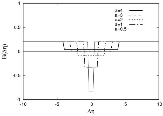
Figure 1. The balance function, $B\left(\mathsf{\Delta }\eta \right)$ (5), as a function of a rapidity distance, $\mathsf{\Delta }\eta$, between observed particles in the toy model with soft correlation between identical charges, considered in Section 5.2. The results are presented for the rapidity interval (−5, 5), $Y=10$, and various values of the model parameter a, characterizing the correlation length between identical charges (see Formula (57) in the text), a = 4 (thick lines), a = 3 (dashed lines), a = 2 (dotted lines), a = 1 (dashed-dotted lines), and a = 0.5 (thin lines), respectively.

We can now calculate ${\nu }_s\left(\delta \eta \right)$ by the integration of the expression (63) over rapidity interval $\delta \eta$ using Formulae (9) and (10):

$${\nu }_s\left(\delta \eta \right)=\frac{1}{\delta \eta }{\int }_{-\delta \eta }^{\delta \eta }d\left(\mathsf{\Delta }\eta \right)B\left(\mathsf{\Delta }\eta \right)t_{\delta \eta }\left(\mathsf{\Delta }\eta \right)=$$

(65)

$$=\frac{2\delta \eta }{Y}-\frac{Y}{(2Y-a)a\delta \eta }{\int }_{-\delta \eta }^{\delta \eta }d\left(\mathsf{\Delta }\eta \right)\theta (a-|\mathsf{\Delta }\eta \left|\right)t_{\delta \eta }\left(\mathsf{\Delta }\eta \right).$$

Then, we find

$${\nu }_s\left(\delta \eta \right)=\frac{2\delta \eta }{Y}-\frac{2-a/\delta \eta }{2-a/Y}\mathrm{at}\delta \eta >a,$$

(66)

and

$${\nu }_s\left(\delta \eta \right)=\frac{2\delta \eta }{Y}-\frac{\delta \eta /a}{2-a/Y}=\left(\frac{2}{Y}-\frac{Y}{(2Y-a)a}\right)\delta \eta \mathrm{at}\delta \eta <a.$$

(67)

This ${\nu }_s\left(\delta \eta \right)$ is plotted in Figure 2. From Formula (66), we see that at $a\to 0$ the ${\nu }_s\left(\delta \eta \right)$ go to the result (55), obtained in Section 5.1.

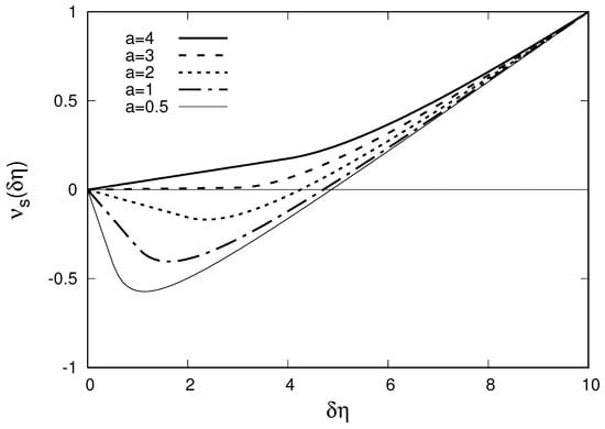
Figure 2. The same as in Figure 1, but for the observable ${\nu }_s\left(\delta \eta \right)\equiv -\frac{⟨n⟩}{4}{\nu }_{dyn}\left(\delta \eta \right)$, (7), as a function of rapidity width of the observation window, $\delta \eta$, in the toy model with soft correlation between identical charges, considered in Section 5.2.

By Formula (67), we see also that at

$$\delta \eta <a<(1-1/\sqrt{2})Y\approx 0.29Y$$

(68)

(the same condition as the condition obtained from Formula (64) for the BF), the ${\nu }_s\left(\delta \eta \right)$ is negative, ${\nu }_s\left(\delta \eta \right)<0$ (see Figure 2, plotted for $Y=10$), and cannot be interpreted as a probability.

Note that this occurs for rather wide correlation function ${\lambda }_{++}({\eta }_1-{\eta }_2)$ (58), with a compared to Y, as follows from Condition (68).

In Appendix C, we perform one more check of the obtained formulae. We analyze the limiting cases of the model with a soft correlation between identical charges, given by a function (see Formulae (57) and (58)):

$${\lambda }_{++}\left(\mathsf{\Delta }\eta \right)=\frac{2}{Y-a/2}{h}_a\left(\mathsf{\Delta }\eta \right)=\frac{1}{(2Y-a)a}\theta (a-|\mathsf{\Delta }\eta \left|\right),$$

(69)

and formulated in the present Section 5.2 for an arbitrary value of the parameter a, $0<a\le Y$, which determines the correlation length. We show that, on the one hand, for $a\to 0$, the model turns into a version with a strict correlation between identical charges considered in Section 5.1, and on the other hand, for $a=Y$, it goes to the model with the production of uncorrelated charge pairs by the source, discussed in Section 4.

We also see that the negative values of the BF $B\left(\mathsf{\Delta }\eta \right)$ at $\mathsf{\Delta }\eta <a$ and the ${\nu }_s\left(\delta \eta \right)$ at $\delta \eta <a$ already occur when we introduce the rather weak correlation between same charge particles with the value of a compared to Y, namely at $a<(1-1/\sqrt{2})Y\approx 0.29Y$, as follows from Condition (68) (see Figure 1 and Figure 2).

6. Summary

In this short note, by constructing a simple toy model, we explicitly demonstrate that the values of the ${\nu }_s\left(\delta \eta \right)$ and hence the ${\nu }_{dyn}\left(\delta \eta \right)$, for which by (7) we have

$${\nu }_s\left(\delta \eta \right)\equiv -\frac{⟨n⟩}{4}{\nu }_{dyn}\left(\delta \eta \right),$$

can be both negative and positive. Therefore, it cannot have any probabilistic interpretation, such as, for example, the probability that balancing charges occur in the same rapidity interval $\delta \eta$, which is discussed, e.g., in the paper [6] (see comments after Formula (4)).

Then, by the relation

$${\nu }_s\left(\delta \eta \right)=\frac{1}{\delta \eta }{\int }_{\delta \eta }d{\eta }_1{\int }_{\delta \eta }d{\eta }_{2}B({\eta }_1-{\eta }_2),$$

it follows that in this case the BF must also be negative at least for some values of $\mathsf{\Delta }\eta ={\eta }_1-{\eta }_2$ to ensure the negative value of the integral. We also check this explicitly by computing the BF in our toy model.

Since BF $B\left(\mathsf{\Delta }\eta \right)$ can take negative values, it also cannot have any probabilistic interpretation in the general case. In particular, the BF cannot be interpreted as the probability density for the balancing charges to occur separated by the rapidity interval $\mathsf{\Delta }\eta$, as was formulated in the paper [7].

References

- Jeon, S.; Koch, V. Charged Particle Ratio Fluctuation as a Signal for QGP. Phys. Rev. Lett. 2000, 85, 2076. [Google Scholar] [CrossRef] [PubMed] [Green Version]
- Adcox, K.; Adler, S.S.; Ajitanand, N.N.; Akiba, Y.; Alexander, J.; Aphecetche, L.; Arai, Y.; Aronson, S.H.; Averbeck, R.C.; Awes, T.; et al. [PHENIX Collaboration] Net Charge Fluctuations in Au+Au Interactions at sNN = 130 GeV. Phys. Rev. Lett. 2002, 89, 082301. [Google Scholar] [CrossRef] [PubMed] [Green Version]
- Pruneau, C.; Gavin, S.; Voloshin, S. Methods for the study of particle production fluctuations. Phys. Rev. C 2002, 66, 044904. [Google Scholar] [CrossRef] [Green Version]
- Abelev, B.I.; Aggarwal, M.M.; Ahammed, Z.; Anderson, B.D.; Arkhipkin, D.; Averichev, G.S.; Bai, Y.; Balewski, J.; Barannikova, O.; Barnby, L.S.; et al. [STAR Collaboration] Beam-Energy and System-Size Dependence of Dynamical Net Charge Fluctuations. Phys. Rev. C 2009, 79, 024906. [Google Scholar] [CrossRef] [Green Version]
- Abelev, B.; Adam, J.; Adamová, D.; Adare, A.M.; Aggarwal, M.M.; Aglieri Rinella, G.; Agocs, A.G.; Agostinelli, A.; Aguilar Salazar, S.; Ahammed, Z.; et al. [ALICE Collaboration] Net-Charge Fluctuations in Pb-Pb Collisions at sNN = 2.76 TeV. Phys. Rev. Lett. 2013, 110, 152301. [Google Scholar] [CrossRef] [PubMed] [Green Version]
- Altsybeev, I. Baselines for higher-order cumulants of net-charge distributions from balance function. arXiv 2020, arXiv:2002.11398. [Google Scholar]
- Bass, S.; Danielewicz, P.; Pratt, S. Clocking hadronization in relativistic heavy ion collisions with balance functions. Phys. Rev. Lett. 2000, 85, 2689. [Google Scholar] [CrossRef] [PubMed] [Green Version]
- Vechernin, V.; Andronov, E. Strongly Intensive Observables in the Model with String Fusion. Universe 2019, 5, 15. [Google Scholar] [CrossRef] [Green Version]
- Vechernin, V. Forward-backward correlations between multiplicities in windows separated in azimuth and rapidity. Nucl. Phys. A 2015, 939, 21–45. [Google Scholar] [CrossRef] [Green Version]
- Gorenstein, M.I.; Gazdzicki, M. Strongly intensive quantities. Phys. Rev. C 2011, 84, 014904. [Google Scholar] [CrossRef]
- Andronov, E.V. Influence of the quark-gluon string fusion mechanism on long-range rapidity correlations and fluctuations. Theor. Math. Phys. 2015, 185, 1383–1390. [Google Scholar] [CrossRef]
- Andronov, E.; Vechernin, V. Strongly intensive observable between multiplicities in two acceptance windows in a string model. Eur. Phys. J. A 2019, 55, 14. [Google Scholar] [CrossRef] [Green Version]
Publisher’s Note: MDPI stays neutral with regard to jurisdictional claims in published maps and institutional affiliations. |
© 2021 by the author. Licensee MDPI, Basel, Switzerland. This article is an open access article distributed under the terms and conditions of the Creative Commons Attribution (CC BY) license (https://creativecommons.org/licenses/by/4.0/).