On the Optimality of the LR Test for Mediation

Abstract

Testing for mediation, or indirect effects, is empirically very important in many disciplines. It has two obvious symmetries that the testing procedure should be invariant to. The ordered absolute t-statistics from two ordinary regressions are maximal invariant under the associated groups of transformations. Sobel’s (1982) Wald-type and the LR test statistic are both functions of this maximal invariant and satisfy two logical coherence requirements: (1) size coherence: rejection at level $\alpha$ implies rejection at all higher significance levels; and (2) information coherence: more (less) evidence against the null implies continued (non) rejection of the null. The LR test statistic is simply the smallest of the two absolute t-statistics, and we show that the LR test is the Uniformly Most Powerful (information and size) Coherent Invariant (UMPCI) test. In short: the LR test for mediation is simple and best.

1. Introduction

Testing for mediation is empirically extremely important in many scientific disciplines. For example, in psychology: Baron and Kenny [1], which has more than 100,000 citations; in accounting: Coletti et al. [2]; in marketing: MacKenzie et al. [3]; in sociology: Alwin and Hauser [4]; in economics: Huber [5], amongst many others. It has also generated much methodological interest because it is a non-standard problem. Despite its great popularity, Sobel’s original test has serious shortcomings, including extremely low rejection probabilities when the indirect effect is small or estimated with large variance. See MacKinnon et al. [6] for an overview of various testing procedures. The aim of mediation testing is to establish if the causal mechanism of the effect that an independent variable (X) has on a dependent variable (Y) is via a mediating variable (M). The most basic version of the model with all variables in deviation from their means is:

$$\begin{array}{cc}\hfill Y& =\beta X+{\theta }_{2}M+u,\hfill \end{array}$$

(1)

$$\begin{array}{cc}\hfill M& ={\theta }_{1}X+v,\hfill \end{array}$$

(2)

where disturbances u and v are assumed to be independent, since Y does not influence $M,$ e.g., because of the experimental set up. The causal variable X affects Y via two different pathways. The first is the direct effect of X on Y and is quantified by $\beta .$ The second is the indirect effect of X on Y via the mediating variable M. This mediation effect is quantified by ${\theta }_1{\theta }_2$ and only exists if both ${\theta }_1$ and ${\theta }_2$ are non-zero. The null hypothesis of no mediation is commonly expressed as:

$$H_0:{\theta }_1{\theta }_2=0,$$

but it is not a standard testing problem, since the null has a singular point in the origin where the two axes (${\theta }_1=0$ and ${\theta }_2=0$) cross (see Drton [7]) and the distribution of the test statistic is non-standard as a result.

The famous test by Sobel [8] is a Wald-type test that standardizes the estimator ${\widehat{\theta }}_1{\widehat{\theta }}_2$. The test can be expressed in terms of the absolute values of ordinary t-statistics $\left(|T_1|,|T_2|\right)$ in (1) and (2). This renders a test that is invariant to the parameter value $\beta$ and to the variances of u and v. This is no coincidence: all invariant testing procedures that exploit all the information in the data and the model must be based on $\left(|T_1|,|T_2|\right)$ since it is a maximal invariant as we will see below.

An obvious alternative to the Wald test is the Likelihood Ratio (LR) test, which provides an optimal test when the null and alternative are both simple. Testing for mediation, however, involves composite null and alternative hypotheses, as well as nuisance parameters. The Neyman-Pearson lemma is not applicable, and no uniformly most powerful test exists.

We show, nevertheless, that a uniformly most powerful test exists within a class of procedures that are information coherent and invariant. Information coherence is the logical requirement introduced in Section 3, that, when information against the null increases, a test should continue to reject. It differs from the common size coherence that requires the same when the size (maximum probability of a Type I error) is increased. Both these coherency requirements are very mild. The LR test is the best coherent invariant test. Establishing this result is the main contribution of this paper.

A likelihood analysis of the estimators and LR test for mediation requires a distributional assumption. We will assume a normal distribution for each observation $1\le i\le n$: ${\left(u_i,v_i\right)}^{\prime }$∼$IIN\left(0,diag\left({\sigma }_{11},{\sigma }_{22}\right)\right).$ This is convenient, but the analysis is also valid asymptotically without assuming normality of the errors, since the t-statistics used are still asymptotically normal.

The joint density of $\left(Y,M\right)$ given X can be written as:

$$f_{Y,M|X}\left(y,m|x;\lambda \right)=f_{Y|M,X}\left(y|m,x;{\lambda }_1\right)\times f_{M|X}\left(m|x;{\lambda }_2\right),$$

with ${\lambda }_1={\left(\beta ,{\theta }_2,{\sigma }_{11}\right)}^{\prime }$, ${\lambda }_2={\left({\theta }_1,{\sigma }_{22}\right)}^{\prime }$, and $\lambda ={\left({\lambda }_1^{\prime },{\lambda }_2^{\prime }\right)}^{\prime }$. The parameters ${\lambda }_1$ and ${\lambda }_2$ vary freely as a result of the triangular (recursive) structure of the model. The mediation variable is the endogenous variable in (2), but is exogenous for ${\theta }_2$ in (1). There is no feedback or causal relation from Y to M. This can easily be extended to include more regressors/covariates. This will affect the degrees of freedom in finite samples, but not the asymptotic distribution of the t-statistics. One could also use instrumental variables, but X and M appear in both equations and in the standard setup u and v are independent because of the experimental interpretation of M and, without it, parameters are not identified. The log-likelihood given n independent observations is the sum of two Gaussian log-likelihoods corresponding to (1) and (2):

$$\ell \left(\lambda \right)\propto -\frac{1}{2{\sigma }_{11}}\sum _{i=1}^n{\left(y_i-\beta x_i-{\theta }_2{m}_i\right)}^2-\frac{n}{2}log\left({\sigma }_{11}\right)-\frac{1}{2{\sigma }_{22}}\sum _{i=1}^n{\left(m_i-{\theta }_1{x}_i\right)}^2-\frac{n}{2}log\left({\sigma }_{22}\right).$$

(3)

As a consequence, the Maximum Likelihood Estimators (MLEs) for ${\theta }_1$ and ${\theta }_2$ are the usual OLS estimators for the two equations separately. The MLE for the full $\lambda$ is minimal sufficient, and its dimension is equal to the number of parameters. The model is a full exponential model (see Van Garderen [9]), and the MLE is a complete sufficient statistic. Inference on the parameters can, therefore, be based on the MLE without loss of information. Randomization in the test procedure will lead to a loss of information and power. Hence, we will not consider randomized tests or bootstrap procedures. Finally, the information matrices will be block diagonal in ${\lambda }_1$ and ${\lambda }_2$ as well as in ${\left(\beta ,{\theta }_2\right)}^{\prime }$, ${\sigma }_{11}$, ${\theta }_1,$ and ${\sigma }_{22}.$ As a result the standard t-statistics, $T_1$ and $T_2$ for ${\theta }_1$ and ${\theta }_2$ are asymptotically independent and normally distributed.

2. Symmetry and Invariance

It is clear that the problem has a number of symmetries and invariances. The null hypothesis of no mediation ${\theta }_1{\theta }_2=0$ remains true or false if we:

(i)

Interchange ${\theta }_1$ and ${\theta }_2;$

(ii)

Change the signs of ${\theta }_1$ or ${\theta }_2$;

(iii)

Change the values of the nuisance parameters ${\sigma }_{11}$, ${\sigma }_{22},$ or $\beta .$

We want a test procedure that respects these symmetry and invariance properties. This may not be straightforward because the distributions of test statistics will generally depend on nuisance parameters, even under the null. Moreover, the t-statistics have different degrees of freedom. We will first establish the maximal invariance of the two t-statistics under a group of location-scale transformations in finite samples. This covers the invariance with respect to nuisance parameters in (iii). Invariant procedures based on the minimal sufficient statistics should depend on the t-statistics only, in finite samples as well as asymptotically. By moving to the asymptotic normal distribution, we can abstract from the difference in the degrees of freedom and consider the permutation invariance in (i) and the reflection invariance in (ii).

The finite-sample distribution involves t-distributions with different degrees of freedom and is further complicated by the fact that the standard deviation of ${\widehat{\theta }}_2$, ${\sigma }_{{\widehat{\theta }}_2},$ depends on M. Even in finite samples, however, we can derive exact results that provide a strong justification for restricting attention to the t-statistics. Proposition 1, derived in Hillier et al. [10], is a particular case in point and establishes that T is a maximal invariant regardless of sample size.

Proposition 1.

The testing problem is invariant under the group $\mathbf{K}$ of transformations acting on $\left(\widehat{\beta },{\widehat{\theta }}_2,s_{11},{\widehat{\theta }}_1,s_{22}\right)$ defined by:

$$\begin{array}{cc}\hfill \left(\widehat{\beta },{\widehat{\theta }}_2,s_{11},{\widehat{\theta }}_1,s_{22}\right)& \to \left(\sqrt{a_1}\left(\widehat{\beta }+a_0\right),\sqrt{a_1/a_2}{\widehat{\theta }}_2,a_1{s}_{11},\sqrt{a_2}{\widehat{\theta }}_1,a_2{s}_{22}\right),\hfill \\ \hfill & a_0\in \mathbb{R},a_1,a_2\in {\mathbb{R}}^{+}.\hfill \end{array}$$

The induced group of transformations $\overline{\mathbf{K}}$ acting on the parameter space is defined by:

$$\left(\beta ,{\theta }_2,{\sigma }_{11},{\theta }_1,{\sigma }_{22}\right)\to \left(\sqrt{a_1}\left(\beta +a_0\right),\sqrt{a_1/a_2}{\theta }_2,a_1{\sigma }_{11},\sqrt{a_2}{\theta }_1,a_2{\sigma }_{22}\right)$$

The vector of t-statistics is a maximal invariant statistic under the group of transformations $\mathbf{K}$:

$$T={(T_1,T_2)}^{\prime }={\left({\widehat{\theta }}_1/\sqrt{\frac{1}{n-2}{s}_{22}{\left(x^{\prime }x\right)}^{-1}},{\widehat{\theta }}_2/\sqrt{\frac{1}{n-3}{s}_{11}/s_{22}}\right)}^{\prime }.$$

A parameter-space maximal invariant under the induced group $\overline{\mathbf{K}}$ is:

$$\mu ={\left({\mu }_1,{\mu }_2\right)}^{\prime }={\left({\theta }_1/\sqrt{{\sigma }_{22}{\left(x^{\prime }x\right)}^{-1}},{\theta }_2/\sqrt{\frac{{\sigma }_{11}}{{\sigma }_{22}/n}}\right)}^{\prime }.$$

The distribution of ${(T_1,T_2)}^{\prime }$ depends only on ${({\mu }_1,{\mu }_2)}^{\prime }.$

This proposition justifies restricting the attention to the two t-statistics, even in finite samples. The proof is given in Hillier et al. [10] and further establishes that $T_1$ and $T_2$ are independent. The t-statistic $T_2$ has one degree of freedom less than $T_1$, since (1) has one more variable than (2). This difference compromises the permutation symmetry but is practically unimportant, unless the number of observations is small, for instance, less than 30. Throughout the rest of the paper, we will, therefore, use the limiting normal distribution for the t-statistics. Hence, let $\mu ={\left({\mu }_1,{\mu }_2\right)}^{\prime }={\left({\theta }_1^0/{\sigma }_{{\theta }_1},{\theta }_2^0/{\sigma }_{{\theta }_2}\right)}^{\prime }$ where ${\theta }_1^0$, ${\theta }_2^0$ denote the true parameter values and ${\sigma }_{{\theta }_1}$, ${\sigma }_{{\theta }_2}$ the standard deviations of the OLS estimators, then asymptotically:$\left(T-\mu \right)\stackrel{d}{\to }N\left(0,I_2\right)$, but we continue as if this is the exact distribution and state this explicitly in:

Assumption 1.

Gaussian Shift Experiment

$$T\sim N\left(\mu ,I_2\right)$$

Turning to symmetries (i) and (ii), let ${\mathbf{G}}_1$ be the group of permutations and ${\mathbf{G}}_2$ the group of reflections or sign changes. The two groups only have the identity element in common, and the full group $\mathbf{G}={\mathbf{G}}_1\times {\mathbf{G}}_2$, generated by ${\mathbf{G}}_1$ and ${\mathbf{G}}_2$, has $2!2^2=8$ elements. The density after a sign change in $T_k$ is obtained by a corresponding sign change in ${\mu }_k$, and density for a permutation of T is also obtained by permuting $\mu$ accordingly. Hence, for any element g$\in \mathbf{G}$, we have $\mathbf{g}·T$∼$N\left(\mathbf{g}·\mu ,I_2\right)$ or $P_{\mathbf{g}\mu }\left[\mathbf{g}T\in A\right]=P_{\mu }\left[T\in A\right]$, so the distribution is invariant; see Lehmann and Romano [11].

It is clear that the absolute order statistic, denoted $({\left|T\right|}_{\left(1\right)},{\left|T\right|}_{\left(2\right)})$ with $0\le {\left|T\right|}_{\left(1\right)}\le {\left|T\right|}_{\left(2\right)}$, is invariant because its value does not change by permuting or changing signs in T. It is also maximal invariant because, for two T and $\tilde{T}$ such that $({\left|T\right|}_{\left(1\right)},{\left|T\right|}_{\left(2\right)})=\left(\right|\tilde{T}{|}_{\left(1\right)},|\tilde{T}{|}_{\left(2\right)})$, this can only occur if the two elements in $\tilde{T}$ are a permutation of the two elements in T and possible changes in signs of the elements. There must exist a transformation $\mathbf{g}={\mathbf{g}}_1·{\mathbf{g}}_2\in G_1\times G_2$ s.t. $\tilde{T}=\mathbf{g}·T.$ The same argument holds for the ordered absolute parameter $({\left|\mu \right|}_{\left(1\right)},{\left|\mu \right|}_{\left(2\right)})$ since the group of transformations is the same on parameter and sample space. We have, therefore, established the following:

Proposition 2.

The testing problem $H_0:{\mu }_1{\mu }_2=0$ is invariant under the group of transformations $\mathbf{G}={\mathbf{G}}_1\times {\mathbf{G}}_2$ acting on T and μ, given Assumption 1. The absolute order statistic $\left({\left|T\right|}_{\left(1\right)},{\left|T\right|}_{\left(2\right)}\right)$ with $0\le {\left|T\right|}_{\left(1\right)}\le {\left|T\right|}_{\left(2\right)}$ is a maximal invariant statistic, and the absolute order parameter $\left({\left|\mu \right|}_{\left(1\right)},{\left|\mu \right|}_{\left(2\right)}\right)$ with $0\le {\left|\mu \right|}_{\left(1\right)}\le {\left|\mu \right|}_{\left(2\right)}$ is a maximal invariant parameter under the group of transformations$\mathbf{G}={\mathbf{G}}_1\times {\mathbf{G}}_2.$ The distribution of $({\left|T\right|}_{\left(1\right)},{\left|T\right|}_{\left(2\right)})$ depends only on $({\left|\mu \right|}_{\left(1\right)},{\left|\mu \right|}_{\left(2\right)}).$

Note that $({\left|T\right|}_{\left(1\right)},{\left|T\right|}_{\left(2\right)})$ is a function of the complete sufficient statistics and, hence, a maximal invariant that exploits all the information in the data. A randomized test or another procedure that is not a function of $({\left|T\right|}_{\left(1\right)},{\left|T\right|}_{\left(2\right)})$ cannot do better in terms of power.

For deriving the joint distribution of this maximal invariant $({\left|T\right|}_{\left(1\right)},{\left|T\right|}_{\left(2\right)})$, first note that if scalar T∼$N\left(\mu ,1\right),$ then $\left|T\right|$ has the folded normal distribution (noncentral Chi-distribution with one degree of freedom) with density:

$$f_{\left|T\right|}(t,\mu )=\varphi (t+\mu )+\varphi (t-\mu )=\sqrt{\frac{2}{\pi }}exp(-(t^2+{\mu }^2)/2)cosh\left(\mu t\right),\mathrm{for}t\ge 0,$$

(4)

with $\varphi \left(·\right)$ the standard normal density function. Second, $\left|T_1\right|$ and $\left|T_2\right|$ are independent and, hence, by Equation (6) of Vaughan and Venables [12], we obtain after simplification:

Lemma 1.

The density of the maximal invariant stated in Proposition 2 equals:

$$\begin{array}{cc}\hfill f_{{\left|T\right|}_{\left(1\right)},{\left|T\right|}_{\left(2\right)}}(t_1,t_2,{\mu }_1,{\mu }_2)=& \frac{2}{\pi }\left\{cosh\left(t_1{\mu }_1\right)cosh\left(t_2{\mu }_2\right)+cosh\left(t_1{\mu }_2\right)cosh\left(t_2{\mu }_1\right)\right\}\hfill \\ & \times e^{-(t_1^2+t_2^2+{\mu }_1^2+{\mu }_2^2)/2},for0\le t_1\le t_2.\hfill \end{array}$$

(5)

3. Test Statistics, Critical Regions, and Coherence

The previous section established that invariant test procedures should be based on the ordered absolute t-statistic. The classic test by Sobel [8] and the LR test are both functions of $({\left|T\right|}_{\left(1\right)},{\left|T\right|}_{\left(2\right)})$. The Sobel test statistic is the square root of the Wald statistic W based on ${\widehat{\theta }}_1{\widehat{\theta }}_2$ and its standard error derived by the delta method:

$$\sqrt{W}={\left(\frac{T_1^2{T}_2^2}{T_1^2+T_2^2}\right)}^{1/2}=\frac{{\left|T\right|}_{\left(1\right)}{\left|T\right|}_{\left(2\right)}}{\sqrt{{\left|T\right|}_{\left(1\right)}^2+{\left|T\right|}_{\left(2\right)}^2}}.$$

(6)

The LR test statistic is easily obtained by maximizing the log-likelihood with and without the restriction that either ${\theta }_1$ or ${\theta }_2$ is zero and:

$$LR=min\left\{\left|T_1\right|,\left|T_2\right|\right\}={\left|T\right|}_{\left(1\right)}.$$

(7)

An equivalent LR test can also be based on the minimum of two F-statistics $f_1=T_1^2$ and $f_2=T_2^2.$

In both cases, we reject when the test statistic is larger than the two-sided critical value from a standard normal distribution. The rejection probability for both tests is monotonically increasing in ${\left|\mu \right|}_{\left(2\right)}$ under the null with ${\left|\mu \right|}_{\left(1\right)}=0$. The size, i.e., the maximum rejection probability under $H_0$, is attained when ${\left|\mu \right|}_{\left(2\right)}\to \infty .$ The largest absolute t-value will diverge in that case, and the Sobel and LR test simply reject when the smallest absolute t-value is larger than the usual critical value, $1.96$ for a $5\%$ level test.

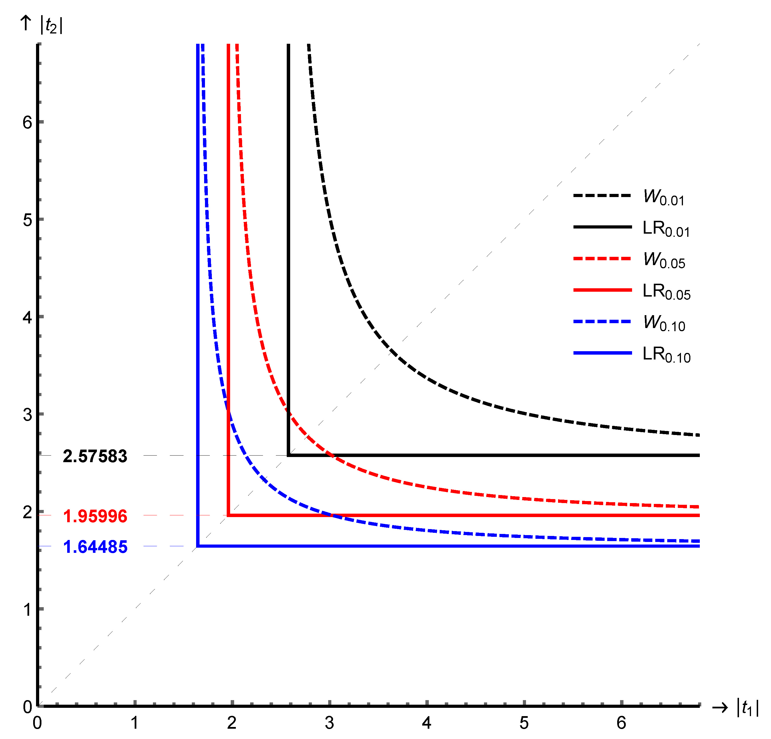
Rather than the one-dimensional test statistics, we can define tests in terms of their critical region (CR) in the sample space of dimension two. The sample space for $\left(\left|T_1\right|,\left|T_2\right|\right)$ is the quadrant ${\mathbb{R}}_{+}^2$, and the sample space for the maximal invariant $({\left|T\right|}_{\left(1\right)},{\left|T\right|}_{\left(2\right)})$ is an octant in ${\mathbb{R}}^2$: with $\mathbb{T}=\left\{({\left|T\right|}_{\left(1\right)},{\left|T\right|}_{\left(2\right)})\in {\mathbb{R}}_{+}^2\left|0\le {\left|T\right|}_{\left(1\right)}\le {\left|T\right|}_{\left(2\right)}\le \infty \right.\right\}.$ The LR critical region is:

$$C{R}_{LR}\left(\alpha \right)=\left\{\mathbb{T}\left|z_{\alpha /2}\le {\left|T\right|}_{\left(1\right)}\le {\left|T\right|}_{\left(2\right)}\le \infty \right.\right\},$$

with $z_{\alpha /2}$ the (two-sided) critical value of standard normal variate, i.e., $P\left[\left|Z\right|>z_{\alpha /2}\right]=\alpha .$

The boundary of the critical regions for the LR and Sobel test in the sample space for $\left(\left|T_1\right|,\left|T_2\right|\right)$ are given in Figure 1.

Both the LR and Wald CR have two desirable properties. First, if they reject at level $\alpha ,$ then they also reject at any other level that is larger than $\alpha .$ Second, if evidence against the null is accumulating by increasing one or both of the t-statistics, the tests will continue to reject, and, if evidence is decreasing, they will continue to accept (not reject) the null hypothesis. The first property we call size or $\alpha$ coherence, with $\alpha$ added to the usual term to distinguish it from the second property we call information coherence. We formalize these concepts next. This allows us to prove the main theorem that the LR is the most powerful CR that respects both coherence properties.

Information and Size Coherence

In general, it is desirable for testing procedures to continue to reject if the evidence against the null hypothesis is increased and to continue to accept (i.e., not reject) when evidence against the null is decreasing. Thus, if a t-statistic for a single parameter in a one-sided alternative is increasing and we reject for $t=2,$ then we should also want to reject for $t>2$ because this represents a value that is even less likely, more extreme, under the null and commonly interpreted as more evidence against the null. In multivariate settings, this is less trivial because no uniformly most powerful test exists, and the separate test statistics might be correlated. Nevertheless, in the mediation case with $H_0:{\theta }_1=0\vee {\theta }_2=0$, the two t-tests are independent, and it seems reasonable to require that one continues to reject when either $t_1$ and/or $t_2$ is increasing in absolute value, since the information against the null is strengthening, and continue to accept when either $t_1$ and/or $t_2$ is decreasing towards 0, since the information against the null is weakened. We define a class of size $\alpha$ critical regions that formalizes this requirement and show that the LR test is optimal in this class of tests that respects information coherence. Consider $CR$ and acceptance region ($AR$) for $(\left|T_1\right|,\left|T_2\right|)\in {\mathbb{R}}_{+}^2.$

Definition 1.

Information Coherence.${\mathbb{C}}_{\alpha }$ is the class of all information coherent critical regions of size α defined by the property that, with ${\delta }_1,{\delta }_2\in {\mathbb{R}}_{+}$

(i) 

for any $CR\in {\mathbb{C}}_{\alpha }$ if $(\left|T_1\right|,\left|T_2\right|)\in CR\Rightarrow \left(\left|T_1\right|+{\delta }_1,\left|T_2\right|+{\delta }_2\right)\in CR$, or, equivalently,

(ii) 

for any $AR\in {\mathbb{C}}_{\alpha }$ if $(\left|T_1\right|,\left|T_2\right|)\in AR\Rightarrow \left(\left|T_1\right|-{\delta }_1,\left|T_2\right|-{\delta }_2\right)\in AR.$

Traditional ($\alpha$) coherence is a property of a family of CRs when the size of the test varies, but information coherence considers a fixed $\alpha$ and varying values of the test statistics.

Definition 2.

Size Coherence. A family of $CR\left(\alpha \right)$ indexed by its size α is size or α coherent iff $CR\left(\alpha \right)\subseteq CR\left(\tilde{\alpha }\right)\iff$ $\alpha \le \tilde{\alpha }$.

A smaller significance level requires more extreme observations and, hence, a smaller CR. Note that the definition of $\alpha$ coherence does not require the definition of the statistics involved, but information coherence uses explicit statistics.

We show in Appendix A that a family of information coherent $CRs$ has the following properties, with $\partial CR$ the boundary of $CR$ in ${\mathbb{R}}_{+}^2$ that separates the CR from the AR, and $c{v}_1\left(t\right)$ and $c{v}_2\left(t\right)$ the critical values for $\left|T_1\right|$ and $\left|T_2\right|$, respectively, either simultaneously or conditional on the other:

Proposition 3.

Any $CR\in {\mathbb{C}}_{\alpha }$ and its boundary $\partial CR$ have the following topological and statistical properties:

(i) 

$CR$ is simply connected.

(ii) 

$\partial CR$ is a continuous plane curve.

(iii) 

$\partial CR$ is monotonically weakly decreasing.

(iv) 

$\partial CR$ can be parametrically represented globally as $\partial CR\left(\tau \right)=\left(c{v}_1\left(\tau \right),c{v}_2\left(\tau \right)\right)$ using a one-dimensional $\tau \in \mathbb{R}$, and locally as $\partial CR\left(t_1\right)=\left(t_1,c{v}_2\left(t_1\right)\right)$ if not vertical, and/or $\partial CR\left(t_2\right)=\left(t_2,c{v}_1\left(t_2\right)\right)$ if not horizontal.

(v) 

The class ${\mathbb{C}}_{\alpha }$ contains critical regions that may not be convex, but no critical regions that are strictly concave.

(vi) 

A test with $CR\in {\mathbb{C}}_{\alpha }$ can only be size correct and admissible if ${lim}_{t_1\to \infty }c{v}_2\left(t_1\right)=z_{\alpha /2}.$

Proposition 3 is instrumental in proving the optimality of the LR test and showing that the Sobel and LR tests are information and size coherent.

Proposition 4.

The Sobel (Wald) test and LR test of size α, both respect

-

information coherence: $C{R}_{\sqrt{W}}\left(\alpha \right),C{R}_{LR}\left(\alpha \right)\in {\mathbb{C}}_{\alpha }$ as well as

-

size coherence: $C{R}_{LR}\left(\alpha \right)\subset C{R}_{LR}\left(\tilde{\alpha }\right)$ and $C{R}_{\sqrt{W}}\left(\alpha \right)\subset C{R}_{\sqrt{W}}\left(\tilde{\alpha }\right)$ iff $\tilde{\alpha }>\alpha$.

This result only states that both tests share two desirable properties, but does not imply that both tests are equally good. The power of the LR is much better than Sobel’s test, which suffers from extremely low power when the mediation effect is small or is inaccurately estimated. In fact, the LR test is better than any other coherent test in ${\mathbb{C}}_{\alpha }$, which we are now able to state and prove in the main theorem of the paper.

Theorem 1.

The LR test of size α is the uniformly most powerful test in ${\mathbb{C}}_{\alpha }$.

Proof. 

The $C{R}_{LR}\left(\alpha \right)=\left\{min\left\{\left|T_1\right|,\left|T_2\right|\right\}\ge z_{a/2}\right\}$ sets the critical value for the $c{v}_1\left(t_2\right)=z_{\alpha /2}$ for all $t_2\ge t_1\ge 0$, which is the smallest value that $c{v}_1$ can take for all values of $t_2$ while still being size-correct according to (iii) and (iv) of Proposition 3. Analogously, $c{v}_2\left(t_1\right)=z_{\alpha /2}$ for all $t_1\ge t_2.$ So $C{R}_{LR}\left(\alpha \right)$ is the closure of ${\mathbb{C}}_{\alpha }$ and any member $CR\left(\alpha \right)\subseteq C{R}_{LR}\left(\alpha \right)$. Hence, $P\left[C{R}_{LR}\left(\alpha \right)\mid H_a\right]$ is larger than for any other $CR\left(\alpha \right)\in {\mathbb{C}}_{\alpha }$ that is not equal to $C{R}_{LR}\left(\alpha \right)$ a.s. This holds uniformly for all values of $\mu$ under $H_0.$ □

This optimality property of the LR test is derived under coherence requirements that are very weak: it seems more than reasonable to require that any test continues to reject if more extreme outcomes are observed or if the level of the test is increased.

4. Discussion and Conclusions

This paper has exploited the symmetry present in the mediation testing hypothesis $H_0:{\theta }_1{\theta }_2=0$ and used invariance arguments to reduce the sample space to an eighth of ${\mathbb{R}}^2$. We have developed a coherence framework to formulate and analyze the requirement that increasing or decreasing information against the null leads to coherent decisions. We call tests or CRs with this property information coherent, which is distinct from the more standard (size) coherent property that tests may possess. The Sobel test is both information and size coherent, but has very poor null rejection and power properties.

The LR test is much better than the Sobel test, and this paper shows the LR test to be the best possible of all tests that satisfy the basic coherence requirements. The optimality lends support to Perlman and Wu [13] on their preference for the LR test.

Nevertheless, the LR test has some serious shortcomings, like the Sobel test, when detecting deviations from $H_0$. In particular, when both ${\theta }_1$ and ${\theta }_2$ are close to 0, or are estimated inaccurately, it is extremely conservative and the power deteriorates and goes to ${\alpha }^2$ when $\mu \to {(0,0)}^{\prime }$.

The bootstrap does not provide an answer because of the (strong) dependency on the nuisance parameter. Of course, it may provide small-sample corrections and avoid asymptotic approximations and strong distributional assumptions. However, bootstrap versions of the LR and Sobel test still lack power and are neither size nor information coherent.

Van Garderen and Van Giersbergen [14] show there is an opportunity to gain power without violating the size condition by adding a small area near the diagonal where the opportunity to detect deviations from $H_0$ are best. It is uniformly more powerful than the LR test, but is not in ${\mathbb{C}}_{\alpha }$ since the boundary $\partial CR$ is monotonically increasing and, hence, violating property (iii) of Proposition 3. Therefore, the LR test remains the optimal coherent choice for mediation testing. It is simple and best.