A Combined Model Based on EOBL-CSSA-LSSVM for Power Load Forecasting

Abstract

Inaccurate electricity load forecasting can lead to the power sector gaining asymmetric information in the supply and demand relationship. This asymmetric information can lead to incorrect production or generation plans for the power sector. In order to improve the accuracy of load forecasting, a combined power load forecasting model based on machine learning algorithms, swarm intelligence optimization algorithms, and data pre-processing is proposed. Firstly, the original signal is pre-processed by the VMD–singular spectrum analysis data pre-processing method. Secondly, the noise-reduced signals are predicted using the Elman prediction model optimized by the sparrow search algorithm, the ELM prediction model optimized by the chaotic adaptive whale algorithm (CAWOA-ELM), and the LSSVM prediction model optimized by the chaotic sparrow search algorithm based on elite opposition-based learning (EOBL-CSSA-LSSVM) for electricity load data, respectively. Finally, the weighting coefficients of the three prediction models are calculated using the simulated annealing algorithm and weighted to obtain the prediction results. Comparative simulation experiments show that the VMD–singular spectrum analysis method and two improved intelligent optimization algorithms proposed in this paper can effectively improve the prediction accuracy. Additionally, the combined forecasting model proposed in this paper has extremely high forecasting accuracy, which can help the power sector to develop a reasonable production plan and power generation plans.

1. Introduction

With the improvement in economic and social development, high-quality electric energy supply provides an important guarantee for the efficient and stable development of the whole country. The accuracy of electricity load forecasting is directly related to the economic efficiency and reliability of each energy supply sector. Many important operational decisions such as generation plans, fuel procurement plans, maintenance plans, and energy trading plans are based on electricity load forecasting [1,2,3,4].

The intrinsic properties of the electrical load make it fundamentally different from other commodities. This is due to the non-storable nature of the electricity load, which is also influenced by the dynamic balance between supply and demand and the reliability of the intelligent transmission network [5]. Accurate power load forecasting can effectively optimize the allocation of resources in intelligent distribution networks and power systems. For the supply sector of the power system, accurate load forecasting enables rational control of the capacity of generating units and rational dispatch of generating capacity, thus reducing energy wastage and costs. For the management of the power system, mastering the changes in the power load at any given moment allows them to control the power market information in advance and thus obtain higher economic benefits. In practice, the power sector often does not have access to symmetrical information. This is because inaccurate load forecasts provide the wrong information to the electricity sector, resulting in an asymmetry between the sector and the electricity consumers. The use of asymmetrical load information in production planning not only results in economic losses but also in wasted resources.

In summary, the power sector must ensure a dynamic balance between power demand and supply, while minimizing the waste of resources and economic losses [6]. Therefore, accurate electricity load forecasting is key to achieving this target.

For the above reasons, a novel combinatorial model for electricity load forecasting is proposed by this paper. The model combines a data pre-processing method (VMD–singular spectrum analysis noise reduction method), two novel combinatorial intelligent optimization algorithms (the CAWOA and EOBL-CSSA algorithm), and three independent and efficient forecasting models (ELMAN neural network, LSSVM model, ELM neural network). Firstly, the original signal is pre-processed by the VMD–singular spectrum analysis data pre-processing method. Secondly, the noise-reduced signals are predicted using the Elman prediction model optimized by the SSA algorithm, the ELM prediction model optimized by the CAWOA-ELM algorithm, and the LSSVM prediction model optimized by the EOBL-CSSA-LSSVM algorithm for electricity load data, respectively. Finally, the weighting coefficients of the three prediction models are calculated using the simulated annealing (SA) algorithm and weighted to obtain the prediction results.

2. Literature Review

Due to the rapid development of smart distribution networks, new grid planning and strategy formulations need the support of high-precision power load forecasting. Many researchers have made unremitting efforts to improve the accuracy of power load forecasting in the environment of smart distribution networks. The different forecasting principles can be divided into traditional forecasting methods based on statistics [7,8] and intelligent forecasting methods based on machine learning algorithms [9,10]. Traditional methods of forecasting electrical loads have the advantage of low computational effort and high prediction accuracy for simple linear cases. However, such methods are not sufficient to deal with complex nonlinear load time series and are difficult to meet the needs of modern forecasting. With the development of artificial intelligence (AI) technology [11,12,13], machine learning is widely used in the field of power load forecasting due to its powerful non-linear processing capability [14].

The powerful adaptive and learning capabilities of machine learning algorithms are well suited for processing non-linear time series. However, different machine learning algorithms have their own limitations, which limit their further development. Currently, swarm intelligence optimization algorithms are widely used in neural networks, machine learning, and other intelligent algorithms for structural optimization [15]. Common swarm intelligence optimization algorithms include: ant colony optimization algorithms (ACO) [16,17] and particle swarm optimization algorithms (PSO) [18,19]. In addition, such novel swarm intelligence optimization algorithms as the whale optimization algorithm (WOA) [15,20] and sparrow search algorithm (SSA) [21] also show amazing potential in processing structure optimization.

Paper [22] has shown that using raw data directly for prediction would significantly confound the results. In order to minimize the forecast error of electrical loads, scholars have carried out many studies on combined forecasting models based on data pre-processing and electrical load forecasting models. Typically, these scholars use wavelet transform (WT) [23], empirical modal decomposition (EMD) [24], variational modal decomposition (VMD) [25], and singular spectrum analysis [26] for noise reduction.

Electricity load is a complex time series with non-linear, highly random fluctuations and time-varying characteristics. The modern requirement for accurate forecasting is difficult to achieve due to the shortcomings of a single forecasting method. Therefore, the idea of combined forecasting is proposed to compensate for the shortcomings of single forecasting methods to improve the overall forecasting accuracy of the model [27].

Jinliang Zhang and his colleagues [28] proposed a hybrid forecasting model based on improved empirical modal decomposition (IEMD), autoregressive integrated moving average (ARIMA), and wavelet neural network (WNN) based on fruit fly optimization algorithm (FOA) optimization. Jinliang Zhang used the FOA algorithm to optimize the network parameters in the WNN algorithm. This approach can effectively improve the shortcomings of the WNN algorithm in terms of optimization capability. The optimized model is also combined with traditional prediction methods to improve the overall prediction accuracy. Simulation experiments demonstrate the effectiveness of this approach.

Heng Shi and his colleagues [29] proposed a method for household load prediction using deep learning and a new deep recurrent neural network based on clustering. The machine learning algorithm batches the load into the input pool to avoid overfitting. Simulation experiments also demonstrate that the model has a higher prediction accuracy than traditional prediction models.

Kun Xie and his colleagues [30] constructed a hybrid prediction model by optimizing the Elman neural network (ENN) with the PSO algorithm. The PSO algorithm was used to search for the optimal learning rate of the ENN to improve the prediction accuracy of the prediction model. Kun XI also analyzed the effect of neural network parameters on the performance of the network in detail and demonstrated that the optimization of network parameters can effectively improve the performance of the model. Finally, the effectiveness of the method was verified through simulation comparison experiments with the generalized regression neural network (GRNN) and traditional back propagation neural network (BPNN).

Zhihao Shang and his colleagues [31] used the LSSVM, ELM, and GRNN models to construct a combined prediction model. The weight coefficients of the three models were calculated using the WOA algorithm. The model was compared with the traditional BP and ARIMA models by real data. The experimental results verify that the model has excellent prediction accuracy. This is also good evidence that the use of intelligent algorithms to optimize the weighting coefficients of different models can effectively improve the prediction accuracy of the models.

Lizhen Wu and his colleagues [32] proposed a GRU-CNN neural network electricity load forecasting model based on gated recurrent units (GRU) and convolutional neural networks (CNN). Lizhen Wu used the GRU module to specifically process the feature vectors of time series data and the CNN module to process other high-dimensional data feature vectors. The effective combination of the two modules was used to improve the model prediction accuracy. Finally, the prediction performance of the model was verified by comparison experiments with BPNN, GRU, and CNN models.

Zuoxun Wang and his colleagues [33] optimized the ELM neural network with the SSA algorithm improved by firefly perturbation and chaos strategies to construct an electricity load forecasting model. The powerful optimization-seeking capability of the FA-CSSA-ELM algorithm was exploited to optimize two parameters in the ELM algorithm. Finally, a comparison experiment with other competing models was used to verify that the model can improve the prediction accuracy well.

Hairui Zhang and his colleagues [34] proposed a combined prediction model combining VMD, the Jordan neural network, the echo state network and the LSSVM model in order to overcome the shortcomings of the single prediction model. The PSO algorithm was used to optimize the relevant parameters of the neural network. This combined prediction model can make full use of the advantages of different models. Finally, the weight coefficients of the different models were calculated by the SA algorithm to obtain the final prediction results. The simulation experiments of power load forecasting also demonstrated that this model can improve the prediction accuracy of the forecasting model.

In summary, we found that the prediction performance of the combined prediction model is better than that of the single model. Additionally, we believe that there is still a huge potential for improvement in the selection and improvement of intelligent algorithms and data pre-processing for power load forecasting models, even though several of the above forecasting models have high forecasting accuracy and performance.

3. Materials and Methods

This chapter introduces VMD, singular spectrum analysis, noise reduction methods based on VMD–singular spectrum analysis, Elman neural network model, ELM neural network model, LSSVM model, WOA algorithm, CAWOA algorithm, SSA algorithm, EOBL-CSSA-LSSVM algorithm, and SA algorithm.

3.1. Variational Mode Decomposition

VMD is an adaptive solver and a completely non-recursive method for modal variation and signal processing. VMD can overcome the problems of endpoint effects and modal component confounding that exist in EMD methods. It has been demonstrated in the literature that VMD has a good decomposition effect in dealing with non-linear, non-stationary, and highly complex time series. Additionally, the specific algorithm derivation is shown in the paper [35].

3.2. Singular Spectrum Analysis

Singular spectrum analysis was first applied to oceanographic research in 1978 [36]. Nowadays, singular spectrum analysis is a common method for studying non-linear time series. The basic idea of singular spectrum analysis is to calculate its corresponding Hankel trajectory matrix H from a one-dimensional time series $\left\{h_i,i=1,\dots ,N\right\}$, as shown in Equation (1).

$$H=\left[\begin{array}{cccc}{h}_1& h_2& \cdots & h_{\mathrm{k}}\\ h_2& h_3& \cdots & h_{K+1}\\ ⋮& ⋮& \ddots & ⋮\\ h_L& h_{L+1}& \cdots & h_N\end{array}\right],$$

(1)

where H is the trajectory matrix; L is the sliding window parameter and 1 < L < N; K is defined as N − L + 1; and the eigenvalues and eigenvectors of their corresponding eigenvectors are combined to reconstruct the new time series.

3.3. VMD–Specular Spectral Analysis Noise Reduction Method

In this paper, a noise reduction approach combining VMD and singular spectrum analysis is proposed. First, the original data are adaptively decomposed and reconstructed by introducing kurtosis calculation to make the variational mode decomposition. This ensures that the reconstructed signal is close to the original signal while removing the high-frequency noise present in it. Then, the reconstructed data are second filtered by an adaptive singular spectrum analysis filter to remove the relatively low-frequency residual noise. Additionally, the kurtosis value $K\left(x\right)$ is calculated as shown in Equation (2).

$$K\left(x\right)=\frac{E\left[{\left(x-\eta \right)}^4\right]}{{\left(E\left[{\left(x-\eta \right)}^2\right]\right)}^2},$$

(2)

where E is the expectation and $\eta$ is the mean value of the series x. The calculated kurtosis value $K\left(x\right)$ is then compared with the kurtosis threshold set in this paper to select the IMF components that need to be reconstructed. Finally, the signal to be reconstructed is noise-reduced by singular spectrum analysis.

The detailed steps of the VMD–singular spectrum analysis of noise reduction method can be summarized as follows:

• Define the relevant parameters in VMD: the number of modes K and the penalty factor $\partial$;
• Input time series $f\left(t\right)$. The time series $f\left(t\right)$ is decomposed into K components of IMF by using VMD, and the decomposed components are denoted as $F=\left\{u_1,\dots ,u_k,\dots u_K\right\}$;
• The kurtosis values of the K components of IMF obtained from the VMD decomposition are calculated according to Equation (2) and noted as $Ku=\left\{K{u}_1,\dots ,K{u}_k,\dots K{u}_K\right\}$;
• Calculate the kurtosis value for each IMF component and search for IMF components greater than the kurtosis threshold;
• The IMF components obtained in step four are linearly reconstructed to obtain the VMD noise-reduced time series $f{\left(t\right)}^{\prime }$;
• For the VMD processed signal $f{\left(t\right)}^{\prime }$, choose a suitable window length parameter L to lag-arrange the original time series to construct the Hankel matrix $H_{L\times K}$;
• Singular spectrum analysis method is used to denoise Hankel matrix $H_{L\times K}$, and $H=U{\displaystyle \sum V^T}$ is obtained. U and V represent the associated left and right singular spectral vectors, respectively. Firstly, the covariance matrix $S=H{H}^T$ of the Hankel matrix H is calculated, and then the covariance matrix S is decomposed into eigenvalues to obtain ${\lambda }_1\ge {\lambda }_2\ge \dots \ge {\lambda }_L\ge 0$ and the corresponding eigenvector $U_1,U_2,\dots ,U_L$. At this point, $U=\left[U_1,U_2,\dots ,U_L\right]$ and $\sqrt{{\lambda }_1}\ge \sqrt{{\lambda }_2}\ge \dots \ge \sqrt{{\lambda }_L}\ge 0$ are singular spectra of the original sequence, which can be expressed as $H={\displaystyle \sum _{m=1}^L\sqrt{{\lambda }_m}}{U}_m{V}_m^T,V_m=\raisebox{1ex}{$H^T{U}_m$}\!\left/ \!\raisebox{-1ex}{$\sqrt{{\lambda }_m}$}\right.,m=1,\dots ,L$, where ${\lambda }_i$ is the corresponding eigenvector and $U_i$ is a time-empirical orthogonal function that can reflect the evolutionary pattern of the time series;
• Divide the L components of the trajectory matrix H into C disjoint subsets representing the different trend components;
• Reconstruct the time series. Calculate the projection $a_i^m$ of the hysteresis matrix $H_i$ onto $U_m$, $a_i^m=H_i{U}_m={\displaystyle \sum _{j=1}^L{H}_{i+j}}{U}_m,0\le i\le N-L$, where $a_i^m$ reflects the weight of $H_i$ at the time of the original series $h_{i+1},\dots ,h_{i+L}$, and N is the length of the time series. Finally, the time series is reconstructed by means of the time-empirical orthogonal function $U_i$ and the weights $a_i^m$. The specific reconstruction process can be defined as Equation (3):

  $$h_i^k=\left\{\begin{array}{c}\frac{1}{i}{\displaystyle \sum _{j=1}^i{a}_{i-j}^k{U}_{k,j},1\le i\le L-1}\\ \frac{1}{L}{\displaystyle \sum _{j=1}^L{a}_{i-j}^k{U}_{k,j},L\le i\le N-L+1}\\ \frac{1}{N-i+1}{\displaystyle \sum _{j=i-N+L}^L{a}_{i-j}^k{E}_{k,j},N-L+2\le i\le N}\end{array}\right.$$

  (3)

3.4. Elman Neural Network Model

The Elman neural network with great computational power. Each layer of the Elman neural network is independent of each other, which is why it is widely used in the field of power load forecasting [37].

Additionally, the non-linear state space expression of the Elman network can be defined as:

$$y\left(k\right)=g\left({\omega }^{3}x\left(k\right)\right),$$

(4)

$$x\left(k\right)=f\left({\omega }^1{x}_c\left(k\right)+{\omega }^2\left(u\left(k-1\right)\right)\right),$$

(5)

$$x_c\left(k\right)=x\left(k-1\right),$$

(6)

where y is the output vector; x is the unit vector; u is the input vector; $x_c$ is the state vector; ${\omega }^3$ is the weight of the output layer and the intermediate layer; ${\omega }^2$ is the weight of the input and intermediate layers; ${\omega }^1$ is the weight of the take-up layer and the intermediate layer; $g$ and $f$ is the transfer function.

3.5. Extreme Learning Machine Neural Network

Elman is a neural network with powerful generalization capabilities. However, the initial weights and thresholds of ELM are randomly assigned [38,39].

Suppose there are Q learning samples, $\left\{\left(x_l,y_l\right)\right\}{Q}_l=1$ and $x_l\in R^{\pi },y_l\in R^{\psi }$. Assume that the number of hidden layer neurons is M. The standard form is shown in Equation (7):

$${\displaystyle {\sum }_{j=1}^M{a}_j\left({\omega }_j{x}_l+b_j\right)}=f_M\left(x\right)$$

(7)

According to the zero-error approximation principle, the existence of $b_j$, $a_j$, ${\omega }_j$ reduces the normalized form to Equation (8).

$$Ha=Y,$$

(8)

where H is the output matrix, Y is the desired output matrix, and a is the output weight matrix found using the solved least squares method. Finally, the solution is continued using $a^{\prime }=H^{+}Y$. The specific mathematical model is shown in paper [38].

3.6. Least Square Support Vector Machine

LSSVM can convert complex quadratic programming problems into linear systems of equations problems and improve the speed of problem solving by replacing inequality constraints with equation constraints in SVM optimization problems [40,41].

Let the input and output of the n training samples be $\left(x_1,y_1\right),\left(x_2,y_2\right),\dots ,\left(x_i,y_i\right),i=1,2,\dots ,n$, where $x_i$ is the input vector and $y_i$ is the output vector. The optimal decision function is constructed in the high-dimensional feature space using a non-linear mapping function, as shown in Equation (9):

$$f\left(x\right)={\omega }^T\phi \left(x\right)+b,$$

(9)

where ${\omega }^T$ is the weight vector and b is a constant. The optimization objective can be expressed as Equation (10):

$$\min \frac{1}{2}‖\omega ‖+\frac{1}{2}\lambda {\displaystyle \sum _{i=1}^n{\xi }_i^2}$$

(10)

The constraint can be expressed as Equation (11):

$$y_i={\omega }^T\phi \left(x_i\right)+b+\xi ,i=1,2,\dots ,n$$

(11)

where $\lambda$ is the penalty factor and $\xi$ is the relaxation factor. Because the LSSVM can transform a quadratic programming problem into a problem of solving the above system of linear equations, the prediction model can be summarized as Equation (12).

$$y_i=b+{\displaystyle \sum _{i=1}^n{a}_i}k\left(x,x_i\right)$$

(12)

The specific mathematical derivation is shown in paper [40].

3.7. Sparrow Search Algorithm

The sparrow search algorithm is a swarm intelligence optimization algorithm proposed by Xue in 2020 [21]. The algorithm is mainly based on the foraging and anti-predation behavior of sparrows. The SSA has high search accuracy, fast convergence, high stability, and robustness compared to other population intelligence optimization algorithms. Additionally, the SSA has been successfully applied in the field of path planning [42] and structural optimization of micro-grids [43].

Sparrows in the SSA algorithm are classified as discoverers, joiners, and vigilantes. The discoverer is responsible for finding food for the entire population and providing foraging directions for the joiners, so the discoverer’s foraging search is larger than that of the joiners. During each iteration, the discoverer iterates according to Equation (13):

$$x_{id}^{t+1}=\left\{\begin{array}{c}{x}_{id}^t\cdot \exp \left(\frac{-i}{\partial \cdot T}\right),R_2<ST\\ x_{id}^t+Q\cdot L,R_2\ge ST\end{array}\right.,$$

(13)

where $t$ denotes the current number of iterations, $T$ denotes the maximum number of iterations, $\partial$ is a random number between $\left[0,1\right]$, $Q$ is a random number subject to a normal distribution, $L$ is a matrix of $1\times d$ whose elements are all 1, $R_2$ denotes a guard value, ranging from $\left[0,1\right]$, and $ST$ is a safe value, ranging from $\left[\frac{1}{2},1\right]$.

During the foraging process, some joiners will always monitor the finder, and when the finder finds better food, the joiner will compete with it. If successful, it will immediately obtain that finder’s food, otherwise the joiner will update its position according to Equation (14).

$$x_{id}^{t+1}=\left\{\begin{array}{c}{x}_{id}^t\cdot \exp \left(\frac{x{w}_d^t-x_{id}^t}{i^2}\right),i>\frac{n}{2}\\ x{b}_d^{t+1}+\frac{1}{D}{\displaystyle \sum _{d=1}^D\left(rand\left\{-1,1\right\}\cdot \left|x_{id}^t-x{b}_d^{t+1}\right|\right),i\le \frac{n}{2}}\end{array}\right.,$$

(14)

where $x{w}_d^t$ denotes the worst position in dimension $d$ of the $t$-th iteration and $x{b}_d^{t+1}$ denotes the best position. When $i>\frac{n}{2}$, it means that the population is short of food and needs to go elsewhere to forage. When $i\le \frac{n}{2}$, it means that the tracker is predating near the optimal position $xb$.

The number of sparrows aware of danger in a sparrow population is 10–20% of the total, and the location of these sparrows is randomly generated and continuously updated according to Equation (15) for the location of the vigilantes.

$$x_{id}^{t+1}=\left\{\begin{array}{c}x{b}^t+\beta \left(x_{id}^t-x{b}_d^t\right),f_i\ne f_g\\ x_{id}^t+K\left(\frac{x_{id}^t-x{w}_d^t}{\left|f_i-f_w\right|+\mu }\right),f_i=f_g\end{array}\right.,$$

(15)

where $\beta$ is the step control parameter, a normally distributed random number with a mean of 0 and a variance of 1; $K$ is a random number between $\left[-1,1\right]$; $\mu$ is a very small number, just in case the denominator is 0; $f_i$ is the current fitness; $f_g$ is the best fitness; and $f_w$ is the worst fitness.

3.8. The EOBL–CSSA Algorithm

In this paper, the chaotic mapping strategy and the elite opposition-based learning strategy are used to optimize the SSA algorithm. Firstly, the initial population is initialized by Tent chaotic mapping to improve the quality of the initial solution and enhance the global search capability of the algorithm. An elite back-learning mechanism is then introduced on top of the chaotic sparrow algorithm to extend the global search capability of the algorithm. Before extending the neighborhood of the current best individual, reverse learning is performed on it to generate a reverse search population within its search boundary, guiding the algorithm to approach the solution space containing the global optimum, thus improving the algorithm’s balancing and exploration capabilities as well as its ability to jump out of local extremes.

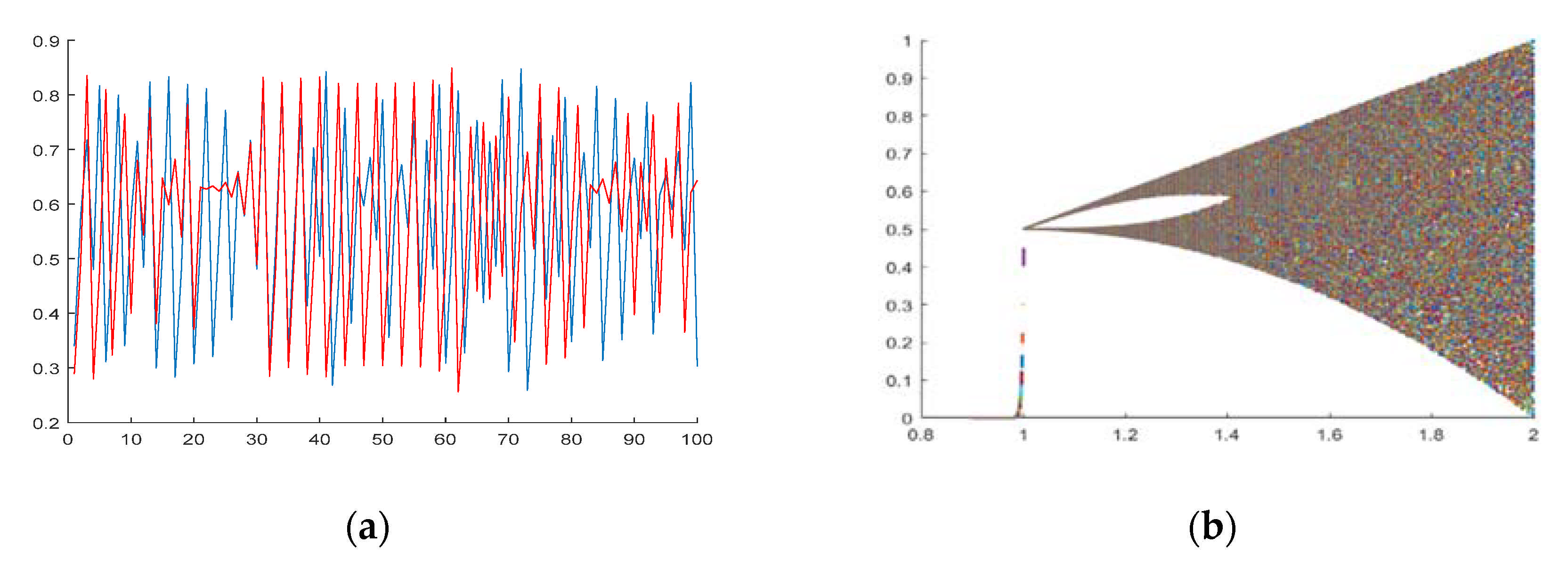
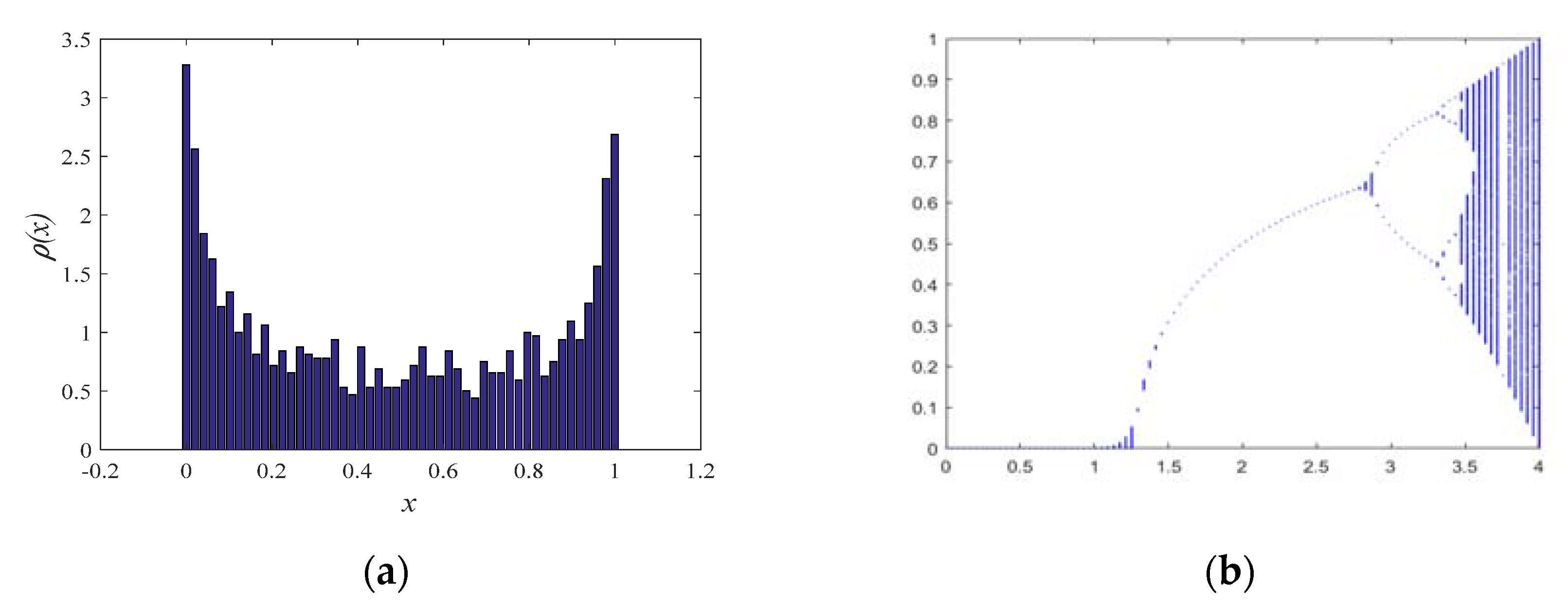
3.8.1. Tent Chaotic Mapping Strategy

The random and ergodic nature of chaos can effectively maintain the diversity of the population, helping the algorithm to jump out of the local optimum and improving the global search capability of the algorithm. It has been documented that the algorithm’s ability to find an optimum is influenced by the ergodicity of the chaotic mapping [44]. The more uniform the chaotic mapping, the faster the convergence of the algorithm. As shown in Figure 1, we can observe that the Tent chaotic mapping is well distributed and has even better traversal performance.

Suppose that in a space of dimension D, where $x=\left\{x_n,n=1,2,\dots ,D\right\}$. Additionally, the Tent chaos mapping can be expressed as Equation (16):

$$x_{n+1}=\left\{\begin{array}{c}2x_n,0\le x_n<0.5\\ 2\left(1-x_n\right),0.5\le x_n\le 1\end{array}\right.,$$

(16)

3.8.2. Elite Opposition-Based Learning Strategies

Paper [45] introduces the concept of backward learning for the first time. This method generates a reverse solution individual of the current individual in the fetching region and will select the better of the two into the next generation. It is further shown that the reverse solution has a probability of being closer to the global optimum than the current population by about 50%. The elite inverse strategy has been used in group intelligence optimization algorithms such as PSO [46], Harris Hawk Optimization (HHO) [47] and the Dragonfly Algorithm (DA) [48].

In this paper, the global search capability of the algorithm is extended by introducing an elite opposition-based learning mechanism. The strategy takes the top 10% of individuals in terms of sparrow fitness as the elite solution, while obtaining the dynamic boundaries of the elite sparrows. Before neighborhood expansion is performed on the current best sparrow individual, backward learning is performed on it to generate a reverse search population within its search boundary, guiding the algorithm to approach the solution space containing the global optimum. The sparrow position is updated by comparing the sparrow adaptation values before and after the update. If the comparison result is better, the previous sparrow is replaced. In summary, the elite opposition-based learning strategy can be a good way to improve the algorithm’s balance and exploration capabilities, thus helping the algorithm to jump out of local extremes. The elite opposition-based learning strategy can be illustrated by the following three definitions:

Theorem 1.

Reverse solution [49]: Let there exist a real number$x$on the interval$\left[a,b\right]$. Then, the reverse solution of$x$is defined as$x^{\prime }=a+b-x$. Suppose there exists a certain N-dimensional point$p=\left(x_1,\dots ,x_i,\dots ,x_N\right)$on an R-domain and$x_i\in \left[a_i,b_i\right]$. Then, define$p^{\prime }=\left(x_1^{\prime },\dots ,x_i^{\prime },\dots ,x_N^{\prime }\right)$to be the inverse of p, where$x_i^{\prime }=k\left(a_i+b_i\right)-x_i$; k is a generalized coefficient and is a uniform random number belonging within $\left[0,1\right]$.

Theorem 2.

Optimization based on reverse solutions [49]: Let the problem to be optimized be the minimum problem and the fitness function be set to $f$. If there exists some feasible solution$x$, then its reverse feasible solution is$x^{\prime }$. If$f\left(x^{\prime }\right)<f\left(x\right)$holds, then replace$x$with$x^{\prime }$.

Theorem 3.

Elite Reverse Solution [49]: Let$x_{best}^{\prime }=\left(x_1^{\prime },\dots ,x_i^{\prime },\dots x_N^{\prime }\right)$be the reverse solution of the current group of elite individuals$x_{best}=\left(x_1,\dots ,x_i,\dots x_N\right)$in some N-dimensional space, where$x_i^{\prime }=k\left(a_i+b_i\right)-x_i$;$x_i\in \left[a_i,b_i\right]$; k is a generalized coefficient and is a uniform random number belonging to the interior of$\left[0,1\right]$.

The flow of the chaotic sparrow search algorithm based on the elite opposition-based learning strategy can be summarized as follows:

• Initialize the population and the number of iterations using the Tent chaos mapping formula $x_{n+1}=\left\{\begin{array}{c}2x_n,0\le x_n<0.5\\ 2\left(1-x_n\right),0.5\le x_n\le 1\end{array}\right.$. Initialize the initial ratio of predators and joiners;
• Calculate fitness values and ranking based on the results;
• Update predator location based on $x_{id}^{t+1}=\left\{\begin{array}{c}{x}_{id}^t\cdot \exp \left(\frac{-i}{\partial \cdot T}\right),R_2<ST\\ x_{id}^t+Q\cdot L,R_2\ge ST\end{array}\right.$;
• Update joiner location based on $x_{id}^{t+1}=\left\{\begin{array}{c}{x}_{id}^t\cdot \exp \left(\frac{x{w}_d^t-x_{id}^t}{i^2}\right),i>\frac{n}{2}\\ x{b}_d^{t+1}+\frac{1}{D}{\displaystyle \sum _{d=1}^D\left(rand\left\{-1,1\right\}\cdot \left|x_{id}^t-x{b}_d^{t+1}\right|\right),i\le \frac{n}{2}}\end{array}\right.$;
• Update guard positions according to $x_{id}^{t+1}=\left\{\begin{array}{c}x{b}^t+\beta \left(x_{id}^t-x{b}_d^t\right),f_i\ne f_g\\ x_{id}^t+K\left(\frac{x_{id}^t-x{w}_d^t}{\left|f_i-f_w\right|+\mu }\right),f_i=f_g\end{array}\right.$;
• Calculate fitness values and update sparrow positions;
• Find the reverse solution of all current solutions according to the defining formula $x^{\prime }=a+b-x$ for the reverse solution;
• Those individuals whose fitness value of the original solution is greater than the fitness value of the reverse solution are selected according to the elite selection formula $f\left(x^{\prime }\right)<f\left(x\right)$ and form an elite group;
• On the new search space constructed by the elite population, the reverse solution is then found for individuals whose original solution fitness value is less than the reverse solution fitness value according to equation $x_i^{\prime }=k\left(a_i+b_i\right)-x_i$. If the algorithm converges to the global optimal solution, the search interval formed by the elite population must converge to the region where the optimal solution is located. This makes full use of the effective information of the elite population to generate the inverse solution on the dynamically defined interval formed by the elite population, guiding the search closer to the optimal solution;
• Calculate the fitness value and update the sparrow individuals and locations. Compare the sparrow individuals and locations before and after the update and compare the results with each other to see if the results are better. If the result is better, replace the previous sparrow;
• Determine whether the stop condition is met. If the condition is met, exit and output the result. Otherwise, repeat steps 2–10.

3.9. Whale Optimization Algorithm

The whale optimization algorithm is a new nature-inspired optimization algorithm proposed by Mirjalili in 2016 [20]. The WOA simulates the social behavior of humpback whales, using random or optimal search agents to model the special hunting behavior of humpback whales, and introduces a bubble attack strategy based on this. The WOA converges quickly around the optimal value and has good global optimization capability. Paper [20] systematically illustrates the mathematical model of the whale optimization algorithm.

However, the WOA has the disadvantages of uneven initial population distribution, low convergence accuracy, and insufficient global optimization capability when solving complex problems. Therefore, this paper proposes a chaotic adaptive whale algorithm on this basis.

3.10. Chaotic Adaptive Whale Optimization Algorithm

The population is initialized by the chaotic properties of the Sine chaos mapping to ensure a uniform distribution of this whale in the solution space. In addition, studies have shown that larger thresholds facilitate global exploration and smaller thresholds enhance local exploitation. Therefore, this paper introduces adaptive inertia weights to improve the convergence accuracy and global optimization capability of the algorithm. The algorithm is made to have larger inertia weights in the early iterations and smaller inertia weights in the later iterations.

3.10.1. Sine Chaotic Mapping Strategy

The mathematical model of Sine chaotic self-mapping is defined as Equation (17):

$$X_{n+1}=\frac{a}{4}\sin \left(\pi X_n\right)$$

(17)

Additionally, when $a\in \left[0,4\right]$, the algorithm is in a chaotic state. This ensures that the whales are evenly distributed in the solution space after a certain number of iterations. The Sine chaos mapping distribution is shown in Figure 2.

3.10.2. Adaptive Inertia Weights

The adaptive inertia weight is introduced to balance the global exploration capability and local exploitation capability of the algorithm. This can be a good way to improve the optimization capability of the algorithm. The mathematical model of adaptive inertia weight $\omega$ is defined as Equation (18):

$$\omega =\frac{1}{5}+\frac{1}{0.4-\exp {\left(\raisebox{1ex}{$f_{fit}\left(x\right)$}\!\left/ \!\raisebox{-1ex}{$s$}\right.\right)}^r}$$

(18)

where $f_{fit}\left(x\right)$ is the fitness value of whale $x$, r is the current number of iterations, and s is the best adaptation value for the whale population in the first iteration of the calculation. Using the dynamic nonlinearities of $\omega$ to obtain the new whale position, the optimized formula can be expressed as Equations (19) and (22):

$$X\left(t+1\right)=\omega \cdot X_d(t)-A\cdot \left|C{X}_d(t)-X\left(t\right)\right|$$

(19)

$$X\left(t+1\right)=\omega \cdot X_d\left(t\right)+\left(\left|X_d\left(t\right)-X\left(t\right)\right|\right)\cdot e^{bh}\cdot \cos \left(2\pi h\right)$$

(20)

$$X\left(t+1\right)=\left\{\begin{array}{c}\omega \cdot X_d(t)-A\cdot \left|C{X}_d(t)-X\left(t\right)\right|\\ \omega \cdot X\left(t+1\right)=X_d\left(t\right)+\left(\left|X_d\left(t\right)-X\left(t\right)\right|\right)\cdot e^{bh}\cdot \cos \left(2\pi h\right)\end{array}\begin{array}{c}p\le P_o\\ p>P_o\end{array}\right.$$

(21)

$$X\left(t+1\right)=\omega \cdot X_R(t)-A\cdot \left|C\cdot X_R(t)-X\left(t\right)\right|$$

(22)

where $\left|X_d\left(t\right)-X\left(t\right)\right|$ is the distance between the optimal solution and the current position, b is the constant of the shape of the logarithmic spiral, h is the random number between $\left[-1,1\right]$, $X\left(t\right)$ is the current position of the whale, $X_d(t)$ is the prey position, which is the optimal solution, and t is the number of iterations. A and $C$ are coefficient vectors, and $P_o=\frac{1}{2}$ is selection probability.

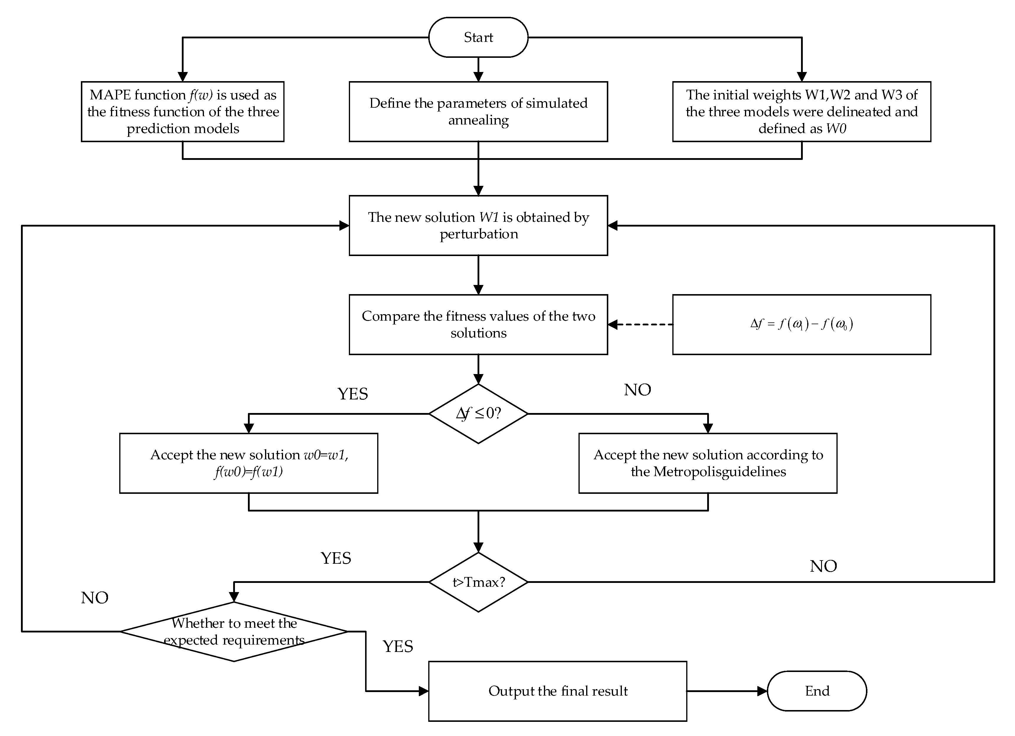
3.11. Simulated Annealing

The SA algorithm can be divided into two parts: the Metropolis criterion and the annealing process. The specific mathematical model is shown in paper [50]. In this paper, the SA algorithm is used to determine the proportion of weights for the prediction results of the three models, and the initial weights of all three models are set to 1/3. Finally, the prediction results of each prediction model are used to determine the final prediction results using Equation (23).

$$Y={\omega }_1{Y}_1+{\omega }_2{Y}_2+{\omega }_3{Y}_3$$

(23)

where $Y$ is the final prediction result; $Y_1$, $Y_2$, and $Y_3$ are the Elman prediction model, CAWOA-ELM prediction model, and EOBL-CSSA-LSSVM prediction model, respectively; and ${\omega }_1$, ${\omega }_2$, and ${\omega }_3$ are the best weighting coefficients for the above three prediction models, respectively. The size of the weights represents the degree of influence the model has on the overall portfolio forecasting model. The larger the weight, the greater the contribution of the model to the portfolio model. The smaller the weight, the smaller the model’s contribution to the portfolio model. The specific operational flow of the SA algorithm to determine the optimal weighting coefficients for the three prediction models is shown in Figure 3.

3.12. The Combined Forecasting Models

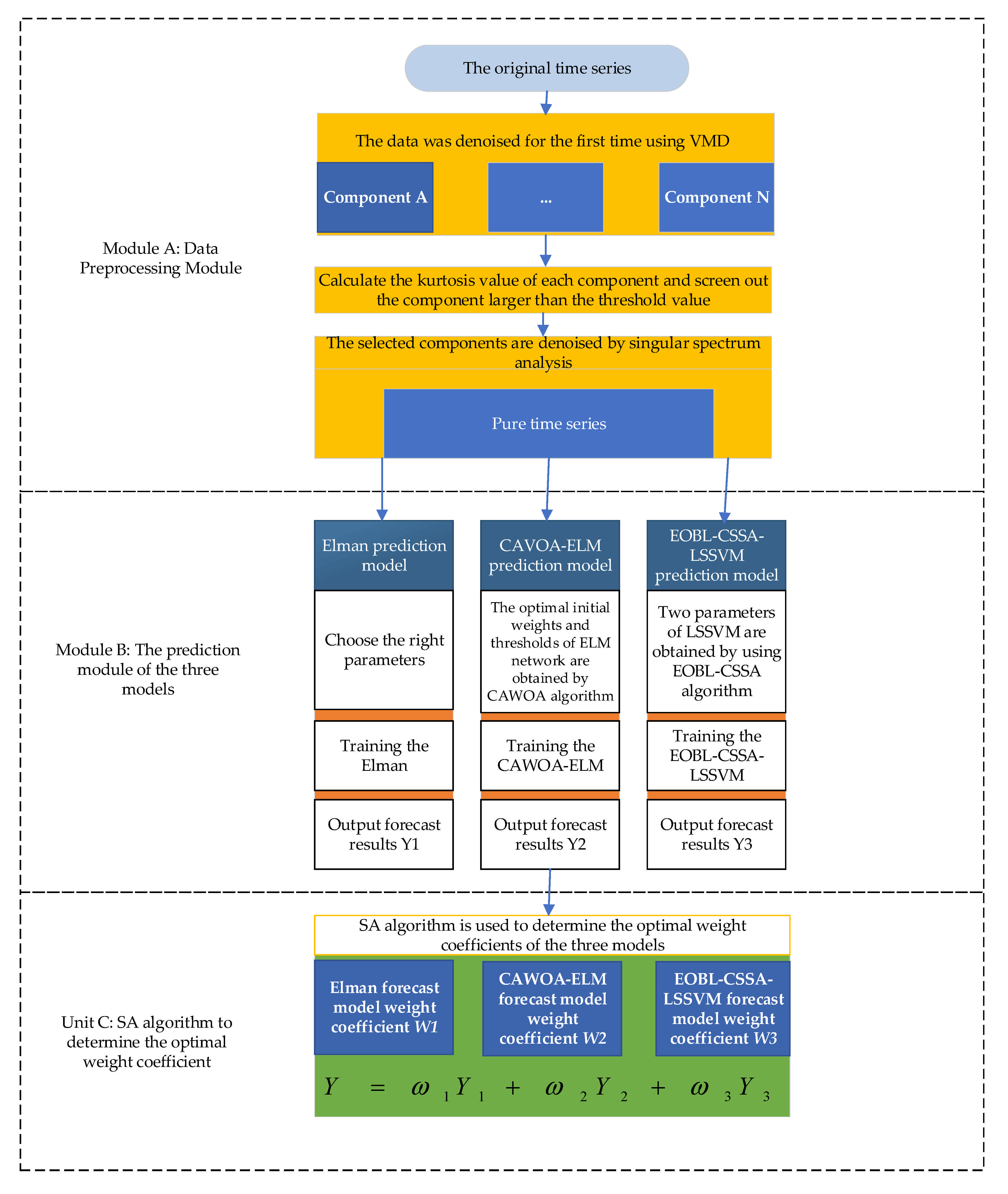
This paper introduces a novel combined prediction model based on machine learning algorithms, swarm intelligence optimization algorithms, and data pre-processing. As shown in Figure 4, the prediction model can be simplified into three modules: Module A, Module B, and Module C.

Module A represents the data processing module. In real life, raw electrical load data inevitably contain data noise. This data noise can significantly interfere with the learning ability of the model. Therefore, we use VMD–spectral analysis to obtain pure signals.

Module B represents the process of obtaining forecasts using three independent forecasting models. Divide the pure data obtained through module A into the input set and the output set. Firstly, the ELMAN prediction model is trained with the dataset and the optimal number of hidden layers is determined by simulation. The prediction results are then recorded as $Y_1$. Secondly, the CAWOA-ELM model is trained with the dataset to obtain the prediction result $Y_2$. The appropriate initial weights and thresholds for the ELM model are selected by the CAWOA algorithm. Thirdly, the EOBL-CSSA-LSSVM model is trained using the dataset to obtain the prediction result $Y_3$. Then, the EOBL-CSSA algorithm is used to optimize the two parameters in the LSSVM: the penalty factor gam and RBF kernel parameter sig.

Module C represents the process of determining the best weighting coefficients for each set of prediction models by using the SA algorithm. Module C represents the weighting calculation process. The SA algorithm is used to determine the best weighting coefficients for each set of predictions obtained from module B predictions. Additionally, the weight coefficients obtained for each set are multiplied with the prediction results of each of the three prediction models. Finally, the final prediction results are obtained by summing.

3.13. Forecast Feedback System for Electricity Load Forecasting Models

In real life, the way in which the electricity load forecasting model is applied is shown in Figure 5. The generator converts the voltage to 220 KV through the booster transformer. The electrical load is then transmitted to the primary high-voltage substation via the 220 KV high-voltage transmission line. The voltage is converted from 220 KV to 110 KV at the primary high-voltage substation and then transmitted to the secondary high-voltage substation via the 110 KV high-voltage transmission line. Finally, the secondary high-voltage substation converts the electrical load to the voltage required by the factory or the general user for the daily supply of electricity. Due to the nature of the electrical load, it cannot be stored on a large scale. If too much of the electrical load is transmitted, it can lead to a waste of resources. If too little electrical load is transmitted, it can lead to inadequate power supply and inconvenience to the population.

Based on the above problems, this paper applies the power load forecasting model to the primary high-voltage substation phase. Firstly, historical data of the power load in the area are collected through the relevant power department. The historical data are applied to the combined forecasting model proposed in this paper. The predictive model learns continuously to accurately predict the values and trends of the power loads on the 110 KV high-voltage transmission lines in the coming days. Secondly, the forecast results are fed back to the relevant authorities to provide accurate and reasonable feedback to the power sector. Finally, the power sector obtains symmetric information through the high accuracy of the combined forecasting model proposed in this paper. This symmetric information will not only help the power sector to maintain a dynamic balance between power supply and consumption, but also to reduce the waste of resources.

4. The Simulation Experiments

4.1. The Datasets

To verify the forecasting performance and applicability of the combined model proposed in this paper, real electricity load data for 20 weeks from 00:00 on 30 April 2007 to 24:00 on 12 September 2007 for the five administrative states of the south-eastern Australian grid are used as the experimental data for the simulation. The experimental data are collected using a 30-min measurement interval. In other words, a total of 48 sets of experimental data are collected each day, making a total of 6720 sets of experimental data. In this paper, electricity load data are divided into seven data subsets in the order of Monday to Sunday. That is, the electricity load data for each Monday of the 20 weeks are stored in the Monday data subset, and so on for the rest, creating a total of seven data subsets from Monday to Sunday. Then, a combined model is built for each data subset for prediction. In this paper, 912 data points from the first 19 weeks of the 20 weeks of data from each data subset are used as the training set and 48 data points from the last week as the test set to verify the prediction performance of the proposed combination model. In this way, each data subset is used to predict the data of the next week using the data of the previous week.

4.2. Error Evaluation Indicators

Because of the uncertainty and randomness of electrical loads, errors are inevitable in any forecasting method. In this paper, the Root Mean Square Error (RMSE), Mean Absolute Percentage Error (MAPE), Mean Square Error (MSE), and Mean Absolute Error (MAE) are used to verify the results. The four evaluation functions are shown in

Table 1. The four error evaluation indicators.

Metrics	The Formula
RMSE	$RMSE=\sqrt{\frac{1}{N}{\displaystyle \sum _{i=1}^N{\left(t_i-p_i\right)}^2}},$
MAPE	$MAPE=\frac{100\%}{N}{\displaystyle \sum _i^N\left|\frac{t_i-p_i}{t_i}\right|},$
MSE	$MSE=\frac{1}{N}{\displaystyle \sum _{i=1}^N{\left(t_i-p_i\right)}^2}$
MAE	$MAE=\frac{1}{N}{\displaystyle \sum _{i=1}^N\left|t_i-p_i\right|},$

where $t_i$ is the i-th sample of expected output; $p_i$ is the i-th sample of predicted output; and $N$ is the sample size.

. In addition, the statistics of the four error evaluation metrics are presented in numerical form to indicate the prediction results of the forecasting model. The lower the value of the statistic, the better the prediction performance.

4.3. Electricity Load Simulation Experiments

4.3.1. Electricity Load Forecasting Data Pre-Processing Experiments

Any noise removal method can only reduce the noise present in the signal as much as possible but cannot remove it completely. In order to verify the noise reduction performance of the VMD–singular spectrum analysis method, in this paper, the data pre-processing simulation comparison experiments are divided into two groups, namely, the VMD–singular spectrum analysis and the singular spectrum analysis method comparison experiments, and the VMD–singular spectrum analysis and the original un-noised method comparison experiments.

In order to better compare the de-noising performance of the VMD–singular spectrum analysis method proposed, the paper is compared with the singular spectrum analysis method used in paper [34] in the comparative test of the de-noising effect.

Model A is the combined forecasting model proposed in paper [34] combining the Jordan, ESN, and LSSVM models. Model B is the novel combined forecasting model proposed in this paper combining the Elman, CAWOA-ELM, and EOBL-CSSA-LSSVM models. In addition, the two combined models are broken down into six single forecasting models for observation and the MAPE values are used as quantitative data. The comparison of noise reduction effect data is shown in

Table 2. VMD–singular spectrum analysis is used in power load denoising reduction experiments (MAPE).

Time	Jordan	PSO-ESN	SA-LSSVM	Combination Model A	Elman	CAWOA-ELM	EOBL-CSSA-LSSVM	Combination Model B
Monday	2.88	1.36	1.02	1.01	1.27	0.97	1.01	0.61
Tuesday	3.26	1.85	1.11	1.03	3.28	1.82	1.09	1.00
Wednesday	2.05	1.13	1.07	0.74	1.42	1.12	1.12	0.81
Thursday	1.79	1.65	1.65	1.41	1.70	1.31	1.00	0.87
Friday	1.21	1.27	0.90	0.62	1.33	0.79	0.64	0.58
Saturday	1.93	1.93	1.06	0.89	1.51	1.03	0.72	0.57
Sunday	2.13	2.39	1.68	1.25	1.85	1.42	0.95	0.79
Average	2.18	1.53	1.21	0.98	1.76	1.20	0.79	0.74

,

Table 3. Singular spectrum analysis is used in power load noise reduction experiments (MAPE).

Time	Jordan	PSO-ESN	SA-LSSVM	Combination Model A	Elman	CAWOA-ELM	EOBL-CSSA-LSSVM	Combination Model B
Monday	2.70	2.04	1.21	1.14	2.01	1.12	1.09	0.82
Tuesday	1.44	2.79	1.39	1.21	2.79	2.47	1.32	1.23
Wednesday	2.03	1.13	2.42	1.02	1.65	1.22	0.97	0.89
Thursday	1.83	1.72	1.26	1.19	2.42	1.37	1.07	0.91
Friday	1.44	1.30	1.03	0.98	1.27	1.26	1.71	1.20
Saturday	2.41	2.48	1.55	1.32	1.86	1.68	1.11	1.08
Sunday	2.26	2.17	1.46	1.29	1.88	1.15	1.23	1.07
Average	2.02	1.95	1.47	1.16	1.98	1.47	1.21	1.02

and

Table 4. Raw data are used for power load noise reduction experiments (MAPE).

Time	Jordan	PSO-ESN	SA-LSSVM	Combination Model A	Elman	CAWOA-ELM	EOBL-CSSA-LSSVM	Combination Model B
Monday	5.02	2.45	1.09	1.32	4.14	1.35	1.02	0.94
Tuesday	6.88	4.07	2.44	2.37	5.02	3.01	1.67	1.53
Wednesday	4.94	1.51	2.80	1.66	3.71	1.74	2.35	1.67
Thursday	3.12	2.95	1.51	1.78	4.45	2.27	1.52	1.48
Friday	5.10	1.66	2.36	1.89	4.88	1.64	2.80	1.57
Saturday	5.47	2.37	4.72	2.35	6.02	2.28	4.42	2.15
Sunday	4.71	1.48	3.16	1.56	6.78	2.79	3.33	2.44
Average	5.03	2.36	2.58	1.85	5.01	2.15	2.44	1.68

.

Through the comparative experimental analysis of the denoising effect of the VMD–singular spectrum analysis and the singular spectrum analysis in Table 2 and Table 3, we can clearly observe that the combined model A has a different degree of reduction in all subsets except for the Thursday subset, where the MAPE value is slightly increased. Among them, the highest reduction in MAPE value is 0.43%, the lowest is 0.13%, and the average prediction error is reduced by 0.18%. For the combined model B, the noise reduction effect of the VMD–spectral analysis was reduced to varying degrees compared to the noise removal effect of the singular spectrum analysis. The highest reduction in MAPE value was 0.62%, the lowest was 0.04%, and the overall average reduction was 0.28%.

In addition, we observed that for the six single combination models, MAPE values decreased to varying degrees for most of the subsets, except for some single models that showed an increase in MAPE values for individual time subsets. Especially for the SA-LSSVM model and the EOSL-CSSA-LSSVM model, the prediction errors are reduced by 0.26% and 0.42%, respectively. Therefore, we can obtain the following conclusion: from the perspective of the overall noise reduction effect, the noise reduction effect of VMD–singular spectrum analysis is better than that of the singular spectrum analysis noise reduction method.

Through the VMD–singular spectrum analysis in Table 2 and Table 4 and the comparative experimental analysis of the original data without denoising, we can observe that, regardless of the combination model A or the combination model B, the effect of noise reduction processing is more obvious, especially for the Elman prediction model and the Jordan prediction model. At the same time, we also observed that almost all the data pre-processed by VMD–singular spectrum analysis in the combined model B have different degrees of reduction in the MAPE value of the unprocessed original data. This also shows that the VMD–singular spectrum noise reduction method does have a positive effect on improving the prediction performance of the combined model. In addition, the highest value of the noise reduction effect is on Sunday, and its MAPE value is reduced by 1.65%. The lowest value of noise reduction effect is on Monday, and its MAPE value is reduced by 0.33%. This may be because the data model of Sunday is more complicated, so the denoising effect is obvious, while the data model of Monday is relatively stable and the noise reduction effect is relatively gentle. In summary, we can draw the conclusion that for the new combined prediction model proposed in this article, the VMD–singular spectrum analysis denoising method can indeed effectively improve the prediction performance of the combined prediction model.

4.3.2. Performance Analysis of Simulation Experiment of Elman Electric Load Forecasting Model

Secondly, Elman forecasting models are built for each of the seven subsets of temporal data divided as described above. In addition, in order to obtain the best predictive performance for the whole combination model, it is necessary to ensure that each sub-model of the combination model achieves the best predictive performance. Since the prediction performance of the Elman network is affected by the number of hidden layers, we ensure that the Elman model achieves the best performance by selecting the appropriate number of hidden layers and choosing a range between 15 and 50. The optimal number of hidden layers for the Elman model is shown in

Table 5. Optimal number of hidden layers in Elman model.

	Monday	Tuesday	Wednesday	Thursday	Friday	Saturday	Sunday
Hidden layer	25	27	25	23	26	32	29
MAPE (%)	1.27	3.28	1.42	1.70	1.33	1.51	1.85

.

As shown in Table 5, the optimal number of hidden layers in the Elman model from the Monday subset to the Friday subset is very similar, and the value fluctuates around 25. Additionally, Monday and Wednesday have the same optimal number of hidden layers. Interestingly, we also found that MAPE values are very similar in all the models except Tuesday. Although the optimal number of hidden layers for Saturday and Sunday is 32 and 37, respectively, the MAPE values for these two subsets are also relatively similar. This may be due to the similarity of the data patterns from Monday to Friday, even though the magnitude of the change in MAPE values is more pronounced on Thursday. We also found that the MAPE values of the ELMAN model fluctuate considerably, and the maximum value is 2.01% of the minimum value.

4.3.3. Performance Analysis of CAWOA-ELM Power Load Forecasting Model

Thirdly, this paper builds seven CAWOA-ELM models for each of the seven data subsets divided above. The performance of the ELM model depends on the initial weights and thresholds. Therefore, we use the CAWOA algorithm to determine the ELM model. In addition, this paper also improves the prediction accuracy of the model by selecting the best hidden layer neurons.

Table 6. The optimal number of hidden layer neurons in CAWOA-ELM model.

	Monday	Tuesday	Wednesday	Thursday	Friday	Saturday	Sunday
Hidden layer	25	24	25	29	42	38	32
MAPE (%)	0.97	1.81	1.12	1.31	0.78	1.03	1.42

shows the optimal number of hidden layers and MAPE values for different datasets. As can be seen from Table 6, the prediction performance of the CAWOA-ELM model is excellent, and the fluctuation of MAPE values is relatively small. The difference between the maximum and minimum values of the MAPE is 1.03%. The difference between the maximum and minimum MAPE values is 1.03%, and the MAPE value for Friday is 0.78%.

4.3.4. Performance Analysis of the EOBL-CSSA-LSSVM Electricity Load Forecasting Model

Finally, seven EOBL-CSSA-LSSVM prediction models are built for each of the seven temporal data subsets divided above. Additionally, the novel EOBL-CSSA algorithm is used to optimize the penalty factor gam and the RBF kernel parameter sig in LSSVM, and the results of the optimization search are shown in

Table 7. The optimization results of EOBL-CSSA algorithm for LSSVM model.

	Monday	Tuesday	Wednesday	Thursday	Friday	Saturday	Sunday
gam	7896.90	10,000.00	9881.20	10,000.00	5712.00	7822.40	6127.30
Sig	153.97	1260.20	31.67	41.10	150.35	30.77	14.44
MAPE (%)	1.01	1.09	1.12	1.00	0.64	0.72	0.95

. Then, the two parameters obtained by the optimization of the EOBL-CSSA algorithm are assigned to the LSSVM prediction model.

4.3.5. SA Algorithm Optimizes the Weighting Factors of Three Electricity Load Forecasting Models

Finally, the SA algorithm is used to solve for the optimal weights for each predictive model in the linear combination formulation. The parameters of the SA algorithm were set as follows: the Markov chain length is 50, the decay parameter is 0.998, and the step factor is 0.01. Moreover, the initial value of the combined weights for all three models was set to 0.33. The optimal weight proportions for each model are shown in

Table 8. The optimized combination weights by the SA algorithm for load forecasting.

	Monday	Tuesday	Wednesday	Thursday	Friday	Saturday	Sunday	Average
W1	0.1175	0.0402	0.2774	0.1761	0.0815	0.0281	0.0386	0.1085
W2	0.5714	0.0961	0.3613	0.3125	0.4473	0.1068	0.0971	0.2846
W3	0.3111	0.8637	0.3613	0.5114	0.4712	0.8651	0.8643	0.6069
MAPE	0.61	1.00	0.81	0.87	0.58	0.57	0.79	0.74

. From Table 8, we find some interesting phenomena: firstly, the average weight of the three models shows that the EOBL-CSSA-LSSVM model has the highest weight and contribution, accounting for approximately 60% of the weight. The Elman model has the lowest weight and contribution, about 10%, while the CAWOA-ELM model also plays a key role, about 30%. Additionally, as shown in the Monday subset, W2 has a weight of 0.5714, while W3 has a weight of 0.5714. This is a good indication that the prediction accuracy of the combined model is influenced in large part by the CAWOA-ELM model. In the Wednesday subset, the weights of the three models are very close to each other, which is a good indication that the three models make similar contributions to the combined model.

Among them, W1 represents the weight of the Elman model, W2 represents the weight of the CAWOA-ELM model, and W3 represents the weight of the EOBL-CSSA-LSSVM model.

5. Analysis of Experimental Results of Power Load Simulation

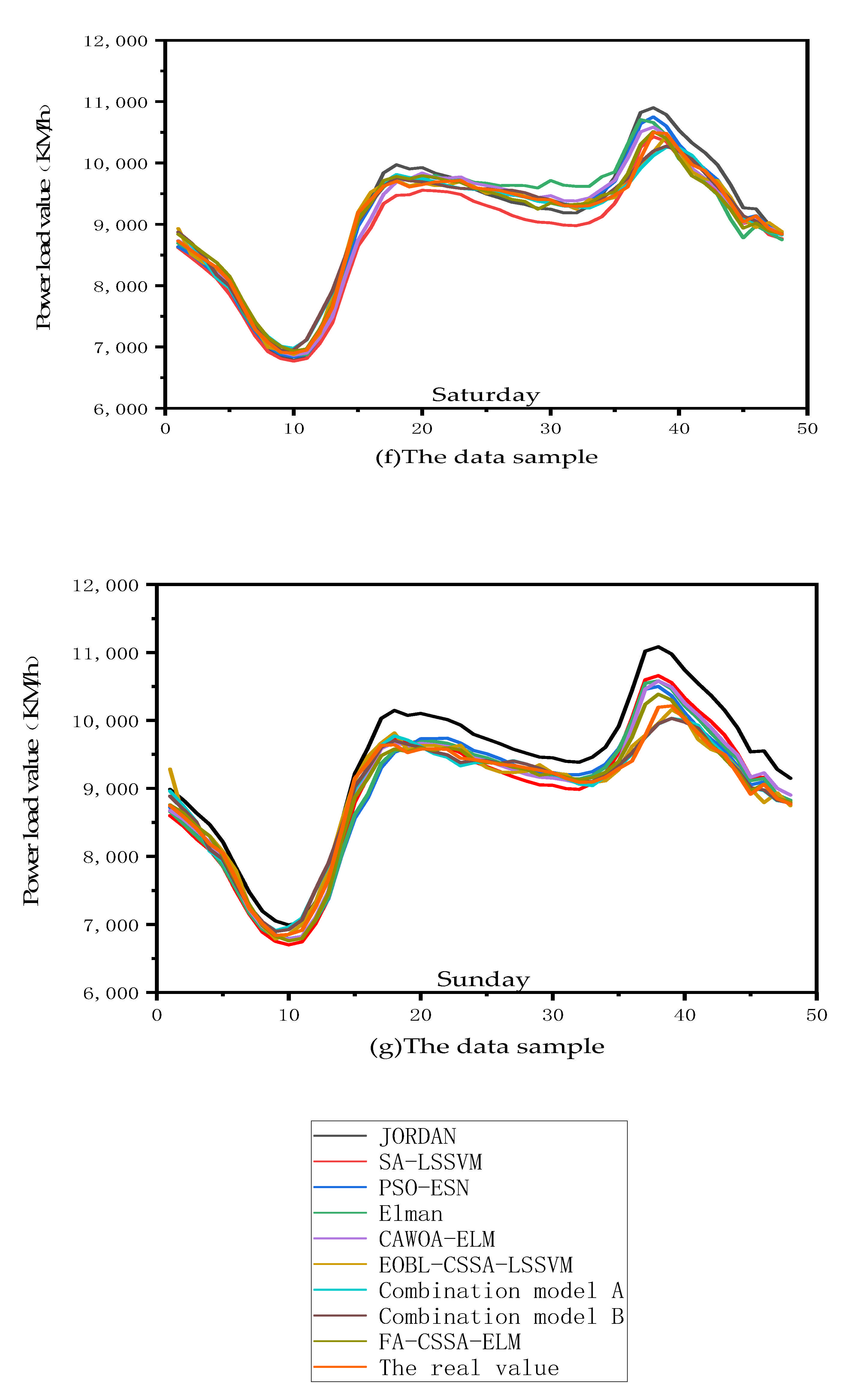
In order to illustrate more effectively the points of the combined prediction model proposed in this paper, we divided the simulation experimental results into several groups of experiments for analysis. Figure 6 shows the prediction results and prediction trends for the three combined prediction models and the six individual prediction models. Figure A1 in Appendix A shows an enlarged view of the prediction results of the competitive model. The three combined forecasting models include the combined forecasting model proposed in this paper, the combined forecasting model proposed in paper [34], and the FA-CSSA-ELM forecasting model proposed in paper [33]. The six individual forecasting models include the Jordan model, the Elman model, the PSO-ESN, the SA-LSSVM, the CAWOA-ELM, and the EOBL-CSSA-LSSVM forecasting model. Additionally, the different color curves represent the prediction results of different prediction models.

We conducted a comparative analysis between the combined prediction model proposed in this paper and the six individual prediction models. As shown in Figure 6, we found that the prediction results of the combined prediction model proposed in this paper are closer to the real historical data. This is followed by the prediction results of the EOBL-CSSA-LSSVM model and the PSO-ESN prediction model. Although the predictive performance of both the EOBL-CSSA-LSSVM model and the PSO-ESN model is excellent, the overall volatility of the PSO-ESN model is higher than that of the EOBL-CSSA-LSSVM model. However, the overall volatility of the PSO-ESN model is higher than that of the EOBL-CSSA-LSSVM model, especially on weekdays. Therefore, we believe that the EOBL-CSSA-LSSVM model has a better predictive performance. In addition, the prediction curves of Jordan’s model and Elman’s model are the furthest away from the real data and have the largest variation. Therefore, we conclude that the prediction performance of the Jordan and Elman models is relatively poor. In summary, the combined prediction model proposed in this paper showed the best prediction accuracy and prediction performance compared to the six individual prediction models.

We also conducted a comparative analysis between the combined prediction model proposed in this paper and the three combined prediction models. As shown in Figure 6, among the three combined prediction models, the FA-CSSA-ELM prediction model has the lowest prediction accuracy and the prediction curve is the farthest away from the real data. In addition, the prediction curves of both the combined prediction model proposed in paper [34] and the prediction model proposed in this paper are very close to the distance of the real data. However, on Thursday, the prediction curves of the model proposed in this paper are closer to the real data. Therefore, from an overall perspective, the prediction model proposed in this paper has the best prediction accuracy.

In order to more intuitively verify the predictive performance of the combined models proposed in this paper, we gave the evaluation values of the different prediction models in numerical form in conjunction with the four error evaluation metrics shown in Table 1, as shown in

Table 9. Evaluation index statistics of different power load competition models.

	Time	Jordan	Elman	PSO-ESN	SA-LSSVM	CAWOA-ELM	EOBL-CSSA-LSSVM	Combination Model A	Combination Model B	FA-CSSA-ELM
MSE	Monday	49.31	21.95	19.38	22.50	16.83	15.62	15.62	10.13	17.09
	Tuesday	50.82	31.45	18.89	51.50	30.13	18.88	17.88	15.22	24.87
	Wednesday	25.51	20.90	17.27	23.45	18.24	17.24	12.10	14.30	16.63
	Thursday	31.57	28.97	27.35	27.65	22.65	17.95	26.24	12.75	13.35
	Friday	18.34	21.68	15.25	23.84	12.30	11.13	10.91	8.72	22.03
	Saturday	33.65	38.12	21.12	30.00	19.96	13.00	14.91	7.95	20.85
	Sunday	35.47	26.43	31.64	33.06	26.86	19.04	21.12	14.28	17.83
MAPE	Monday	2.89	1.36	1.03	1.27	0.97	1.01	1.01	0.61	1.00
	Tuesday	3.27	1.85	1.09	3.28	1.82	1.09	1.03	1.00	1.49
	Wednesday	2.05	1.13	1.07	1.42	1.12	1.12	0.74	0.81	1.02
	Thursday	1.79	1.65	1.65	1.71	1.31	1.01	1.52	0.87	0.94
	Friday	1.21	1.28	0.91	1.33	0.78	0.64	0.62	0.58	1.30
	Saturday	1.93	1.93	1.06	1.51	1.03	0.72	0.90	0.58	1.03
	Sunday	2.13	1.57	1.69	1.85	1.43	0.95	1.26	0.79	0.90
RMSE	Monday	328.56	152.10	134.26	155.88	116.57	112.84	112.84	0.61	118.41
	Tuesday	352.07	235.70	130.85	356.81	230.71	130.82	120.82	74.36	150.76
	Wednesday	128.23	142.80	119.71	162.48	126.37	119.43	80.12	110.42	115.23
	Thursday	218.69	200.71	189.48	191.58	156.93	124.33	197.43	89.76	92.49
	Friday	127.07	150.20	105.69	165.16	85.22	77.12	66.16	91.33	152.65
	Saturday	233.16	264.07	146.34	207.83	138.25	90.09	91.26	57.08	144.48
	Sunday	245.72	183.08	219.18	229.02	186.09	131.90	146.34	54.06	123.56
MAE	Monday	266.73	125.41	98.21	118.17	91.83	87.25	87.25	61.54	96.07
	Tuesday	281.34	158.95	95.95	286.55	155.51	95.95	95.95	96.79	109.62
	Wednesday	99.76	97.21	91.59	122.54	98.53	97.31	66.95	91.55	87.40
	Thursday	150.87	140.69	141.31	145.57	114.11	82.80	144.30	76.96	79.00
	Friday	106.02	115.95	84.13	121.27	68.89	57.95	71.79	67.95	117.4595
	Saturday	179.19	183.82	96.56	141.89	92.43	64.50	79.84	62.89	94.38
	Sunday	191.45	139.69	153.12	167.76	130.51	85.42	96.56	79.10	79.42

. In particular, the RMSE, MSE, and MAE can reflect the prediction accuracy, while the MAPE shows a high prediction expressiveness. In addition, we also compared the prediction performance of different prediction models more visually in the form of bar charts, as shown in Figure 7. From the values of the indicators presented in Table 9 and Figure 7, we found that the RMSE, MAE, MAPE, and MSE values of the combined forecasting model proposed in this paper have the best expressions compared to other competing models. We also found a satisfactory prediction result: the MAPE values for all data subsets were less than or equal to 1%, even with a minimum value of 0.57%. Although the mean MAPE value of the prediction model proposed in paper [34] is very close to 1%, its maximum and minimum MAPE values are 1.52% and 0.62%, respectively. This also indicates that our proposed new combined forecasting model has the best forecasting accuracy and forecasting performance.

6. Conclusions

Nowadays, accurate electrical loads not only help the power sector to make rational work plans and production decisions, but also to reduce the waste of resources and economic losses. Based on the above problems, this paper proposes a combined power load forecasting model based on machine learning, swarm intelligence optimization algorithms, and data pre-processing. The combined model is based on the Elman model, the ELM model, and the LSSVM model. Additionally, two improved swarm intelligence optimization algorithms (CAWOA-CSSA and EOBL-CSSA algorithms) proposed in this paper are used to optimize the parameters of the ELM and LSSVM models, respectively. Then, the SA algorithm is used to calculate and assign the weighting coefficients of the three models. Finally, the final prediction results are obtained by weighted summation. By combining models, the advantages of machine learning algorithms, swarm intelligence optimization algorithms, and data pre-processing can be combined to reduce the shortcomings of a single model. In addition, through several sets of simulations and analysis of the experimental results, we obtained the following conclusions.

• We found that the noise reduction effect of the VMD–singular spectrum analysis method proposed in this paper is obvious and can effectively improve the prediction accuracy of the prediction model. The average MAPE value of the combined prediction model is reduced by 0.28% and the prediction accuracy is improved by 27.4% when compared to the singular spectrum analysis method. The average MAPE value of the combined prediction model is reduced by 0.94% and the prediction accuracy is improved by 55% when compared to the non-denoised method;
• The two improved swarm intelligence optimization algorithms proposed in this paper can improve the prediction accuracy of the combined prediction model. Through Table 8, we can find that the weight proportion of the EOBL-CSSA-LSSVM model is 60% and the weight proportion of the CAWOA-ELM model is 30%, which is good proof that our proposed EOBL-CSSA algorithm and CAWOA-CSSA algorithm play an important role in the combined prediction model;
• The simulation experiments and the analysis of the experimental results show that the combined forecasting model proposed in this paper has the best performance in terms of forecasting performance and forecasting accuracy. The combined model has the best performance in terms of MSE, MAPE, RMSE, and MAE. The prediction model proposed in paper [34] and the FA-CSSA-ELM model proposed in paper [33] are the next best, while the Jordan model has the worst prediction performance. Compared with the Jordan model, the MSE value of the combined model is reduced by 67%, the MAPE value is reduced by 66%, the RMSE value is reduced by 69%, and the MAE value is reduced by 57%. Compared with the FA-CSSA-ELM model, the combined model’s MSE value is reduced by 38%, the MAPE value is reduced by 32%, the RMSE value is reduced by 45%, and the MAE value is reduced by 18%. Compared with paper [34], the MSE value of the combined model is reduced by 31%, the MAPE value is reduced by 32%, the RMSE value is reduced by 33%, and the MAE value is reduced by 15%.

In short, the combined forecasting model proposed in this paper has strong forecasting performance and forecasting accuracy. Additionally, the VMD–singular spectrum analysis method proposed in this paper has an obvious denoising effect. In addition, the EOBL-CSSA algorithm and CAWOA algorithm proposed in this paper can also effectively improve the deficiencies of the machine learning model. Although the predictive performance of our proposed predictive model is excellent, it can provide effective feedback and information for the power sector. However, we have not considered too many practical factors such as weather and holidays. Therefore, we will consider the impact of other factors on power load forecasting in future research.