Path Planning of AS/RS Based on Cost Matrix and Improved Greedy Algorithm

Abstract

Logistics plays an important role in the field of global economy, and the storage and retrieval of tasks in a warehouse which has symmetry is the most important part of logistics. Generally, the shelves of a warehouse have a certain degree of symmetry and similarity in their structure. The storage and retrieval efficiency directly affects the efficiency of logistics. The efficiency of the traditional storage and retrieval mode has become increasingly inconsistent with the needs of the industry. In order to solve this problem, this paper proposes a greedy algorithm based on cost matrix to solve the path planning problem of the automatic storage and retrieval system (AS/RS). Firstly, aiming at the path planning mathematical model of AS/RS, this paper proposes the concept of cost matrix, which transforms the traditional storage and retrieval problem into the element combination problem of cost matrix. Then, a more efficient backtracking algorithm is proposed based on the exhaustive method. After analyzing the performance of the backtracking algorithm, combined with some rules, a greedy algorithm which can further improve efficiency is proposed; the convergence of the improved greedy algorithm is also proven. Finally, through simulation, the time consumption of the greedy algorithm is only 0.59% of the exhaustive method, and compared with the traditional genetic algorithm, the time consumption of the greedy algorithm is about 50% of the genetic algorithm, and it can still maintain its advantage in time consumption, which proves that the greedy algorithm based on cost matrix has a certain feasibility and practicability in solving the path planning of the automatic storage and retrieval system.

1. Introduction

With the development of the global economy, the field of logistics is also developing rapidly. The traditional manual-controlled storage and retrieval scheduling problem does not meet the needs of the times, so the automatic storage and retrieval system (AS/RS) appeared. The AS/RS is an automatic control warehouse system, which can store and retrieve goods automatically in a warehouse which has symmetry instead of manual processing, and is controlled and managed by a computer [1,2]. Generally, the shelves of the warehouse have a certain degree of symmetry and similarity in their structure. A storage and retrieval cycle of tasks usually includes the time of entering and leaving the warehouse, registration time, and storage and retrieval time, among which the storage and retrieval time of goods by the stacker accounts for the largest proportion, and can be as high as 50% of the logistics cycle. If the stacker is not properly dispatched or the dispatching mode is inefficient, the working efficiency of the stacker and the operation efficiency of the entire warehouse will be seriously affected. Therefore, a more reasonable path planning for the storage and retrieval system is the key to improving the efficiency of the stacker [3,4,5].

At present, many scholars have made great achievements in solving the problem of the stacker. Li Ding et al. started with the speed control of the stacker, improved the transport system of the stacker in the automatic warehouse from smooth speed change and accurate parking, and put forward the optimization design of the S-curve algorithm for acceleration and deceleration of the automatic warehouse, so that the stacker can accurately locate goods among the shelves and increase the speed. Speed stability during speed and deceleration ensures the safety and accuracy of goods access [1]. For motion planning of the double stacker, Hisato H. et al. proposed a method to generate a motion path at two levels to avoid collision [6]. Eleonora B. et al. used a genetic algorithm to optimize the distribution of goods in the warehouse and reduce the movement time of the stacker [7]. Of course, since the path planning of the stacker plays an important role in affecting logistics efficiency, more scholars choose to conduct a lot of research on path planning. Sun et al. [8] proposed a new genetic-neural network algorithm to find the optimal path solution for the warehouse assignment problem. Shen Li [9] proposed an improved adaptive genetic algorithm; the dynamic crossover coefficient and variation coefficient are used to not only overcome the shortcomings of premature and slow convergence of the traditional genetic algorithm, but also greatly improve the efficiency of the genetic algorithm. Qiu [10] proposed a scheduling model based on a mixed command sequence. On this basis, an improved chemical reaction optimization (ICRO) algorithm was used to optimize the scheduling path of the dual-stacker. For the position tracking problem of the stacker in an industrial environment, Thakur N., Han C.Y. [11] provided a big data-driven method to study the multimodal components of mobile robot interaction and analyze the data from Bluetooth low-energy (BLE) beacon and BLE scanner, so as to obtain the indoor position of the robot.

Considering the importance of the stacker path planning problem, therefore path planning of AS/RS based on cost matrix and improved greedy algorithm was studied in this paper. In fact, at present, compared with the non-probabilistic algorithm represented by the exhaustive method, more scholars prefer to use a heuristic algorithm represented by the genetic algorithm and ant colony optimization as optimization methods. The main reason is that the solution space of the problem is too large, so the efficiency of the traditional non-probabilistic algorithm is relatively low. However, compared with the heuristic algorithm, the non-probabilistic algorithm does not suffer from fatal problems such as falling into local optimum solution. Therefore, if we try to improve the efficiency of the non-probabilistic algorithm so that it can approach the heuristic algorithm, the comprehensive performance of the non-probabilistic algorithm will be better than the heuristic algorithm, thus providing more alternatives for solving the stacker path planning problem. The purpose of this paper is to propose a greedy algorithm based on cost matrix. Case simulation proves that the method proposed in this paper has excellent efficiency on inheriting the characteristics of the non-probabilistic algorithm which must have the best solution. This makes it possible for the non-probabilistic algorithm to solve the stacker path planning problems.

The purpose of this paper is to propose a greedy algorithm based on cost matrix. Through case simulation, it can be proven that the proposed method inherits the characteristics of the necessary optimal solution of the non-probabilistic algorithm, and its efficiency is also excellent. From the simulation results, its time is far less than that of the exhaustive algorithm and backtracking algorithm; even in the face of the challenge of the traditional genetic algorithm, this algorithm can still keep the advantage of time, which makes it possible for the non-probabilistic algorithm to solve the stacker path problem.

The rest of this paper is organized as follows: Section 2 establishes an abstract model; Section 3 introduces the concept of cost matrix, and based on the law of the backtracking algorithm, a greedy algorithm is proposed to solve the problem. Simulation and results are carried out to verify the feasibility and optimization effect of the proposed algorithm in Section 4. The conclusions and future work are given in Section 5.

2. Problem Description and Model

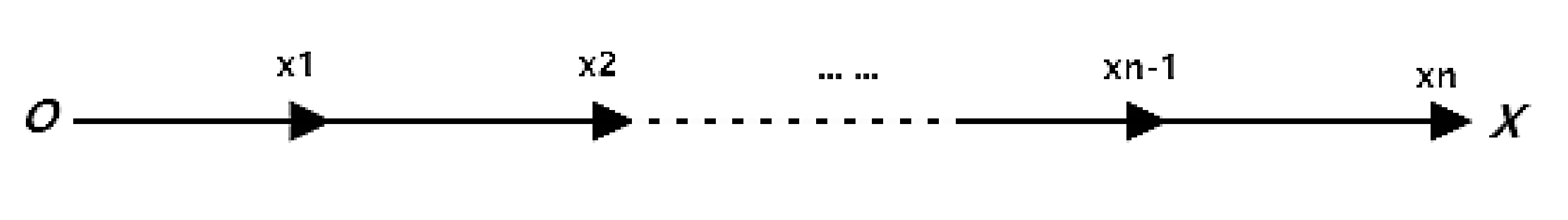
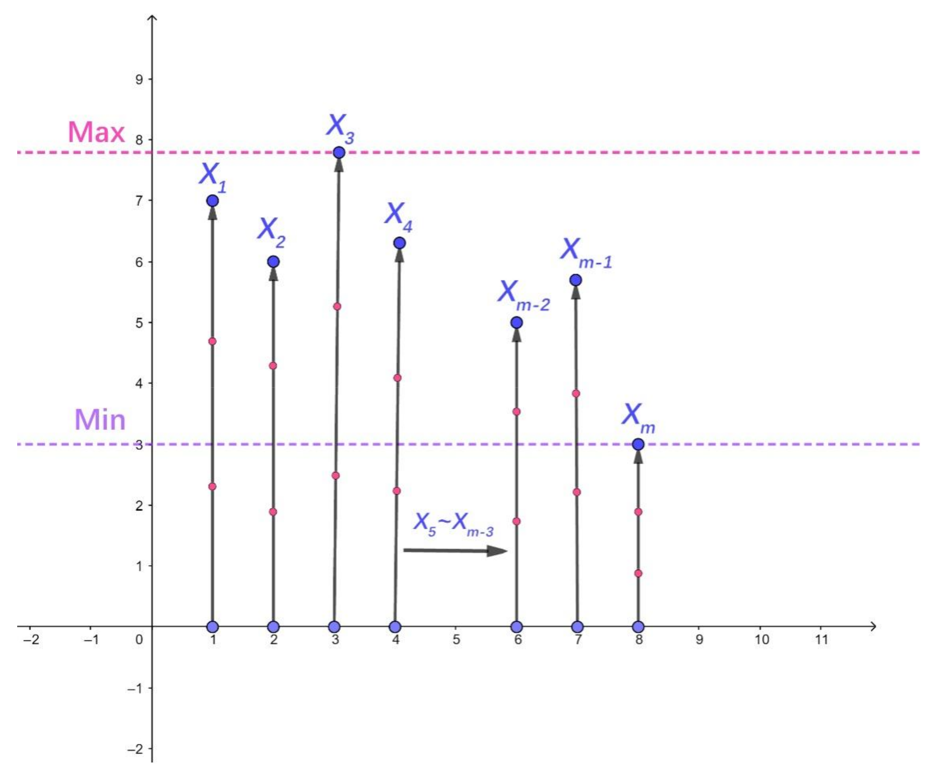
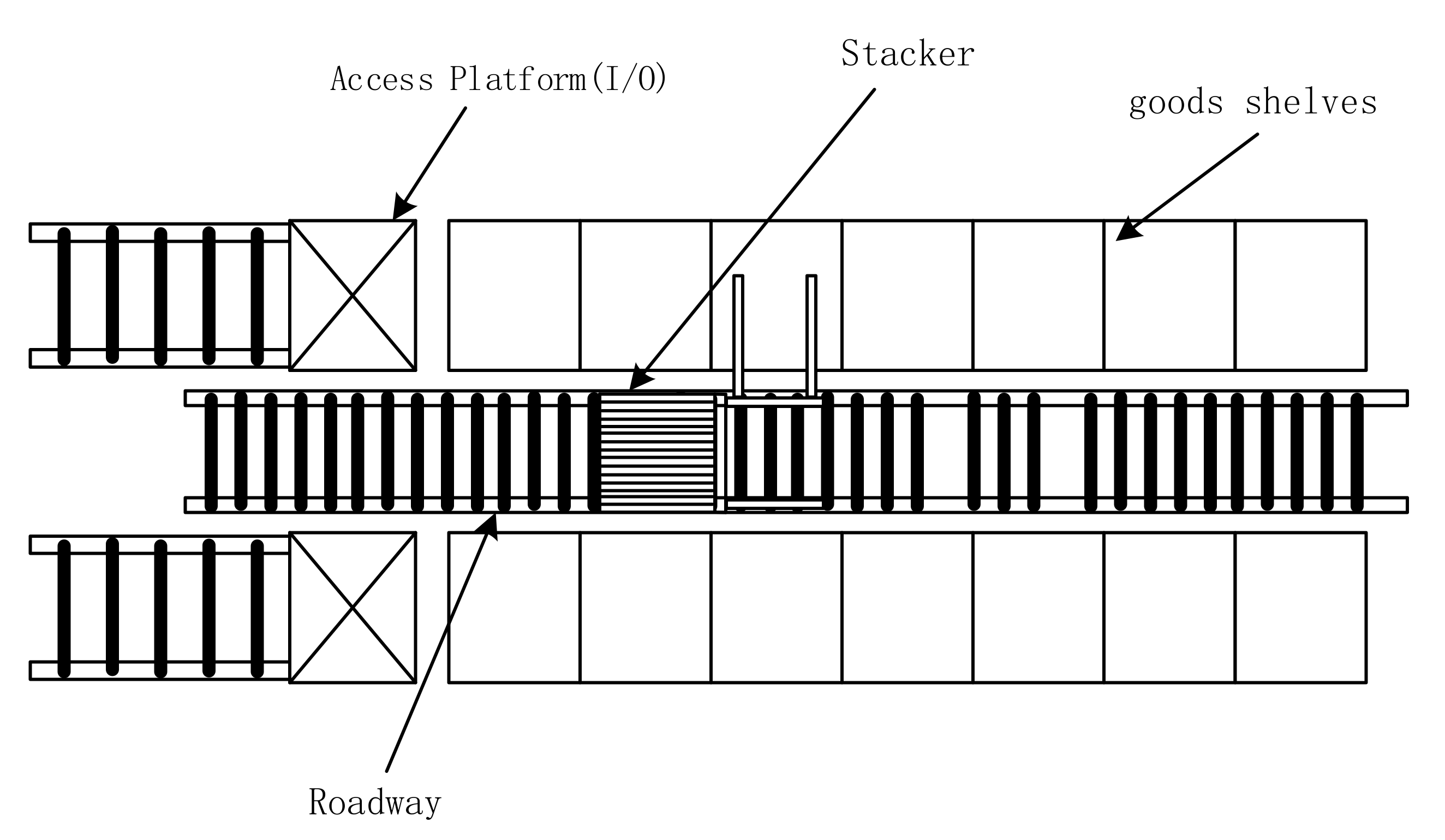
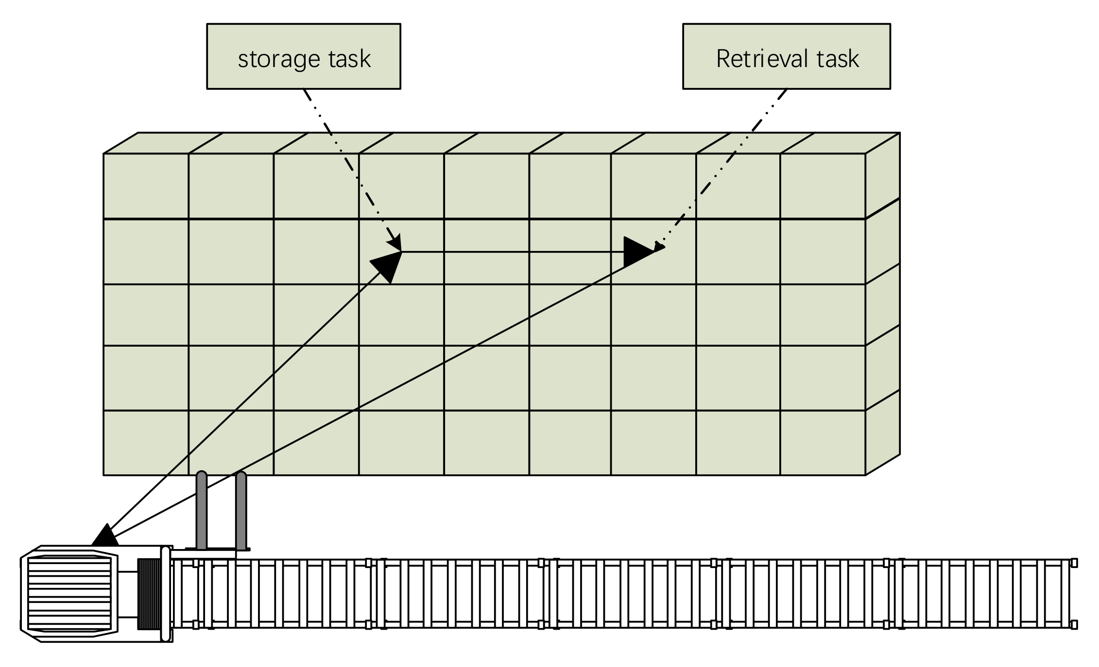
2.1. Problem Description

The objective of this paper is to optimize the path of the stacker in AS/RS. An AS/RS is mainly composed of several storage units, as shown in Figure 1. As for a storage unit, it is mainly composed of access platform, roadway, stacker, and goods shelf [10]. When the system is running, the goods enter and leave the warehouse from the storage platform, and the stacker moving on the roadway moves the goods from the storage platform to the shelf, or takes out the goods from the shelf and transfers them to the storage platform. Whenever the automated warehousing system generates several storage and retrieval tasks, the question of how to determine the optimal operation track of the stacker in the shortest time affects the storage efficiency of the whole system; therefore, this is the problem to be solved in this paper.

2.2. Assumptions

In order to make the model more perfect, a series of assumptions are given as follows:

• Taking a single task as a storage object; that is, the stacker can only deal with one task each time.
• The stacker moves at a constant speed in both horizontal and vertical directions.
• Since the time taken by the stacker to store or take out the goods from the shelf accounts for a small proportion of the total time, this time is ignored; that is, once the stacker moves to the target storage location, it is regarded as completing the storage task.
• All storage units on the shelf have the same length and width.
• The evaluation standard is the total time for the stacker to complete a series of access tasks.

2.3. Variable Table

The symbols used in our model are listed in

Table 1. Symbols and explanations.

Symbol	Explanation
$I_i$	Storage task $(i=1,2,3\dots m)$
$O_j$	Retrieval task $(j=1,2,3\dots n)$
$m$	Number of storage tasks
$n$	Number of retrieval tasks
$L$	Solution sequence model
$S$	Size of solution space
$V_x$	Horizontal moving speed of stacker
$V_y$	Vertical moving speed of stacker
$T$	Total time for stacker to complete task

below.

2.4. Mathematical Model

There are two ways for the stacker to access tasks: (1) when the stacker starts from the I/O station each time, it only executes one retrieval task or storage task, which is called single operation; (2) starting from the I/O station, the stacker first executes a storage task, and then immediately executes a retrieval task, which is called composite operations. Because composite operations can reduce the number of times the stacker moves and improve its operation efficiency, the composite operations mode is considered in this paper.

Assume that there are m storage tasks and n retrieval tasks at the beginning, and assume that the capacity of the stacker is 1; then the solution sequence model L of the solution of the total task is:

$$L=\left\{\begin{array}{ll}{I}_1,O_1,I_2,O_2,\dots ,I_n,O_n,I_{n+1},I_{n+2},\dots ,I_m& ,m>n \\ I_1,O_1,I_2,O_2,\dots ,I_m,O_m,O_{m+1},O_m{}_{+2},\dots ,O_n& ,m<n\end{array}\right.$$

(1)

In Equation (1), $I_i(i=1,2,3\dots m)$ are storage tasks, and $O_j(j=1,2,3\dots n)$ are retrieval tasks, After a brief analysis, it can be seen that $I_1$ has m possibilities, $O_1$ has n possibilities, $I_2$ has m − 1 possibilities, and $O_2$ has n − 1 possibilities… And so on, it is easy to see that the solution space S of L is:

$$S=m\ast n\ast (m-1)\ast (n-1)\ast \dots \ast 1\ast 1=m\ast (m-1)\ast \dots \ast 1\ast n\ast (n-1)\ast \dots \ast 1=m!n!$$

(2)

It can be seen from Equation (2) that the complexity of S for m or n is a factorial level, this means that the application of non-probabilistic algorithms in the stacker path planning problem is limited.

3. Algorithm Design

In this section, this paper firstly proposed a concept of cost matrix, which transforms the original scheduling optimization problem into the element combination problem of cost matrix. Then it was proved that the size of the new solution space is significantly reduced by using the enumeration algorithm. Then, a backtracking algorithm based on the exhaustive method is proposed for optimization, and the simulation results show that the backtracking algorithm can greatly improve the efficiency of the enumeration algorithm. Finally, after analyzing the procession of the backtracking algorithm, we proposed a greedy algorithm to further improve the efficiency of the backtracking algorithm. The simulation results show that the new greedy algorithm is effective.

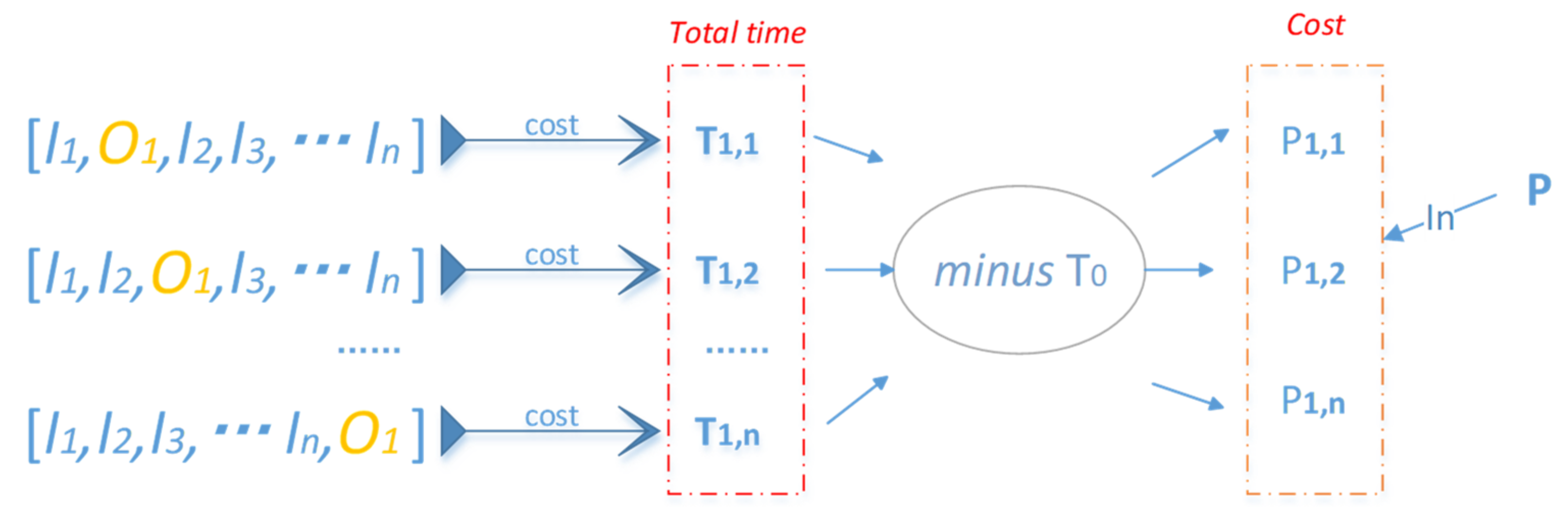
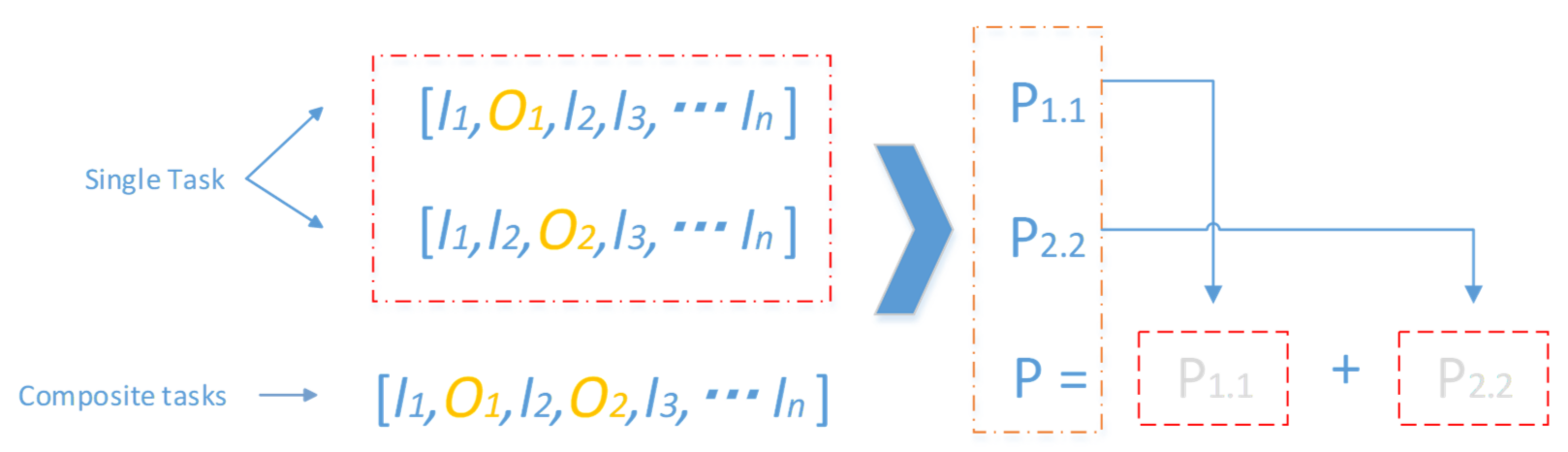
3.1. Cost Matrix

After observing sequence model L in Equation (1), it can be found that at the beginning, I and O appear in pairs, because there is a pair of I/O that forms a loop, as shown in Figure 2.

Therefore, the path in Figure 2 can be looked at as that the stacker starts from the starting point, performs the storage task, and solves a nearby retrieval task at a certain time cost.

Based on the above, the path planning problem of the stacker can be described from another perspective:

Initialize: Suppose that there are n storage tasks $[I_1,I_2,I_3,\dots I_n]$ and m retrieval tasks $[O_1,O_2,O_3,\dots O_m]$.

Step 1: Firstly, only the storage task is considered. Obviously, the total time $T_0$ is a fixed value, as shown in Figure 3.

Step 2-1: Consider only the first retrieval task $O_1$, it can be seen as inserting into a location in the storage task sequence. It is worth noting that the insertion location of $O_1$ will affect the total task time $T_1$, that is $T_1\in [T_{1,1},T_{1,2},\dots ,T_{1,n}]$. By subtracting $T_0$ from $T_{1,1},T_{1,2},\dots ,T_{1,n}$, the generation value corresponding to various schemes can be obtained. Obviously, the generation value can measure the pros and cons of schemes; that is, the cost value $P_{}$ corresponding to the optimal scheme meets $P_{}=\min \{P_{1,1},P_{1,2},\dots ,P_{1,n}\}$, as shown in Figure 4.

Step 2-2: From step 2-1, when only $O_1$ is considered, no matter where $O_1$ is in the task sequence, it always corresponds to a generation value $P_1\in [P_{1,1},P_{1,2},\dots ,P_{1,n}]$. Similarly, when only $O_2$ is considered, there is a generation value $P_2\in [P_{2,1},P_{2,2},\dots ,P_{2,n}]$. When $O_1$ and $O_2$ are considered at the same time, no matter where they are in the task sequence, at this time, the cost value $P_{}$ corresponding to the optimal scheme satisfies Equation (3), and the result is shown in Figure 5.

$$\left\{\begin{array}{l}P=\min \{P_{1,i}+P_{2,j}\}\\ P_{1,i}\in [P_{1,1},P_{1,2},\dots ,P_{1,n}],i=1,2\dots ,n\\ P_{2,j}\in [P_{2,1},P_{2,2},\dots ,P_{2,m}],j=1,2\dots ,m\\ i\ne j\end{array}\right.$$

(3)

Step 3: According to the contents of step 2-1 and step 2-2, by using the analogy method, it can be seen that when all the retrieval tasks $[O_1,O_2,\dots O_m]$ are considered, the cost value $P_{}$ corresponding to the optimal scheme meets the following requirements:

$$\left\{\begin{array}{l}P=\min \{P_{1,i}+P_{2,j}+P_{3,k}+\dots +P_{m,\lambda }\}\\ P_{1,i}\in [P_{1,1},P_{1,2},\dots ,P_{1,n}],i=1,2\dots ,n\\ P_{2,j}\in [P_{2,1},P_{2,2},\dots ,P_{2,n}],j=1,2\dots ,n\\ P_{3,k}\in [P_{3,1},P_{3,2},\dots ,P_{3,n}],k=1,2\dots ,n\\ \dots \dots \\ P_{m,\lambda }\in [P_{m,1},P_{m,2},\dots ,P_{m,n}],\lambda =1,2\dots ,n\\ the i,j,k\dots \lambda \mathrm{is} \mathrm{not} \mathrm{equal}.\end{array}\right.$$

(4)

So far, the path planning problem of the stacker can be transformed into the problem of minimizing the total cost value $P_{}$.

Step 4: The cost matrix C is defined as follows:

$$C=\left[\begin{array}{lllll}{p}_{1,1}& p_{2,1}& p_{3,1}& \dots & p_{m,1}\\ p_{1,2}& p_{2,2}& p_{3,2}& \dots & p_{m,2}\\ \dots & & & & \dots \\ p_{1,n}& p_{2,n}& p_{3,n}& \dots & p_{m,n}\end{array}\right]$$

(5)

where $p_{i,j}$ $(i=1,\dots ,m j=1,\dots ,n)$ is the generation value by binding $O_j$ to $I_i$. So far, the definition of total generation value p is supplemented based on the cost matrix:

$$P={\displaystyle \sum _{k=1}^m{p}_k (p_k\in p_{m,n})}$$

(6)

In Equation (6), any two $p_k$ are not the same row and different columns.

Take any $P_1$ from the first row of the cost matrix C, then delete its row and column, and then take any $P_2$ from the first row of the new C₁, and perform the above operation until $C_{n+1}=\left[ \right]$. After ending a complete traversal sequence, compare the corresponding $P^{\prime }$ value with the known ${P^{\prime }}_{\min }$, if and only if $P^{\prime }$ is less than ${P^{\prime }}_{\min }$, update ${P^{\prime }}_{\min }$ and record the current sequence, and let the corresponding sequence be $P_{\min }$:

$$P_{\min }=P_{i1,j1}+P_{i2,j2}+\dots +P_{in,jn}$$

(7)

The corresponding composite bundling storage and retrieval sequence is:

$$l_1=i_1,j_1,i_2,j_2,\dots ,i_n,j_n$$

(8)

Note that Equation (8) is composed of several pairs of “storage and retrieval” composite tasks. In addition, if no element in column $k_1,k_2\dots$ is selected, the single sequence is:

$$l_2=[1,2,\dots ]$$

(9)

Therefore, the final global sequence is:

$$L=l_1+l_2$$

(10)

The analysis of the above process shows that the solution space of P based on the cost matrix is:

$$S_1=m\ast (m-1)\ast (m-2)\ast \dots \ast 1==m!$$

(11)

It can be obviously seen that S₁ is less than S, it indicates that the model transformation based on cost matrix can effectively reduce the size of solution space.

Next, a simple example is given to illustrate the cost matrix:

Suppose that there are two storage tasks $I_1,I_2$ and two retrieval tasks $O_1,O_2$, and the corresponding shelf coordinates of each task are: $I_1=[5,5]$, $I_2=[10,7]$, $O_1=[6,6]$, $O_2=[11,7]$, the horizontal moving speed $V_x=1 \mathrm{m}/\mathrm{s}$ and the vertical moving speed $V_y=1 \mathrm{m}/\mathrm{s}$ of the stacker.

Obviously, the optimal task sequence should be $L=[I_1,O_1,I_2,O_2]$. Next, we will demonstrate how to get this result through the cost matrix.

From Step 1 above mentioned, it can be seen that only considering the total time $T_0=5+10=15 s$ of the storage tasks, the generation values $P_{1,1}=16-15=1$, $P_{1,2}=15-15=0$, $P_{2,1}=21-15=6$, $P_{2,2}=16-15=1$ can be obtained from step 2-1, and the cost matrix can be obtained according to Equation (5):

$$C=\left[\begin{array}{ll}{P}_{1,1}& P_{2,1}\\ P_{1,2}& P_{2,2}\end{array}\right]=\left[\begin{array}{ll}1& 6\\ 0& 1\end{array}\right]$$

According to Equation (6), when $P=P_{1,1}+P_{2,2}$, $P=P_{\mathrm{m}\mathrm{i}\mathrm{n}}=2$, that means $[I_1,O_1,I_2,O_2]$ is the optimal solution.

3.2. Backtracking Algorithm for Solving Problems

As mentioned above, we only need to find the minimum value of the total cost value p, therefore the backtracking algorithm [12,13] can be used to find $P_{\min }$ by only traversing partial solution space to improve the efficiency of the algorithm.

In the whole process of solving $P_{\min }$, the backtracking algorithm always keeps the known ${P^{\prime }}_{\min }$ as the threshold. In the process of traversing a sequence, if it is found that the cost value $P^{\prime }$ corresponding to the current traversal sequence satisfies the relation $P^{\prime }>{P^{\prime }}_{\min }$, the current traversal is interrupted and the previous node is traced back. Otherwise, after a complete sequence is traversed, let ${P^{\prime }}_{\min }$ be $P^{\prime }$.

The main steps of the backtracking algorithm are as follows:

Step 1. The cost matrix $C$ is constructed based on the existing task data:

$$C=\left[\begin{array}{lllll}{p}_{1,1}& p_{2,1}& p_{3,1}& \dots & p_{m,1}\\ p_{1,2}& p_{2,2}& p_{3,2}& \dots & p_{m,2}\\ \dots & & & & \dots \\ p_{1,n}& p_{2,n}& p_{3,n}& \dots & p_{m,n}\end{array}\right]$$

where $p_{i,j}$ $(i=1,\dots ,m j=1,\dots ,n)$ is the cost value generated by the binding retrieval task $O_j$ to storage task $I_i$. If the time for the stacker to execute only $I_i$ is $t_i$, the time for executing $I_i$ firstly and then $O_j$ on the way is $t_j$, then the corresponding cost value $p_{i,j}=t_j-t_i$. The initial cost value counter $P^{\prime }=0$ and the initial threshold ${P^{\prime }}_{\min }=K$, where $K$ is a number which is larger than the global minimum $P_{\min }$, so $K$ can be taken as follows:

$$K={\displaystyle \sum _{a=1}^n{p}_{a\text{-}max} \left(p_{a\text{-}max} \mathrm{is} \mathrm{the} \mathrm{largest} \mathrm{number} \mathrm{in} \mathrm{row} a\right)}$$

(12)

Finally, the cost matrix $C$ is passed to Step 2.1 for processing.

Step 2: The backtracking algorithm is used to find the minimum value $P_{\min }$ of the total cost value. The specific process is as follows:

Step 2.1: Let the obtained matrix be $C$.

Step 2.1.1: When $C=\left[ \right]$, that is, $C$ is an empty matrix, update ${P^{\prime }}_{\mathrm{m}\mathrm{i}\mathrm{n}}=\mathrm{m}\mathrm{i}\mathrm{n}\{{P^{\prime }}_{\mathrm{m}\mathrm{i}\mathrm{n}},P^{\prime }\}$, and go to Step 2.3 to perform the remaining operations;

Step 2.1.1: When $C$ is a non-empty matrix, take out one element from the first row of the matrix $C$ in turn from left to right, set the element to be taken out as $p_{1,k}$, then calculate the current cost value $P^{\prime }=P^{\prime }+p_{1,k}$, and execute Step 2.2. When all the elements in the first row are taken out once, if the cost matrix $C$ obtained in Step 2.1 comes from Step 1, then directly execute Step 3; otherwise return to Step 2.3 to execute the remaining operations.

Step 2.2: Judge the size of current $P^{\prime }$ and ${P^{\prime }}_{\min }$. If $P^{\prime }\ge {P^{\prime }}_{\min }$, return to Step 2.1 to execute the remaining operations; otherwise, execute Step 2.3.

Step 2.3: The new matrix after deleting row 1 and column K of current matrix C is stored in C₁; then return matrix $C_1$ to Step 2.1 and continue to perform Step 2.1.1 for the remaining operations.

Step 3: Output $P_{\min }$ and corresponding sequence.

The flow chart of backtracking algorithm is shown in Figure 6.

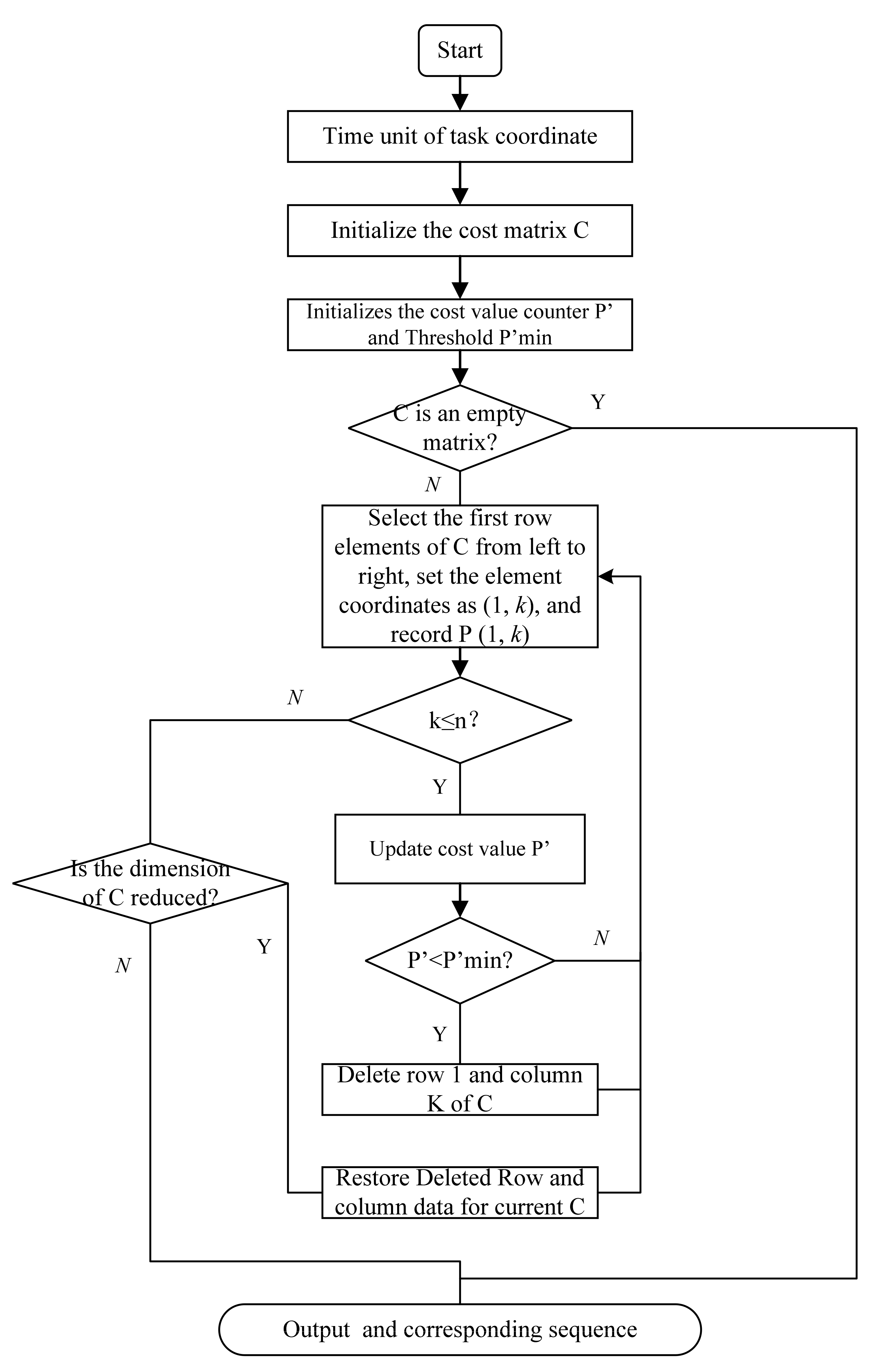
3.3. Greedy Algorithm for Solving Problems

If a sequence vector X is defined, and it is composed of n vectors $x_i(i=1,2,\dots n)$, and any two $x_{i1}$ and $x_{i2}$ satisfy the following condition:

$$\left|x_{i1}\times x_{i2}\right|+\left|x_{i1}·x_{i2}\right|=0$$

(13)

The $X$ diagram is shown in Figure 7:

When the length of $x_i(i=1,2,\dots n)$ is taken as the element size of different rows and columns in the cost matrix $C$, then the length $L_X$ of $X$ is the numerical value of a solution (or a total cost value p), so the solution space of the problem can be regarded as innumerable $X$. If each X is plotted on the x-axis, the solution space is shown in Figure 8.

The analysis shows that the solution space is composed of m Xs in Figure 8, and each X is composed of three $x_i(i=1,2,3)$ (broken by the red dot). Reviewing the logic process of the backtracking algorithm, the traversal process can be regarded as starting from the starting point on x-axis, and continuously jumping up between the red dots until reaching the top, and finding a complete solution. Since the smallest solution X is found, the backtracking algorithm will record the size of the current solution and use it as a threshold. In the following traversal process, after each jump, it is detected whether the current position exceeds the threshold, and the subsequent traversal is abandoned if it exceeds the threshold, as shown in Figure 9.

Therefore, the efficiency of the backtracking algorithm is mainly affected by the threshold. The earlier the threshold approaches the global optimal solution, the higher the optimization efficiency of the algorithm. If and only if the initial threshold is the optimal solution, the optimization efficiency of the backtracking algorithm is the maximum.

Quickly making the threshold approach the global optimal solution is an important way to improve the efficiency of the backtracking algorithm. When the initial threshold is set to the global optimal solution, the characteristics of all nodes below the threshold will be observed. After analyzing, it will be found that the y value of any node is less than the threshold, so it is the global optimal solution. Therefore, a greedy strategy can be designed, which only needs to traverse the node whose y value is lower than the global optimal solution to solve the problem more efficiently [14,15,16,17,18].

Based on the above, a self-locking greedy algorithm is proposed; the steps are as follows:

Step 1: A table group $U_i(i=1,2,3,\dots )$ is defined, in which each $U_i$ table only records the composition of residual solution (or complete solution) nodes whose traversal length is $i$ nodes and the total cost value corresponding to the residual solution (or complete solution). In the initial $U_1$ table, there is residual solution $u_{i=1,j=1}$ (i marks the number of residual solution nodes, j marks the last node of the residual solution as the j-th element of the i-th row element in the cost matrix when it is arranged from small to large).

Step 2: Implement a greedy strategy to traverse the loop.

Step 2.1: Find the solution with the lowest cost value from all tables and name it $u_{i,j}$ (when there are multiple solutions with the same value, the higher i, is the higher priority).

Step 2.1.1: When $u_{i,j}$ is a complete solution; that is, $u_{i,j}$ is in $U_{i_{\max }}$, the greedy algorithm finds the global optimal solution and ends the cycle.

Step 2.1.2: When $u_{i,j}$ is a residual solution, the next node is traversed along $u_{i,j}$, and the new residual solution $u_{i+1,1}$ is put into the corresponding $U_{i+1}$. If $u_{i,j}$ satisfies $u_{i,j=j_{\max }}$, $u_{i,j}$ will be deleted, otherwise $u_{i,j}$ in $U_i$ will be changed to $u_{i,j+1}$. $u_{i+1,1}$ guarantees the inheritance of the optimal solution in $U_i$, and $u_{i,j+1}$ constitutes the self-locking of the inferior quality of the residual solution of $U_i$, which guarantees the deep ergodicity of the superior solution and hinders the invalid ergodicity of the inferior solution.

Step 2.2: Check whether $U_i$ is empty. If it is empty, select the residual solution with the greatest value from $U_{i-1}$ and perform Step 2.1.

Step 3: Output $u_{i,j}$ and the corresponding sequence.

The pseudo codes of the algorithm are shown in Algorithm 1, Algorithm 2 and Algorithm 3:

Algorithm 1 Main program of greedy algorithm

1: init_space()$\stackrel{\hspace{1em}\hspace{1em}}{\to }$ initialize table groups $U_i(i=1,2,3,\dots )$ 2: while true: 3:    smallest_info = seek_the_smallest()$\stackrel{\hspace{1em}\hspace{1em}}{\to }$ find the solution with the least cost value in the table group 4:   r = blossom(smallest_info)$\stackrel{\hspace{1em}\hspace{1em}}{\to }$ update smallest_info and return the status code of the processing result 5:   if r = 1:$\stackrel{\hspace{1em}\hspace{1em}}{\to }$ if smallest_info is the best solution 6:    output smallest_info$\stackrel{\hspace{1em}\hspace{1em}}{\to }$ output results 7:    break $\stackrel{\hspace{1em}\hspace{1em}}{\to }$ Exit the loop and end the program

Algorithm 2 Seek_the_smallest()

1:for i in list_space:$\stackrel{\hspace{1em}\hspace{1em}}{\to }$ Take out all the elements in each table in turn. 2:   Sort all the elements in ascending order according to cost value. 3: for i in list_space: 4:    if there are solutions in the table: 5:     if the cost value of the first solution is less than that of all known: record it 6: return smallest_info $\stackrel{\hspace{1em}\hspace{1em}}{\to }$ Return the solution corresponding to the minimum generation value.

Algorithm 3 Blossom ()
1:	parameter: information of the solution corresponding to the minimum cost value, smallest_ info = [cost value c, layer number of solutions $t$]
2:	if$t$=$i_{\max }$:
3:	return 1
4:	According to smallest_ info find the corresponding solution and write it down as smallest_ solution.
5:	a solution solution_1 in the layer $t+1$ is generated, which satisfies solution_1[“value”] = small_solution[“value”] + value_1, and the row of value_1 is in small_ solution[“next_ available “].
6:	A solution_2 in the $t$ layer is generated, which satisfies the solution_2[“value”], replace the last element of small_solution [“value”] with a slightly larger value in the same column.
7:	return 0

3.4. Proof of Algorithm Convergence to Optimal Solution

As the greedy idea aims to use a series of combinations of local optimal solutions to approximate the global optimal solution, whether the algorithm designed based on the greedy idea can obtain the optimal solution depends on the realization of greedy strategy. Therefore, a proof is carried out by contradiction to the above-designed self-locking greedy algorithm.

Hypothesis: the final output $u_{i1,j1}$ is not the optimal solution.

The optimal solution position currently has the following two cases:

(1) The optimal solution $u_{best}$ is in $U_{i_{\max }}$, which is determined by using Step 2.1 in Section 3.3. Because the cost value of $u_{best}$ is less than $u_{i1,j1}$, the algorithm will give a priority to output $u_{best}$ instead of $u_{i1,j1}$, which is contrary to the assumption, so this situation does not exist.

(2) The optimal solution $u_{best}$ is not completely traversed, but it is located in $U_{i\ne i_{\max }}$ in the form of residual solution $u_{i0,j0}$, assuming that the global optimal solution is $u_{i^{\prime },j^{\prime }}$ and the cost value corresponding to the residual or complete solution in the table group is defined as $P_{i,j}\stackrel{\hspace{1em}f\hspace{1em}}{\leftarrow }{u}_{i,j}$, then the cost value $P_{i^{\prime },j^{\prime }}$ of the optimal solution must be less than $P_{i1,j1}$, and the cost value $P_{i0,j0}$ of the residual solution $u_{i0,j0}$ must be less than $P_{i^{\prime },j^{\prime }}$, that is $P_{i0,j0}<P_{i^{\prime },j^{\prime }}$. According to Step 2.1.2 in Section 3.3, the greedy algorithm always selects $u_{i0,j0}$ for processing; as a result, this situation does not exist.

To sum up, the hypothesis does not hold. Therefore, the self-locking greedy algorithm designed in this paper must be able to find the optimal solution.

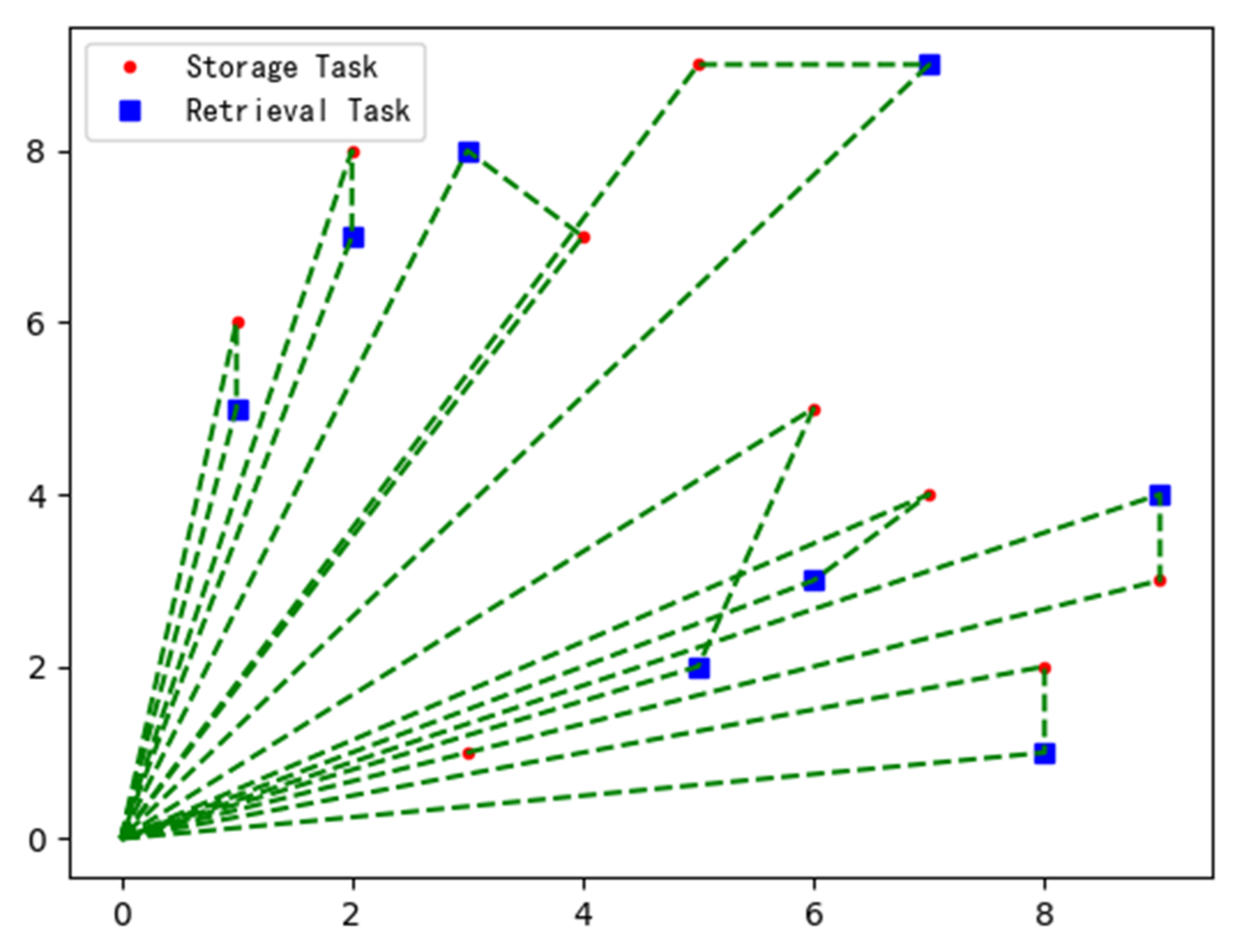
4. Simulation and Results

In this section, a specific example is given to verify the effectiveness of the self-locking greedy algorithm. Suppose there is a three-dimensional warehouse with 9 layers and 10 columns, and there are batch random storage and retrieval tasks, including 9 storage tasks and 8 retrieval tasks. The random tasks are shown in

Table 2. Random task sequence.

Tasks	1	2	3	4	5	6	7	8	9
Storage	(8,2)	(6,5)	(7,4)	(5,9)	(2,8)	(4,7)	(1,6)	(9,3)	(3,1)
Retrieval	(1,5)	(9,4)	(2,7)	(6,3)	(5,2)	(8,1)	(3,8)	(7,9)

.

Using Python language programming, the self-locking greedy algorithm proposed in this paper is verified and simulated on the PC of CPU 2.5 GHz, i5 processor, and is compared with the conventional exhaustive algorithm and backtracking algorithm.

The cost matrix obtained by simulation and the corresponding arrangement of the optimal solution are shown in Figure 10.

It can be seen from Figure 10:

$$P_{\min }=p_{6,0}+p_{7,1}+p_{4,2}+p_{1,3}+\dots +p_{3,7}=8$$

(14)

The task sequence of the stacker is decoded by using Equation (8):

$$l_1=\left[\right[6, 0], [7, 1], [4, 2], [1, 3], [2, 4], [0, 5], [5, 6], [3, 7\left]\right]$$

(15)

Because there is no selected element in column 8, the eighth storage task is a single task command, which is defined by using Equation (9):

$$l_2=[8]$$

(16)

So, the optimal solution sequence is:

$$L=l_1+l_2=\left[\right[6, 0], [7, 1], [4, 2], [1, 3], [2, 4], [0, 5], [5, 6], [3, 7],[8\left]\right]$$

(17)

The total time of task sequence corresponding to the optimal solution according to Equation (4):

$$T=T_I+P_{\min }=118+8=126$$

(18)

The simulation result is shown in Figure 11.

The performance of each algorithm in the simulation process (time, times of selecting behaviors, number of traversing complete sequence) is shown in

Table 3. Comparison of algorithm efficiency.

Algorithm	Time Consuming (s)	Number of Selecting Behaviors (Time)	Number of Traversing Complete Sequence
Exhaustive algorithm	17.9118	623,530	362,880
Backtracking algorithm	0.5588	6172	16
Self-locking greedy algorithm	0.1059	932	1

.

According to the data in Table 3, it takes 17.9118 s for the exhaustive algorithm to traverse the complete solution space, 0.5588 s for the backtracking algorithm to traverse the partial solution space to find the optimal solution, and only 0.1059 s for the greedy algorithm. The time-consuming ratio of greedy algorithm and exhaustive algorithm is ${\delta }_{t1}=\frac{0.1059}{17.9118}=0.59\%$. The time-consuming ratio of greedy algorithm and backtracking algorithm is ${\delta }_{t2}=\frac{0.1059}{0.5588}=18.95\%$. The data in Table 3 also prove that the optimization efficiency of the greedy algorithm can effectively approach the optimal solution that the backtracking algorithm can achieve.

In order to further prove the feasibility of the proposed self-locking greedy algorithm for the stacker path planning problem, the common genetic algorithm (GA) is used in the heuristic algorithms to simulate the above case. The initial parameters of the GA are shown in

Table 4. GA’s parameters.

Parameters	Value
Population size	30
Iterations	100
Mutation probability	0.1
Crossover type	PMX
Selection methods	Tournament selection

.

The simulation result is shown in Figure 12.

It can be seen from Figure 12 that the GA obtains the optimal solution for the first time in the 14th generation, while the total time for running 100 generations is 1.5022 s; that is, the shortest time for GA to obtain the optimal solution is:

$$T_{\min }=\frac{1.5022}{100}\ast 14=0.2103 s$$

(19)

By comparing with Table 3, the time consuming for GA is significantly higher than that of the greedy algorithm. Therefore, it can be proven that the efficiency of the greedy algorithm proposed in this paper is better than that of the general heuristic algorithms.

Considering that the GA is a probabilistic algorithm and the sampled data are probabilistic, therefore ten random simulations are tested by using GA. The optimal solution obtained is Q, the number of iterations for the first optimal solution is R-q. The total running time is T-all, and the time of R-q is T-q. The simulation results are shown in

Table 5. Ten random simulation results.

Times	1	2	3	4	5	6	7	8	9	10
Q	126	126	128	126	128	126	126	126	128	126
R-q	9	11	13	11	15	13	11	14	12	14
T-all	1.85	2.03	1.36	1.65	2.01	2.11	1.47	1.66	1.53	1.54
T-q	0.17	0.22	0.18	0.18	0.30	0.27	0.16	0.23	0.18	0.22

.

It can be seen from the data in Table 5 that the probability of genetic algorithm to obtain the optimal solution is 70%, and the minimum time to obtain the optimal solution is significantly higher than that of the greedy algorithm proposed in this paper. Taking the average value of T-q data in these 10 groups of simulation results as the solution time of traditional genetic algorithm, the time ratio of this self-locking greedy algorithm to traditional genetic algorithm is:

$${\delta }_{t3}=\frac{0.1059}{(0.17+0.22+\dots +0.22)/10}=\frac{0.1059}{0.211}\approx 50.19\%$$

(20)

That is to say, the time of the self-locking greedy algorithm is only half that of the traditional genetic algorithm.

To sum up, the above simulation proves that the combination of greedy algorithm based on cost matrix can play a very good effect; both the optimization speed and the optimization accuracy are better than the performance of the general heuristic algorithm. This makes it possible to apply a non-probabilistic algorithm in solving the stacker path optimization problem.

5. Conclusions

Considering the importance of the path planning of AS/RS, a greedy algorithm based on cost matrix to solve the path planning problem of the AS/RS is proposed. Firstly, aiming at the path planning mathematical model of AS/RS, this paper proposes a concept of cost matrix, which transforms the traditional storage and retrieval problem into the element combination problem of cost matrix. Then, a more efficient backtracking algorithm is proposed based on the exhaustive method. After analyzing the performance of the backtracking algorithm, combined with some rules, a greedy algorithm which can further improve efficiency is proposed; the convergence of the improved greedy algorithm is also verified. Finally, through simulation, the time consumption of the greedy algorithm is only 0.59% of the exhaustive method, and compared with the traditional genetic algorithm, the time consumption of the greedy algorithm is about 50% of the genetic algorithm, and it can still maintain its advantage in time consumption, which proves that the greedy algorithm based on cost matrix has a certain feasibility and practicability in solving the path planning of the automatic storage and retrieval system.

In future research work, the improved greedy algorithm proposed in this paper will be further used to solve job shop scheduling problems, traveling salesman problems, mobile robot path planning problems, etc.

References

- Ding, L.; Chen, Y. Speed Optimization Design of Stacker in Automatic Stereoscopic Warehouse Based on PLC. J. Phys. Conf. Ser. 2020, 1678, 012021. [Google Scholar] [CrossRef]
- Lei, N.N.; Polytechnic, S. Research and application of automatic warehouse system. Mech. Eng. Autom. 2014, 3, 163–165. [Google Scholar]
- Wang, L.; Luo, C. A hybrid genetic tabu search algorithm for mobile robot to solve AS/RS path planning. Int. J. Robot. Autom. 2018, 33, 161–168. [Google Scholar] [CrossRef]
- Hino, H.; Kobayashi, Y.; Higashi, T.; Ota, J. Motion planning method for two stacker cranes in an automated storage and retrieval system. Int. J. Autom. Technol. 2012, 6, 792–801. [Google Scholar] [CrossRef]
- Gao, Q.; Lu, X.W. The complexity and on-line algorithm for automated storage and retrieval system with stacker cranes on one rail. J. Syst. Sci. Complex. 2016, 29, 1302–1319. [Google Scholar] [CrossRef]
- Lu, X.; Shi, H.Y.; Wang, L.; Li, D.W. Analytical travel time models for single and double command of multi-aisle automated storage and retrieval system. Int. J. Manuf. Technol. Manag. 2020, 34, 111–125. [Google Scholar] [CrossRef]
- Bottani, E.; Cecconi, M.; Vignali, G.; Montanari, R. Optimisation of storage allocation in order picking operations through a genetic algorithm. Int. J. Logist. Res. Appl. 2012, 15, 127–146. [Google Scholar] [CrossRef]
- Sun, J.; Zhang, F.; Lu, P.; Yee, J. Optimized modeling and opportunity cost analysis for overloaded interconnected dangerous goods in warehouse operations. Appl. Math. Model. 2021, 90, 151–164. [Google Scholar] [CrossRef]
- Li, S. Path planning of stacker for automated building materials warehouse based on the improved adaptive genetic algorithm. Appl. Mech. Mater. 2013, 325–326, 1475–1478. [Google Scholar] [CrossRef]
- Qiu, J. Research on production scheduling for coordination operation of stackers on monorail. In Proceedings of the 2020 IEEE International Conference on Power, Intelligent Computing and Systems, Shenyang, China, 28–30 July 2020; pp. 901–905. [Google Scholar]
- Thakur, N.; Han, C.Y. Multimodal approaches for indoor localization for ambient assisted living in smart homes. Information 2021, 12, 114. [Google Scholar] [CrossRef]
- Provas, K.R.; Koustav, D. Short term hydro-thermal scheduling using backtracking search algorithm. Int. J. Appl. Metaheuristic Comput. 2020, 11, 38–63. [Google Scholar]
- Yuan, S.; Fu, J.; Cui, F.; Zhang, X. Truck and Trailer Routing Problem Solving by a Backtracking Search Algorithm. J. Syst. Sci. Inf. 2020, 8, 253–272. [Google Scholar] [CrossRef]
- Shao, Z.; Shao, W.; Pi, D. Effective constructive heuristic and iterated greedy algorithm for distributed mixed blocking permutation flow-shop scheduling problem. Knowl. Based Syst. 2021, 221, 106959. [Google Scholar] [CrossRef]
- Chen, S.; Pan, Q.K.; Gao, L. Production scheduling for blocking flowshop in distributed environment using effective heuristics and iterated greedy algorithm. Robot. Comput.-Integr. Manuf. 2021, 71, 1–16. [Google Scholar] [CrossRef]
- Mao, J.-Y.; Pan, Q.-K.; Miao, Z.-H.; Gao, L. An effective multi-start iterated greedy algorithm to minimize makespan for the distributed permutation flowshop scheduling problem with preventive maintenance. Expert Syst. Appl. 2021, 169, 114495. [Google Scholar] [CrossRef]
- Zou, W.Q.; Pan, Q.K.; Tasgetiren, M.F. An effective iterated greedy algorithm for solving a multi-compartment AGV scheduling problem in a matrix manufacturing workshop. Appl. Soft Comput. 2021, 99, 1–17. [Google Scholar] [CrossRef]
- Fehmi, B.O.; Mujgan, S. Iterated greedy algorithms enhanced by hyper-heuristic-based learning for hybrid flexible flowshop scheduling problem with sequence dependent setup times: A case study at a manufacturing plant. Comput. Oper. Res. 2021, 125, 1–15. [Google Scholar]