Some Symmetric Properties and Location Conjecture of Approximate Roots for (p,q)-Cosine Euler Polynomials

Abstract

In this paper, we introduce $(\mathit{p},\mathit{q})$-cosine Euler polynomials. From these polynomials, we find several properties and identities. Moreover, we find the circle equations of approximate roots for $(\mathit{p},\mathit{q})$-cosine Euler polynomials by using a computer.

1. Introduction

To generalize or unify several forms of q-oscillator algebras well-known in the physics literature, many mathematicians introduced $(\mathit{p},\mathit{q})$-number [1,2,3]. As a result, we can find $(\mathit{p},\mathit{q})$-analogues of binomial coefficients, $(\mathit{p},\mathit{q})$-exponential functions, $(\mathit{p},\mathit{q})$-trigonometric functions, and so on, see [2,4,5,6,7,8,9,10]. In this paper, in order to introduce some properties of $(\mathit{p},\mathit{q})$-cosine Euler polynomials, we provide several definitions related to $(\mathit{p},\mathit{q})$-number used in this paper. We begin with notations: $\mathbb{N}$ denotes the set of the natural numbers, $\mathbb{R}$ denotes the set of real numbers and $\mathbb{C}$ denotes the set of complex numbers.

For a natural number n, the $(\mathit{p},\mathit{q})$-number is defined by

$${\left[\mathit{n}\right]}_{\mathit{p},\mathit{q}}=\frac{{\mathit{p}}^{\mathit{n}}-{\mathit{q}}^{\mathit{n}}}{\mathit{p}-\mathit{q}}={\mathit{p}}^{\mathit{n}-1}+{\mathit{p}}^{\mathit{n}-2}\mathit{q}+\cdots +\mathit{p}{\mathit{q}}^{\mathit{n}-2}+{\mathit{q}}^{\mathit{n}-1},$$

which is a natural generalization of the q-number, see [3]. Here, we note that ${\left[\mathit{n}\right]}_{\mathit{p},\mathit{q}}={\left[\mathit{n}\right]}_{\mathit{q},\mathit{p}}$.

Definition 1

(Ref. [5]). For $\mathit{n}\ge \mathit{k}$, the $(\mathit{p},\mathit{q})$-analogues of binomial coefficients are defined by

$${\left[\begin{array}{c}\mathit{n}\\ \mathit{r}\end{array}\right]}_{\mathit{p},\mathit{q}}=\frac{{\left[\mathit{n}\right]}_{\mathit{p},\mathit{q}}!}{{[\mathit{n}-\mathit{k}]}_{\mathit{p},\mathit{q}}!{\left[\mathit{k}\right]}_{\mathit{p},\mathit{q}}!},$$

where m and r are non-negative integers.

We note ${\left[\mathit{n}\right]}_{\mathit{p},\mathit{q}}!={\left[\mathit{n}\right]}_{\mathit{p},\mathit{q}}{[\mathit{n}-1]}_{\mathit{p},\mathit{q}}\cdots {\left[2\right]}_{\mathit{p},\mathit{q}}{\left[1\right]}_{\mathit{p},\mathit{q}}$, where $\mathit{n}\in \mathbb{N}$.

Definition 2

(Ref. [11]). For $\mathit{x}\ne 0$, the $(\mathit{p},\mathit{q})$-derivative of a function f with respect to x is defined by

$${\mathit{D}}_{\mathit{p},\mathit{q}}\mathit{f}\left(\mathit{x}\right)=\frac{\mathit{f}\left(\mathit{p}\mathit{x}\right)-\mathit{f}\left(\mathit{q}\mathit{x}\right)}{(\mathit{p}-\mathit{q})\mathit{x}},$$

and $\left({\mathit{D}}_{\mathit{p},\mathit{q}}\mathit{f}\right)\left(0\right)={\mathit{f}}^{\prime }\left(0\right)$. This proves that f is differentiable at 0, and it is clear that ${\mathit{D}}_{\mathit{p},\mathit{q}}{\mathit{x}}^{\mathit{n}}={\left[\mathit{n}\right]}_{\mathit{p},\mathit{q}}{\mathit{x}}^{\mathit{n}-1}$.

Definition 3

(Refs. [6,12]). The $(\mathit{p},\mathit{q})$-analogue of ${(\mathit{x}+\mathit{a})}^{\mathit{n}}$ is defined by

$${(\mathit{x}\oplus \mathit{a})}_{\mathit{p},\mathit{q}}^{\mathit{n}}=\sum _{\mathit{k}=0}^{\mathit{n}}{\left[\begin{array}{c}\mathit{n}\\ \mathit{k}\end{array}\right]}_{\mathit{p},\mathit{q}}{\mathit{p}}^{\left(\genfrac{}{}{0pt}{}{\mathit{k}}{2}\right)}{\mathit{q}}^{\left(\genfrac{}{}{0pt}{}{\mathit{n}-\mathit{k}}{2}\right)}{\mathit{x}}^{\mathit{k}}{\mathit{a}}^{\mathit{n}-\mathit{k}}.$$

Definition 4

(Ref. [12]). Two forms of $(\mathit{p},\mathit{q})$-exponential functions can be expressed as

$${\mathit{e}}_{\mathit{p},\mathit{q}}\left(\mathit{x}\right)=\sum _{\mathit{n}=0}^{\infty }{\mathit{p}}^{\left(\genfrac{}{}{0pt}{}{\mathit{n}}{2}\right)}\frac{{\mathit{x}}^{\mathit{n}}}{{\left[\mathit{n}\right]}_{\mathit{p},\mathit{q}}!},{\mathit{E}}_{\mathit{p},\mathit{q}}\left(\mathit{x}\right)=\sum _{\mathit{n}=0}^{\infty }{\mathit{q}}^{\left(\genfrac{}{}{0pt}{}{\mathit{n}}{2}\right)}\frac{{\mathit{t}}^{\mathit{n}}}{{\left[\mathit{n}\right]}_{\mathit{p},\mathit{q}}!}.$$

From Definition 4, we can find an important property, ${\mathit{e}}_{\mathit{p},\mathit{q}}\left(\mathit{x}\right){\mathit{E}}_{\mathit{p},\mathit{q}}(-\mathit{x})=1$, see [7,13]. Moreover, U. Duran, M. Acikgos and S. Araci define ${\tilde{\mathit{e}}}_{\mathit{p},\mathit{q}}\left(\mathit{x}\right)$ in [11] as the follows:

$${\tilde{\mathit{e}}}_{\mathit{p},\mathit{q}}\left(\mathit{x}\right)=\sum _{\mathit{n}=0}^{\infty }\frac{{\mathit{x}}^{\mathit{n}}}{{\left[\mathit{n}\right]}_{\mathit{p},\mathit{q}}!}.$$

(1)

From Equation (1) and Definition 4, we can remark

$$\begin{gathered} \left(\mathit{i}\right){\mathit{e}}_{\mathit{p},\mathit{q}}\left(\mathit{x}\right){\mathit{E}}_{\mathit{p},\mathit{q}}\left(\mathit{y}\right)=\sum _{\mathit{n}=0}^{\infty }\frac{{(\mathit{x}\oplus \mathit{y})}_{\mathit{p},\mathit{q}}^{\mathit{n}}}{{\left[\mathit{n}\right]}_{\mathit{p},\mathit{q}}!}={\tilde{\mathit{e}}}_{\mathit{p},\mathit{q}}\left({(\mathit{x}\oplus \mathit{y})}_{\mathit{p},\mathit{q}}\right) \\ \left(\mathit{i}\mathit{i}\right){\mathit{e}}_{\mathit{p},\mathit{q}}\left(\mathit{x}\right){\mathit{E}}_{\mathit{p},\mathit{q}}(-\mathit{y})=\sum _{\mathit{n}=0}^{\infty }\frac{{(\mathit{x}\ominus \mathit{y})}_{\mathit{p},\mathit{q}}^{\mathit{n}}}{{\left[\mathit{n}\right]}_{\mathit{p},\mathit{q}}!}={\tilde{\mathit{e}}}_{\mathit{p},\mathit{q}}\left({(\mathit{x}\ominus \mathit{y})}_{\mathit{p},\mathit{q}}\right) \end{gathered}$$

Definition 5

(Refs. [11,13]). Let $\mathit{i}=\sqrt{-1}\in \mathbb{C}$. Then, the $(\mathit{p},\mathit{q})$-trigonometric functions are defined by

$${\mathit{SIN}}_{\mathit{p},\mathit{q}}\left(\mathit{x}\right)=\frac{{\mathit{E}}_{\mathit{p},\mathit{q}}\left(\mathit{i}\mathit{x}\right)-{\mathit{E}}_{\mathit{p},\mathit{q}}(-\mathit{i}\mathit{x})}{2\mathit{i}}{\mathit{COS}}_{\mathit{p},\mathit{q}}\left(\mathit{x}\right)=\frac{{\mathit{E}}_{\mathit{p},\mathit{q}}\left(\mathit{i}\mathit{x}\right)+{\mathit{E}}_{\mathit{p},\mathit{q}}(-\mathit{i}\mathit{x})}{2},$$

where, ${\mathit{SIN}}_{\mathit{p},\mathit{q}}\left(\mathit{x}\right)={\mathit{sin}}_{{\mathit{p}}^{-1},{\mathit{q}}^{-1}}\left(\mathit{x}\right)$ and ${\mathit{COS}}_{\mathit{p},\mathit{q}}\left(\mathit{x}\right)={\mathit{cos}}_{{\mathit{p}}^{-1},{\mathit{q}}^{-1}}\left(\mathit{x}\right)$.

Such as the same way with their well known Euler expression by means of the exponential functions, we can define the $(\mathit{p},\mathit{q})$-analogues of hyperbolic functions and find some formulae, see [4,11,13].

Theorem 1.

The following relationships hold true.

$$\begin{array}{l}\left(\mathit{i}\right){\mathit{E}}_{\mathit{p},\mathit{q}}\left(\mathit{i}\mathit{t}\mathit{y}\right)=\mathit{C}\mathit{O}{\mathit{S}}_{\mathit{p},\mathit{q}}\left(\mathit{t}\mathit{y}\right)+\mathit{i}\mathit{S}\mathit{I}{\mathit{N}}_{\mathit{p},\mathit{q}}\left(\mathit{t}\mathit{y}\right)\\ \left(\mathit{i}\mathit{i}\right){\mathit{E}}_{\mathit{p},\mathit{q}}(-\mathit{i}\mathit{t}\mathit{y})=\mathit{C}\mathit{O}{\mathit{S}}_{\mathit{p},\mathit{q}}\left(\mathit{t}\mathit{y}\right)-\mathit{i}\mathit{S}\mathit{I}{\mathit{N}}_{\mathit{p},\mathit{q}}\left(\mathit{t}\mathit{y}\right)\end{array}$$

Based on the previous theory, many mathematicians have researched Bernoulli, Euler, and Genocchi polynomials combining $(\mathit{p},\mathit{q})$-numbers. Moreover, they make polynomials of various kinds which have some interesting properties and identities, see [9,12,14,15,16]. We introduce a few polynomials which are needed in this paper.

Definition 6.

For $\left|\mathit{q}\right|<1$ and $\mathit{x},\mathit{y}\in \mathbb{R}$, cosine Euler polynomials ${}_{\mathit{C}}{\mathcal{E}}_{\mathit{n}}(\mathit{x},\mathit{y})$ and q-cosine Euler polynomials ${}_{\mathit{C}}{\mathcal{E}}_{\mathit{n},\mathit{q}}(\mathit{x},\mathit{y})$ are defined respectively as

$$\begin{array}{l}{\displaystyle \sum _{\mathit{n}=0}^{\infty }}{}_{\mathit{C}}{\mathcal{E}}_{\mathit{n}}(\mathit{x},\mathit{y})\frac{{\mathit{t}}^{\mathit{n}}}{\mathit{n}!}=\frac{2}{{\mathit{e}}^{\mathit{t}}+1}{\mathit{e}}^{\mathit{t}\mathit{x}}\mathit{cos}\left(\mathit{t}\mathit{y}\right),\\ {\displaystyle \sum _{\mathit{n}=0}^{\infty }}{}_{\mathit{C}}{\mathcal{E}}_{\mathit{n},\mathit{q}}(\mathit{x},\mathit{y})\frac{{\mathit{t}}^{\mathit{n}}}{{\left[\mathit{n}\right]}_{\mathit{q}}!}=\frac{2}{{\mathit{e}}_{\mathit{q}}\left(\mathit{t}\right)+1}{\mathit{e}}_{\mathit{q}}\left(\mathit{t}\mathit{x}\right)\mathit{C}\mathit{O}{\mathit{S}}_{\mathit{q}}\left(\mathit{t}\mathit{y}\right).\end{array}$$

Definition 7.

Let $|\mathit{p}/\mathit{q}|<1$ and $\mathit{x},\mathit{y}\in \mathbb{R}$. $(\mathit{p},\mathit{q})$-cosine Bernoulli polynomials ${}_{\mathit{C}}{\mathit{B}}_{\mathit{n},\mathit{p},\mathit{q}}(\mathit{x},\mathit{y})$ are defined by

$$\sum _{\mathit{n}=0}^{\infty }{}_{\mathit{C}}{\mathit{B}}_{\mathit{n},\mathit{p},\mathit{q}}(\mathit{x},\mathit{y})\frac{{\mathit{t}}^{\mathit{n}}}{{\left[\mathit{n}\right]}_{\mathit{p},\mathit{q}}!}=\frac{\mathit{t}}{{\mathit{e}}_{\mathit{p},\mathit{q}}\left(\mathit{t}\right)-1}{\mathit{e}}_{\mathit{p},\mathit{q}}\left(\mathit{t}\mathit{x}\right)\mathit{C}\mathit{O}{\mathit{S}}_{\mathit{p},\mathit{q}}\left(\mathit{t}\mathit{y}\right).$$

The different variations of cosine Euler polynomials, q-cosine Euler polynomials and $(\mathit{p},\mathit{q})$-cosine Euler polynomials are illustrated in the diagram below. In addition, Euler polynomials and Bernoulli polynomials are closely related, so in the diagram, we can also see the relationship between cosine Bernoulli polynomials, q-cosine Bernoulli polynomials and $(\mathit{p},\mathit{q})$-Bernoulli polynomials. These research began producing valuable results in areas related to number theory and combinatorics. Mathematicians are studying the extended versions of these polynomials and are researching new polynomials by combining mathematics with other fields, such as physics or engineering.

The aim of this paper is to find some properties and conjectures of $(\mathit{p},\mathit{q})$-cosine Euler polynomials. The contents of the paper are as follows. Section 2 checks the properties of $(\mathit{p},\mathit{q})$-cosine Euler polynomials. For example, we look for $(\mathit{p},\mathit{q})$-differential equations, the properties associated with the symmetric property, and some relations between $(\mathit{p},\mathit{q})$-cosine Euler polynomials and others polynomials. Section 3 identifies the structure and approximate circle of approximate roots of $(\mathit{p},\mathit{q})$-cosine Euler polynomials based on the contents of Section 2.

2. Some Properties of (p, q)-Cosine Euler Polynomials

In this section, we define $(\mathit{p},\mathit{q})$-cosine Euler polynomials using ${\tilde{\mathit{e}}}_{\mathit{p},\mathit{q}}\left(\mathit{x}\right)$. From these polynomials, we find some properties and identities $(\mathit{p},\mathit{q})$-cosine Euler polynomials using $(\mathit{p},\mathit{q})$-binomial coefficients, $(\mathit{p},\mathit{q})$-Cauchy product, and so on.

Definition 8.

Let $0<|\mathit{q}/\mathit{p}|<1$ and $\mathit{x},\mathit{y}\in \mathbb{R}$ with $\mathit{i}=\sqrt{-1}$. Then, we define the generating function of $(\mathit{p},\mathit{q})$-cosine Euler polynomials ${}_{\mathit{C}}{\mathcal{E}}_{\mathit{n},\mathit{p},\mathit{q}}(\mathit{x},\mathit{y})$ as

$$\sum _{\mathit{n}=0}^{\infty }{}_{\mathit{C}}{\mathcal{E}}_{\mathit{n},\mathit{p},\mathit{q}}(\mathit{x},\mathit{y})\frac{{\mathit{t}}^{\mathit{n}}}{{\left[\mathit{n}\right]}_{\mathit{p},\mathit{q}}!}=\frac{2}{{\mathit{e}}_{\mathit{p},\mathit{q}}\left(\mathit{t}\right)+1}{\mathit{e}}_{\mathit{p},\mathit{q}}\left(\mathit{t}\mathit{x}\right)\mathit{C}\mathit{O}{\mathit{S}}_{\mathit{p},\mathit{q}}\left(\mathit{t}\mathit{y}\right).$$

Here, we can note some relations of $(\mathit{p},\mathit{q})$-cosine Euler polynomials, q-cosine Euler polynomials, and cosine Euler polynomials:

(i) $\underset{\mathit{q}\to 1}{lim}{\displaystyle \sum _{\mathit{n}=0}^{\infty }}{}_{\mathit{C}}{\mathcal{E}}_{\mathit{n},1,\mathit{q}}(\mathit{x},\mathit{y})\frac{{\mathit{t}}^{\mathit{n}}}{{\left[\mathit{n}\right]}_{1,\mathit{q}}!}={\displaystyle \sum _{\mathit{n}=0}^{\infty }}{}_{\mathit{C}}{\mathcal{E}}_{\mathit{n}}(\mathit{x},\mathit{y})\frac{{\mathit{t}}^{\mathit{n}}}{\mathit{n}!}=\frac{2}{{\mathit{e}}^{\mathit{t}}+1}{\mathit{e}}^{\mathit{t}\mathit{x}}\mathit{c}\mathit{o}\mathit{s}\left(\mathit{t}\mathit{y}\right)$,

where ${}_{\mathit{C}}{\mathcal{E}}_{\mathit{n}}(\mathit{x},\mathit{y})$ is the cosine Euler polynomials.

(ii) ${\displaystyle \sum _{\mathit{n}=0}^{\infty }}{}_{\mathit{C}}{\mathcal{E}}_{\mathit{n},1,\mathit{q}}(\mathit{x},\mathit{y})\frac{{\mathit{t}}^{\mathit{n}}}{{\left[\mathit{n}\right]}_{1,\mathit{q}}!}={\displaystyle \sum _{\mathit{n}=0}^{\infty }}{}_{\mathit{C}}{\mathcal{E}}_{\mathit{n},\mathit{q}}(\mathit{x},\mathit{y})\frac{{\mathit{t}}^{\mathit{n}}}{{\left[\mathit{n}\right]}_{\mathit{q}}!}=\frac{2}{{\mathit{e}}_{\mathit{q}}\left(\mathit{t}\right)+1}{\mathit{e}}_{\mathit{q}}\left(\mathit{t}\mathit{x}\right)\mathit{C}\mathit{O}{\mathit{S}}_{\mathit{q}}\left(\mathit{t}\mathit{y}\right)$,

where ${}_{\mathit{C}}{\mathcal{E}}_{\mathit{n},\mathit{q}}(\mathit{x},\mathit{y})$ is the q-cosine Euler polynomials.

Theorem 2.

For $|\mathit{q}/\mathit{p}|<1$, we obtain

$${}_{\mathit{C}}{\mathcal{E}}_{\mathit{n},\mathit{p},\mathit{q}}(\mathit{x},\mathit{y})=\sum _{\mathit{k}=0}^{\mathit{n}}{\left[\begin{array}{c}\mathit{n}\\ \mathit{k}\end{array}\right]}_{\mathit{p},\mathit{q}}\frac{{(\mathit{x}\oplus \mathit{i}\mathit{y})}_{\mathit{p},\mathit{q}}^{\mathit{k}}+{(\mathit{x}\ominus \mathit{i}\mathit{y})}_{\mathit{p},\mathit{q}}^{\mathit{k}}}{2}{\mathcal{E}}_{\mathit{n}-\mathit{k},\mathit{p},\mathit{q}},$$

where ${\mathcal{E}}_{\mathit{n},\mathit{p},\mathit{q}}$ is the $(\mathit{p},\mathit{q})$-Euler numbers, see [14].

Proof. 

In [14], we note that

$$\sum _{\mathit{n}=0}^{\infty }{\mathcal{E}}_{\mathit{n},\mathit{p},\mathit{q}}\frac{{\mathit{t}}^{\mathit{n}}}{{\left[\mathit{n}\right]}_{\mathit{p},\mathit{q}}!}=\frac{2}{{\mathit{e}}_{\mathit{p},\mathit{q}}\left(\mathit{t}\right)+1}.$$

We consider ${\mathcal{E}}_{\mathit{n},\mathit{p},\mathit{q}}$ and ${\tilde{\mathit{e}}}_{\mathit{p},\mathit{q}}\left(\mathit{x}\right)$. Substituting ${(\mathit{x}\oplus \mathit{i}\mathit{y})}_{\mathit{p},\mathit{q}}$ instead of x of ${\tilde{\mathit{e}}}_{\mathit{p},\mathit{q}}\left(\mathit{x}\right)$, we find

$$\sum _{\mathit{n}=0}^{\infty }{\mathcal{E}}_{\mathit{n},\mathit{p},\mathit{q}}\frac{{\mathit{t}}^{\mathit{n}}}{{\left[\mathit{n}\right]}_{\mathit{p},\mathit{q}}!}{\tilde{\mathit{e}}}_{\mathit{p},\mathit{q}}\left(\mathit{t}{(\mathit{x}\oplus \mathit{i}\mathit{y})}_{\mathit{p},\mathit{q}}\right)=\frac{2}{{\mathit{e}}_{\mathit{p},\mathit{q}}\left(\mathit{t}\right)+1}{\tilde{\mathit{e}}}_{\mathit{p},\mathit{q}}\left(\mathit{t}{(\mathit{x}\oplus \mathit{i}\mathit{y})}_{\mathit{p},\mathit{q}}\right).$$

(2)

By using $(\mathit{p},\mathit{q})$-analogues of ${(\mathit{x}-\mathit{a})}^{\mathit{n}}$ and a property of ${\tilde{\mathit{e}}}_{\mathit{p},\mathit{q}}\left(\mathit{x}\right)$ in Equation (2), we find

$$\begin{array}{l}{\displaystyle \sum _{\mathit{n}=0}^{\infty }}{\mathcal{E}}_{\mathit{n},\mathit{p},\mathit{q}}\frac{{\mathit{t}}^{\mathit{n}}}{{\left[\mathit{n}\right]}_{\mathit{p},\mathit{q}}!}{\displaystyle \sum _{\mathit{n}=0}^{\infty }}{(\mathit{x}\oplus \mathit{i}\mathit{y})}_{\mathit{p},\mathit{q}}^{\mathit{n}}\frac{{\mathit{t}}^{\mathit{n}}}{{\left[\mathit{n}\right]}_{\mathit{p},\mathit{q}}!}\\ ={\displaystyle \sum _{\mathit{n}=0}^{\infty }}\left({\displaystyle \sum _{\mathit{k}=0}^{\mathit{n}}}{\left[\begin{array}{c}\mathit{n}\\ \mathit{k}\end{array}\right]}_{\mathit{p},\mathit{q}}{(\mathit{x}\oplus \mathit{i}\mathit{y})}_{\mathit{p},\mathit{q}}^{\mathit{k}}{\mathcal{E}}_{\mathit{n}-\mathit{k},\mathit{p},\mathit{q}}\right)\frac{{\mathit{t}}^{\mathit{n}}}{{\left[\mathit{n}\right]}_{\mathit{p},\mathit{q}}!}\\ =\frac{2}{{\mathit{e}}_{\mathit{p},\mathit{q}}\left(\mathit{t}\right)+1}{\mathit{e}}_{\mathit{p},\mathit{q}}\left(\mathit{t}\mathit{x}\right){\mathit{E}}_{\mathit{p},\mathit{q}}\left(\mathit{i}\mathit{t}\mathit{y}\right)\\ =\frac{2}{{\mathit{e}}_{\mathit{p},\mathit{q}}\left(\mathit{t}\right)+1}{\mathit{e}}_{\mathit{p},\mathit{q}}\left(\mathit{t}\mathit{x}\right)(\mathit{C}\mathit{O}{\mathit{S}}_{\mathit{p},\mathit{q}}\left(\mathit{t}\mathit{y}\right)+\mathit{i}\mathit{S}\mathit{I}{\mathit{N}}_{\mathit{p},\mathit{q}}\left(\mathit{t}\mathit{y}\right)).\end{array}$$

(3)

By using Cauchy’s product in the left hand-side of (3), we have

$$\begin{array}{l}{\displaystyle \sum _{\mathit{n}=0}^{\infty }}\left({\displaystyle \sum _{\mathit{k}=0}^{\mathit{n}}}{\left[\begin{array}{c}\mathit{n}\\ \mathit{k}\end{array}\right]}_{\mathit{p},\mathit{q}}{(\mathit{x}\oplus \mathit{i}\mathit{y})}_{\mathit{p},\mathit{q}}^{\mathit{k}}{\mathcal{E}}_{\mathit{n}-\mathit{k},\mathit{p},\mathit{q}}\right)\frac{{\mathit{t}}^{\mathit{n}}}{{\left[\mathit{n}\right]}_{\mathit{p},\mathit{q}}!}\\ =\frac{2}{{\mathit{e}}_{\mathit{p},\mathit{q}}\left(\mathit{t}\right)+1}{\mathit{e}}_{\mathit{p},\mathit{q}}\left(\mathit{t}\mathit{x}\right)(\mathit{C}\mathit{O}{\mathit{S}}_{\mathit{p},\mathit{q}}\left(\mathit{t}\mathit{y}\right)+\mathit{i}\mathit{S}\mathit{I}{\mathit{N}}_{\mathit{p},\mathit{q}}\left(\mathit{t}\mathit{y}\right)).\end{array}$$

(4)

In a similar way, we obtain

$$\begin{array}{l}{\displaystyle \sum _{\mathit{n}=0}^{\infty }}\left({\displaystyle \sum _{\mathit{k}=0}^{\mathit{n}}}{\left[\begin{array}{c}\mathit{n}\\ \mathit{k}\end{array}\right]}_{\mathit{p},\mathit{q}}{(\mathit{x}\ominus \mathit{i}\mathit{y})}_{\mathit{p},\mathit{q}}^{\mathit{k}}{\mathcal{E}}_{\mathit{n}-\mathit{k},\mathit{p},\mathit{q}}\right)\frac{{\mathit{t}}^{\mathit{n}}}{{\left[\mathit{n}\right]}_{\mathit{p},\mathit{q}}!}\\ =\frac{2}{{\mathit{e}}_{\mathit{p},\mathit{q}}\left(\mathit{t}\right)+1}{\mathit{e}}_{\mathit{p},\mathit{q}}\left(\mathit{t}\mathit{x}\right)(\mathit{C}\mathit{O}{\mathit{S}}_{\mathit{p},\mathit{q}}\left(\mathit{t}\mathit{y}\right)-\mathit{i}\mathit{S}\mathit{I}{\mathit{N}}_{\mathit{p},\mathit{q}}\left(\mathit{t}\mathit{y}\right)).\end{array}$$

(5)

From the Equations (4) and (5), we find

$$\begin{array}{l}{\displaystyle \sum _{\mathit{n}=0}^{\infty }}\left({\displaystyle \sum _{\mathit{k}=0}^{\mathit{n}}}{\left[\begin{array}{c}\mathit{n}\\ \mathit{k}\end{array}\right]}_{\mathit{p},\mathit{q}}\left({(\mathit{x}\oplus \mathit{i}\mathit{y})}_{\mathit{p},\mathit{q}}^{\mathit{k}}+{(\mathit{x}\ominus \mathit{i}\mathit{y})}_{\mathit{p},\mathit{q}}^{\mathit{k}}\right){\mathcal{E}}_{\mathit{n}-\mathit{k},\mathit{p},\mathit{q}}\right)\frac{{\mathit{t}}^{\mathit{n}}}{{\left[\mathit{n}\right]}_{\mathit{p},\mathit{q}}!}\\ =2\frac{2}{{\mathit{e}}_{\mathit{p},\mathit{q}}\left(\mathit{t}\right)+1}{\mathit{e}}_{\mathit{p},\mathit{q}}\left(\mathit{t}\mathit{x}\right)\mathit{C}\mathit{O}{\mathit{S}}_{\mathit{p},\mathit{q}}\left(\mathit{t}\mathit{y}\right)\\ =2{\displaystyle \sum _{\mathit{n}=0}^{\infty }}{}_{\mathit{C}}{\mathcal{E}}_{\mathit{n},\mathit{p},\mathit{q}}(\mathit{x},\mathit{y})\frac{{\mathit{t}}^{\mathit{n}}}{{\left[\mathit{n}\right]}_{\mathit{p},\mathit{q}}!},\end{array}$$

which obtain the required result at once. □

Corollary 1.

Setting $\mathit{p}=1$ in Theorem 2, the following holds

$${}_{\mathit{C}}{\mathcal{E}}_{\mathit{n},\mathit{q}}(\mathit{x},\mathit{y})=\sum _{\mathit{k}=0}^{\mathit{n}}{\left[\begin{array}{c}\mathit{n}\\ \mathit{k}\end{array}\right]}_{\mathit{q}}\frac{{(\mathit{x}\oplus \mathit{i}\mathit{y})}_{\mathit{q}}^{\mathit{k}}+{(\mathit{x}\ominus \mathit{i}\mathit{y})}_{\mathit{q}}^{\mathit{k}}}{2}{\mathcal{E}}_{\mathit{n}-\mathit{k},\mathit{q}},$$

where ${}_{\mathit{C}}{\mathcal{E}}_{\mathit{n},\mathit{q}}(\mathit{x},\mathit{y})$ is the q-cosine Euler polynomials.

In [12], authors introduce ${\mathit{C}}_{\mathit{n},\mathit{p},\mathit{q}}(\mathit{x},\mathit{y})$ as the follows.

$${\mathit{e}}_{\mathit{p},\mathit{q}}\left(\mathit{t}\mathit{x}\right)\mathit{C}\mathit{O}{\mathit{S}}_{\mathit{p},\mathit{q}}\left(\mathit{t}\mathit{y}\right)=\sum _{\mathit{n}=0}^{\infty }{\mathit{C}}_{\mathit{n},\mathit{p},\mathit{q}}(\mathit{x},\mathit{y})\frac{{\mathit{t}}^{\mathit{n}}}{{\left[\mathit{n}\right]}_{\mathit{p},\mathit{q}}!}.$$

We note ${\mathit{C}}_{\mathit{n},\mathit{p},\mathit{q}}(\mathit{x},\mathit{y})$ is equal to ${\mathit{C}}_{\mathit{n}}(\mathit{x},\mathit{y})$ when $\mathit{p}=1$ and $\mathit{q}\to 1$, see [15].

Theorem 3.

Let $|\mathit{q}/\mathit{p}|<1$. Then, we find

$${}_{\mathit{C}}{\mathcal{E}}_{\mathit{n},\mathit{p},\mathit{q}}(\mathit{x},\mathit{y})=\sum _{\mathit{k}=0}^{\mathit{n}}{\left[\begin{array}{c}\mathit{n}\\ \mathit{k}\end{array}\right]}_{\mathit{p},\mathit{q}}{\mathcal{E}}_{\mathit{n}-\mathit{k},\mathit{p},\mathit{q}}{\mathit{C}}_{\mathit{k},\mathit{p},\mathit{q}}(\mathit{x},\mathit{y}),$$

where ${\mathcal{E}}_{\mathit{n},\mathit{p},\mathit{q}}$ is the $(\mathit{p},\mathit{q})$-Euler numbers.

Proof. 

From the generation function of the $(\mathit{p},\mathit{q})$-cosine Euler polynomials, we have a relation between ${\mathit{C}}_{\mathit{n},\mathit{p},\mathit{q}}(\mathit{x},\mathit{y})$ and ${\mathcal{E}}_{\mathit{n},\mathit{p},\mathit{q}}$ such as

$$\begin{array}{ll}{\displaystyle \sum _{\mathit{n}=0}^{\infty }}{}_{\mathit{C}}{\mathcal{E}}_{\mathit{n},\mathit{p},\mathit{q}}(\mathit{x},\mathit{y})\frac{{\mathit{t}}^{\mathit{n}}}{{\left[\mathit{n}\right]}_{\mathit{p},\mathit{q}}!}& =\frac{2}{{\mathit{e}}_{\mathit{p},\mathit{q}}\left(\mathit{t}\right)+1}{\mathit{e}}_{\mathit{p},\mathit{q}}\left(\mathit{t}\mathit{x}\right)\mathit{C}\mathit{O}{\mathit{S}}_{\mathit{p},\mathit{q}}\left(\mathit{t}\mathit{y}\right)\\ & ={\displaystyle \sum _{\mathit{n}=0}^{\infty }}{\mathcal{E}}_{\mathit{n},\mathit{p},\mathit{q}}\frac{{\mathit{t}}^{\mathit{n}}}{{\left[\mathit{n}\right]}_{\mathit{p},\mathit{q}}!}\sum _{\mathit{n}=0}^{\infty }{\mathit{C}}_{\mathit{n},\mathit{p},\mathit{q}}(\mathit{x},\mathit{y})\frac{{\mathit{t}}^{\mathit{n}}}{{\left[\mathit{n}\right]}_{\mathit{p},\mathit{q}}!}\\ & ={\displaystyle \sum _{\mathit{n}=0}^{\infty }}\left(\sum _{\mathit{k}=0}^{\mathit{n}}{\left[\begin{array}{c}\mathit{n}\\ \mathit{k}\end{array}\right]}_{\mathit{p},\mathit{q}}{\mathcal{E}}_{\mathit{n}-\mathit{k},\mathit{p},\mathit{q}}{\mathit{C}}_{\mathit{k},\mathit{p},\mathit{q}}(\mathit{x},\mathit{y})\right)\frac{{\mathit{t}}^{\mathit{n}}}{{\left[\mathit{n}\right]}_{\mathit{p},\mathit{q}}!}.\end{array}$$

(6)

By comparing the coefficients of both-sides in Equation (6), we derive the required result. □

Corollary 2.

Putting $\mathit{p}=1$ in Theorem 3, one holds

$${}_{\mathit{C}}{\mathcal{E}}_{\mathit{n},\mathit{q}}(\mathit{x},\mathit{y})=\sum _{\mathit{k}=0}^{\mathit{n}}{\left[\begin{array}{c}\mathit{n}\\ \mathit{k}\end{array}\right]}_{\mathit{q}}{\mathcal{E}}_{\mathit{n}-\mathit{k},\mathit{q}}{\mathit{C}}_{\mathit{k},\mathit{q}}(\mathit{x},\mathit{y}),$$

where ${}_{\mathit{C}}{\mathcal{E}}_{\mathit{n},\mathit{q}}(\mathit{x},\mathit{y})$ is the q-cosine Euler polynomials, ${\mathcal{E}}_{\mathit{n},\mathit{q}}$ is the q-Euler numbers, and ${\sum }_{\mathit{n}=0}^{\infty }{\mathit{C}}_{\mathit{n},\mathit{q}}(\mathit{x},\mathit{y})\frac{{\mathit{t}}^{\mathit{n}}}{{\left[\mathit{n}\right]}_{\mathit{q}}!}={\mathit{e}}_{\mathit{q}}\left(\mathit{t}\mathit{x}\right)\mathit{C}\mathit{O}{\mathit{S}}_{\mathit{q}}\left(\mathit{t}\mathit{y}\right)$.

Theorem 4.

Let ${\mathit{e}}_{\mathit{p},\mathit{q}}\left(\mathit{t}\right)\ne -1$ and $|\mathit{q}/\mathit{p}|<1$. Then, we obtain

$${\mathit{C}}_{\mathit{n},\mathit{p},\mathit{q}}(\mathit{x},\mathit{y})=\frac{1}{2}\left(\sum _{\mathit{k}=0}^{\mathit{n}}{\left[\begin{array}{c}\mathit{n}\\ \mathit{k}\end{array}\right]}_{\mathit{n},\mathit{q}}{\mathit{p}}^{\left(\genfrac{}{}{0pt}{}{\mathit{n}-\mathit{k}}{2}\right)}{}_{\mathit{C}}{\mathcal{E}}_{\mathit{k},\mathit{p},\mathit{q}}(\mathit{x},\mathit{y})+{}_{\mathit{C}}{\mathcal{E}}_{\mathit{n},\mathit{p},\mathit{q}}(\mathit{x},\mathit{y})\right).$$

Proof. 

If we suppose ${\mathit{e}}_{\mathit{p},\mathit{q}}\left(\mathit{t}\right)\ne -1$ for $(\mathit{p},\mathit{q})$-cosine Euler polynomials, then we have

$$\sum _{\mathit{n}=0}^{\infty }{}_{\mathit{C}}{\mathcal{E}}_{\mathit{n},\mathit{p},\mathit{q}}(\mathit{x},\mathit{y})\frac{{\mathit{t}}^{\mathit{n}}}{{\left[\mathit{n}\right]}_{\mathit{p},\mathit{q}}!}({\mathit{e}}_{\mathit{p},\mathit{q}}\left(\mathit{t}\right)+1)=2{\mathit{e}}_{\mathit{p},\mathit{q}}\left(\mathit{t}\mathit{x}\right)\mathit{C}\mathit{O}{\mathit{S}}_{\mathit{p},\mathit{q}}\left(\mathit{t}\mathit{y}\right)$$

(7)

By using the power series of ${\mathit{e}}_{\mathit{p},\mathit{q}}\left(\mathit{t}\right)$ and Cauchy’s product in Equation (7), we find

$$\begin{array}{l}{\displaystyle \sum _{\mathit{n}=0}^{\infty }}{}_{\mathit{C}}{\mathcal{E}}_{\mathit{n},\mathit{p},\mathit{q}}(\mathit{x},\mathit{y})\frac{{\mathit{t}}^{\mathit{n}}}{{\left[\mathit{n}\right]}_{\mathit{p},\mathit{q}}!}({\mathit{e}}_{\mathit{p},\mathit{q}}\left(\mathit{t}\right)+1)\\ ={\displaystyle \sum _{\mathit{n}=0}^{\infty }}{}_{\mathit{C}}{\mathcal{E}}_{\mathit{n},\mathit{p},\mathit{q}}(\mathit{x},\mathit{y})\frac{{\mathit{t}}^{\mathit{n}}}{{\left[\mathit{n}\right]}_{\mathit{p},\mathit{q}}!}\left({\displaystyle \sum _{\mathit{n}=0}^{\infty }}{\mathit{p}}^{\left(\genfrac{}{}{0pt}{}{\mathit{n}}{2}\right)}\frac{{\mathit{t}}^{\mathit{n}}}{{\left[\mathit{n}\right]}_{\mathit{p},\mathit{q}}!}+1\right)\\ ={\displaystyle \sum _{\mathit{n}=0}^{\infty }}\left({\displaystyle \sum _{\mathit{k}=0}^{\mathit{n}}}{\left[\begin{array}{c}\mathit{n}\\ \mathit{k}\end{array}\right]}_{\mathit{p},\mathit{q}}{\mathit{p}}^{\left(\genfrac{}{}{0pt}{}{\mathit{n}-\mathit{k}}{2}\right)}{}_{\mathit{C}}{\mathcal{E}}_{\mathit{k},\mathit{p},\mathit{q}}(\mathit{x},\mathit{y})+{}_{\mathit{C}}{\mathcal{E}}_{\mathit{n},\mathit{p},\mathit{q}}(\mathit{x},\mathit{y})\right)\frac{{\mathit{t}}^{\mathit{n}}}{{\left[\mathit{n}\right]}_{\mathit{p},\mathit{q}}!}\\ =2{\displaystyle \sum _{\mathit{n}=0}^{\infty }}{\mathit{C}}_{\mathit{n},\mathit{p},\mathit{q}}(\mathit{x},\mathit{y})\frac{{\mathit{t}}^{\mathit{n}}}{{\left[\mathit{n}\right]}_{\mathit{p},\mathit{q}}!}.\end{array}$$

(8)

We complete the proof of Theorem 4 from Equation (8). □

In [12], we can find a relation between ${\mathit{C}}_{\mathit{n},\mathit{p},\mathit{q}}(\mathit{x},\mathit{y})$ and ${}_{\mathit{C}}{\mathit{B}}_{\mathit{n},\mathit{p},\mathit{q}}(\mathit{x},\mathit{y})$ as

$${\left[\mathit{n}\right]}_{\mathit{p},\mathit{q}}{\mathit{C}}_{\mathit{n}-1,\mathit{p},\mathit{q}}(\mathit{x},\mathit{y})=\sum _{\mathit{k}=0}^{\mathit{n}-1}{\left[\begin{array}{c}\mathit{n}\\ \mathit{k}\end{array}\right]}_{\mathit{p},\mathit{q}}{\mathit{p}}^{\left(\genfrac{}{}{0pt}{}{\mathit{n}-\mathit{k}}{2}\right)}{}_{\mathit{C}}{\mathit{B}}_{\mathit{k},\mathit{p},\mathit{q}}(\mathit{x},\mathit{y})-{}_{\mathit{C}}{\mathit{B}}_{\mathit{n},\mathit{p},\mathit{q}}(\mathit{x},\mathit{y}),$$

(9)

where ${}_{\mathit{C}}{\mathit{B}}_{\mathit{n},\mathit{p},\mathit{q}}(\mathit{x},\mathit{y})$ is the $(\mathit{p},\mathit{q})$-cosine Bernoulli polynomials.

Corollary 3.

From the Theorem 4 and Equation (9), we find a relation such as

$$\begin{array}{l}{\displaystyle \sum _{\mathit{k}=0}^{\mathit{n}}}{\left[\begin{array}{c}\mathit{n}+1\\ \mathit{k}\end{array}\right]}_{\mathit{p},\mathit{q}}{\mathit{p}}^{\left(\genfrac{}{}{0pt}{}{\mathit{n}+1-\mathit{k}}{2}\right)}{}_{\mathit{C}}{\mathit{B}}_{\mathit{k},\mathit{p},\mathit{q}}(\mathit{x},\mathit{y})-{}_{\mathit{C}}{\mathit{B}}_{\mathit{n},\mathit{p},\mathit{q}}(\mathit{x},\mathit{y})\\ =\frac{{[\mathit{n}+1]}_{\mathit{p},\mathit{q}}}{2}\left({\displaystyle \sum _{\mathit{k}=0}^{\mathit{n}}}{\left[\begin{array}{c}\mathit{n}\\ \mathit{k}\end{array}\right]}_{\mathit{p},\mathit{q}}{\mathit{p}}^{\left(\genfrac{}{}{0pt}{}{\mathit{n}-\mathit{k}}{2}\right)}{}_{\mathit{C}}{\mathcal{E}}_{\mathit{k},\mathit{p},\mathit{q}}(\mathit{x},\mathit{y})+{}_{\mathit{C}}{\mathcal{E}}_{\mathit{n},\mathit{p},\mathit{q}}(\mathit{x},\mathit{y})\right),\end{array}$$

where ${}_{\mathit{C}}{\mathit{B}}_{\mathit{n},\mathit{p},\mathit{q}}(\mathit{x},\mathit{y})$ is the $(\mathit{p},\mathit{q})$-cosine Bernoulli polynomials, see [12].

Theorem 5.

For $|\mathit{q}/\mathit{p}|<1$, we find

$${}_{\mathit{C}}{\mathcal{E}}_{\mathit{n},\mathit{p},\mathit{q}}(1,\mathit{y})=\sum _{\mathit{k}=0}^{\mathit{n}}{\left[\begin{array}{c}\mathit{n}\\ \mathit{k}\end{array}\right]}_{\mathit{p},\mathit{q}}{(-1)}^{\mathit{n}-\mathit{k}}(2{\mathit{C}}_{\mathit{k},\mathit{p},\mathit{q}}(\mathit{x},\mathit{y})-{}_{\mathit{C}}{\mathcal{E}}_{\mathit{k},\mathit{p},\mathit{q}}(\mathit{x},\mathit{y})){\mathit{q}}^{\left(\genfrac{}{}{0pt}{}{\mathit{n}-\mathit{k}}{2}\right)}{\mathit{x}}^{\mathit{n}-\mathit{k}}.$$

Proof. 

Put $\mathit{x}=1$ in the generating function of $(\mathit{p},\mathit{q})$-Euler polynomials. Then, we find

$$\sum _{\mathit{n}=0}^{\infty }{}_{\mathit{C}}{\mathcal{E}}_{\mathit{n},\mathit{p},\mathit{q}}(1,\mathit{y})\frac{{\mathit{t}}^{\mathit{n}}}{{\left[\mathit{n}\right]}_{\mathit{p},\mathit{q}}!}=2\mathit{C}\mathit{O}{\mathit{S}}_{\mathit{p},\mathit{q}}\left(\mathit{t}\mathit{y}\right)-\frac{2}{{\mathit{e}}_{\mathit{p},\mathit{q}}\left(\mathit{t}\right)+1}\mathit{C}\mathit{O}{\mathit{S}}_{\mathit{p},\mathit{q}}\left(\mathit{t}\mathit{y}\right)$$

(10)

By applying $1={\mathit{e}}_{\mathit{p},\mathit{q}}\left(\mathit{x}\right){\mathit{E}}_{\mathit{p},\mathit{q}}(-\mathit{x})$ in Equation (10), we derive

$$\begin{array}{l}{\displaystyle \sum _{\mathit{n}=0}^{\infty }}{}_{\mathit{C}}{\mathcal{E}}_{\mathit{n},\mathit{p},\mathit{q}}(1,\mathit{y})\frac{{\mathit{t}}^{\mathit{n}}}{{\left[\mathit{n}\right]}_{\mathit{p},\mathit{q}}!}\\ =\left(2{\mathit{e}}_{\mathit{p},\mathit{q}}\left(\mathit{t}\mathit{x}\right)\mathit{C}\mathit{O}{\mathit{S}}_{\mathit{p},\mathit{q}}\left(\mathit{t}\mathit{y}\right)-\frac{2}{{\mathit{e}}_{\mathit{p},\mathit{q}}\left(\mathit{t}\right)+1}{\mathit{e}}_{\mathit{p},\mathit{q}}\left(\mathit{t}\mathit{x}\right)\mathit{C}\mathit{O}{\mathit{S}}_{\mathit{p},\mathit{q}}\left(\mathit{t}\mathit{y}\right)\right){\mathit{E}}_{\mathit{p},\mathit{q}}(-\mathit{x})\\ ={\displaystyle \sum _{\mathit{n}=0}^{\infty }}\left({\displaystyle \sum _{\mathit{k}=0}^{\mathit{n}}}{\left[\begin{array}{c}\mathit{n}\\ \mathit{k}\end{array}\right]}_{\mathit{p},\mathit{q}}{(-1)}^{\mathit{n}-\mathit{k}}{\mathit{q}}^{\left(\genfrac{}{}{0pt}{}{\mathit{n}-\mathit{k}}{2}\right)}(2{\mathit{C}}_{\mathit{k},\mathit{p},\mathit{q}}(\mathit{x},\mathit{y})-{}_{\mathit{C}}{\mathcal{E}}_{\mathit{k},\mathit{p},\mathit{q}}(\mathit{x},\mathit{y}){\mathit{x}}^{\mathit{n}-\mathit{k}}\right)\frac{{\mathit{t}}^{\mathit{n}}}{{\left[\mathit{n}\right]}_{\mathit{p},\mathit{q}}!},\end{array}$$

(11)

By using comparison of the coefficients in Equation (11), we have the desired result. □

Corollary 4.

Setting $\mathit{p}=1$ in Theorem 5, one holds

$${}_{\mathit{C}}{\mathcal{E}}_{\mathit{n},\mathit{q}}(1,\mathit{y})=\sum _{\mathit{k}=0}^{\mathit{n}}{\left[\begin{array}{c}\mathit{n}\\ \mathit{k}\end{array}\right]}_{\mathit{q}}{(-1)}^{\mathit{n}-\mathit{k}}\left(2{\mathit{C}}_{\mathit{k},\mathit{q}}(\mathit{x},\mathit{y})-{}_{\mathit{C}}{\mathcal{E}}_{\mathit{k},\mathit{q}}(\mathit{x},\mathit{y})\right){\mathit{q}}^{\left(\genfrac{}{}{0pt}{}{\mathit{n}-2}{2}\right)}{\mathit{x}}^{\mathit{n}-\mathit{k}},$$

where ${}_{\mathit{C}}{\mathcal{E}}_{\mathit{n},\mathit{q}}(\mathit{x},\mathit{y})$ is the q-cosine Euler polynomials, see [16].

Corollary 5.

Setting $\mathit{p}=1$, $\mathit{q}\to 1$ in Theorem 5, the following holds

$${}_{\mathit{C}}{\mathcal{E}}_{\mathit{n}}(1,\mathit{y})=\sum _{\mathit{k}=0}^{\mathit{n}}{\left[\begin{array}{c}\mathit{n}\\ \mathit{k}\end{array}\right]}_{\mathit{q}}{(-1)}^{\mathit{n}-\mathit{k}}\left(2{\mathit{C}}_{\mathit{k}}(\mathit{x},\mathit{y})-{}_{\mathit{C}}{\mathcal{E}}_{\mathit{k}}(\mathit{x},\mathit{y})\right){\mathit{x}}^{\mathit{n}-\mathit{k}},$$

where ${}_{\mathit{C}}{\mathcal{E}}_{\mathit{n}}(\mathit{x},\mathit{y})$ is the cosine Euler polynomials, see [15].

Theorem 6.

Let a, b be non-negative integers. Then, we investigate

$$\begin{array}{l}{\displaystyle \sum _{\mathit{k}=0}^{\mathit{n}}}{\left[\begin{array}{c}\mathit{n}\\ \mathit{k}\end{array}\right]}_{\mathit{p},\mathit{q}}{\mathit{a}}^{\mathit{n}-\mathit{k}}{\mathit{b}}^{\mathit{k}}{}_{\mathit{C}}{\mathcal{E}}_{\mathit{n}-\mathit{k},\mathit{p},\mathit{q}}\left(\frac{\mathit{x}}{\mathit{a}},\frac{\mathit{y}}{\mathit{a}}\right){}_{\mathit{C}}{\mathcal{E}}_{\mathit{k},\mathit{p},\mathit{q}}\left(\frac{\mathit{x}}{\mathit{b}},\frac{\mathit{y}}{\mathit{b}}\right)\\ ={\displaystyle \sum _{\mathit{k}=0}^{\mathit{n}}}{\left[\begin{array}{c}\mathit{n}\\ \mathit{k}\end{array}\right]}_{\mathit{p},\mathit{q}}{\mathit{b}}^{\mathit{n}-\mathit{k}}{\mathit{a}}^{\mathit{k}}{}_{\mathit{C}}{\mathcal{E}}_{\mathit{n}-\mathit{k},\mathit{p},\mathit{q}}\left(\frac{\mathit{x}}{\mathit{b}},\frac{\mathit{y}}{\mathit{b}}\right){}_{\mathit{C}}{\mathcal{E}}_{\mathit{k},\mathit{p},\mathit{q}}\left(\frac{\mathit{x}}{\mathit{a}},\frac{\mathit{y}}{\mathit{a}}\right).\end{array}$$

Proof. 

From $(\mathit{p},\mathit{q})$-cosine Euler polynomials, we can derive

$$\begin{array}{l}\frac{2}{{\mathit{e}}_{\mathit{p},\mathit{q}}\left(\mathit{a}\mathit{t}\right)+1}{\mathit{e}}_{\mathit{p},\mathit{q}}\left(\mathit{t}\mathit{x}\right)\mathit{C}\mathit{O}{\mathit{S}}_{\mathit{p},\mathit{q}}\left(\mathit{t}\mathit{y}\right)\frac{2}{{\mathit{e}}_{\mathit{p},\mathit{q}}\left(\mathit{b}\mathit{t}\right)+1}{\mathit{e}}_{\mathit{p},\mathit{q}}\left(\mathit{t}\mathit{x}\right)\mathit{C}\mathit{O}{\mathit{S}}_{\mathit{p},\mathit{q}}\left(\mathit{t}\mathit{y}\right)\\ ={\displaystyle \sum _{\mathit{n}=0}^{\infty }}{\mathit{a}}^{\mathit{n}}{}_{\mathit{C}}{\mathcal{E}}_{\mathit{n},\mathit{p},\mathit{q}}\left(\frac{\mathit{x}}{\mathit{a}},\frac{\mathit{y}}{\mathit{a}}\right)\frac{{\mathit{t}}^{\mathit{n}}}{{\left[\mathit{n}\right]}_{\mathit{p},\mathit{q}}!}{\displaystyle \sum _{\mathit{n}=0}^{\infty }}{\mathit{b}}^{\mathit{n}}{}_{\mathit{C}}{\mathcal{E}}_{\mathit{n},\mathit{p},\mathit{q}}\left(\frac{\mathit{x}}{\mathit{b}},\frac{\mathit{y}}{\mathit{b}}\right)\frac{{\mathit{t}}^{\mathit{n}}}{{\left[\mathit{n}\right]}_{\mathit{p},\mathit{q}}!}\\ ={\displaystyle \sum _{\mathit{n}=0}^{\infty }}\left(\sum _{\mathit{k}=0}^{\mathit{n}}{\left[\begin{array}{c}\mathit{n}\\ \mathit{k}\end{array}\right]}_{\mathit{p},\mathit{q}}{\mathit{a}}^{\mathit{n}-\mathit{k}}{\mathit{b}}^{\mathit{k}}{}_{\mathit{C}}{\mathcal{E}}_{\mathit{n}-\mathit{k},\mathit{p},\mathit{q}}\left(\frac{\mathit{x}}{\mathit{a}},\frac{\mathit{y}}{\mathit{a}}\right){}_{\mathit{C}}{\mathcal{E}}_{\mathit{k},\mathit{p},\mathit{q}}\left(\frac{\mathit{x}}{\mathit{b}},\frac{\mathit{y}}{\mathit{b}}\right)\right)\frac{{\mathit{t}}^{\mathit{n}}}{{\left[\mathit{n}\right]}_{\mathit{p},\mathit{q}}!}.\end{array}$$

(12)

By rearranging the first equation of (12), we also find

$$\begin{array}{l}\frac{2}{{\mathit{e}}_{\mathit{p},\mathit{q}}\left(\mathit{b}\mathit{t}\right)+1}{\mathit{e}}_{\mathit{p},\mathit{q}}\left(\mathit{t}\mathit{x}\right)\mathit{C}\mathit{O}{\mathit{S}}_{\mathit{p},\mathit{q}}\left(\mathit{t}\mathit{y}\right)\frac{2}{{\mathit{e}}_{\mathit{p},\mathit{q}}\left(\mathit{a}\mathit{t}\right)+1}{\mathit{e}}_{\mathit{p},\mathit{q}}\left(\mathit{t}\mathit{x}\right)\mathit{C}\mathit{O}{\mathit{S}}_{\mathit{p},\mathit{q}}\left(\mathit{t}\mathit{y}\right)\\ ={\displaystyle \sum _{\mathit{n}=0}^{\infty }}\left({\displaystyle \sum _{\mathit{k}=0}^{\mathit{n}}}{\left[\begin{array}{c}\mathit{n}\\ \mathit{k}\end{array}\right]}_{\mathit{p},\mathit{q}}{\mathit{b}}^{\mathit{n}-\mathit{k}}{\mathit{a}}^{\mathit{k}}{}_{\mathit{C}}{\mathcal{E}}_{\mathit{n}-\mathit{k},\mathit{p},\mathit{q}}\left(\frac{\mathit{x}}{\mathit{b}},\frac{\mathit{y}}{\mathit{b}}\right){}_{\mathit{C}}{\mathcal{E}}_{\mathit{k},\mathit{p},\mathit{q}}\left(\frac{\mathit{x}}{\mathit{a}},\frac{\mathit{y}}{\mathit{a}}\right)\right)\frac{{\mathit{t}}^{\mathit{n}}}{{\left[\mathit{n}\right]}_{\mathit{p},\mathit{q}}!}\end{array}$$

(13)

From Equations (12) and (13), we can find the required result. □

Corollary 6.

Putting $\mathit{a}=1$ in Theorem 6, one holds

$$\begin{array}{l}{\displaystyle \sum _{\mathit{k}=0}^{\mathit{n}}}{\left[\begin{array}{c}\mathit{n}\\ \mathit{k}\end{array}\right]}_{\mathit{p},\mathit{q}}{\mathit{b}}^{\mathit{k}}{}_{\mathit{C}}{\mathcal{E}}_{\mathit{n}-\mathit{k},\mathit{p},\mathit{q}}\left(\mathit{x},\mathit{y}\right){}_{\mathit{C}}{\mathcal{E}}_{\mathit{k},\mathit{p},\mathit{q}}\left(\frac{\mathit{x}}{\mathit{b}},\frac{\mathit{y}}{\mathit{b}}\right)\\ ={\displaystyle \sum _{\mathit{k}=0}^{\mathit{n}}}{\left[\begin{array}{c}\mathit{n}\\ \mathit{k}\end{array}\right]}_{\mathit{p},\mathit{q}}{\mathit{b}}^{\mathit{n}-\mathit{k}}{}_{\mathit{C}}{\mathcal{E}}_{\mathit{n}-\mathit{k},\mathit{p},\mathit{q}}\left(\frac{\mathit{x}}{\mathit{b}},\frac{\mathit{y}}{\mathit{b}}\right){}_{\mathit{C}}{\mathcal{E}}_{\mathit{k},\mathit{p},\mathit{q}}\left(\mathit{x},\mathit{y}\right).\end{array}$$

Corollary 7.

Setting $\mathit{p}=1$ in Theorem 6, the following holds

$$\begin{array}{l}{\displaystyle \sum _{\mathit{k}=0}^{\mathit{n}}}{\left[\begin{array}{c}\mathit{n}\\ \mathit{k}\end{array}\right]}_{\mathit{q}}{\mathit{a}}^{\mathit{n}-\mathit{k}}{\mathit{b}}^{\mathit{k}}{}_{\mathit{C}}{\mathcal{E}}_{\mathit{n}-\mathit{k},\mathit{q}}\left(\frac{\mathit{x}}{\mathit{a}},\frac{\mathit{y}}{\mathit{a}}\right){}_{\mathit{C}}{\mathcal{E}}_{\mathit{k},\mathit{q}}\left(\frac{\mathit{x}}{\mathit{b}},\frac{\mathit{y}}{\mathit{b}}\right)\\ ={\displaystyle \sum _{\mathit{k}=0}^{\mathit{n}}}{\left[\begin{array}{c}\mathit{n}\\ \mathit{k}\end{array}\right]}_{\mathit{q}}{\mathit{b}}^{\mathit{n}-\mathit{k}}{\mathit{a}}^{\mathit{k}}{}_{\mathit{C}}{\mathcal{E}}_{\mathit{n}-\mathit{k},\mathit{q}}\left(\frac{\mathit{x}}{\mathit{b}},\frac{\mathit{y}}{\mathit{b}}\right){}_{\mathit{C}}{\mathcal{E}}_{\mathit{k},\mathit{q}}\left(\frac{\mathit{x}}{\mathit{a}},\frac{\mathit{y}}{\mathit{a}}\right).\end{array}$$

Corollary 8.

Let $\mathit{p}=1$, $\mathit{q}\to 1$ in Theorem 6. Then, one holds

$$\sum _{\mathit{k}=0}^{\mathit{n}}\left(\genfrac{}{}{0pt}{}{\mathit{n}}{\mathit{k}}\right){\mathit{a}}^{\mathit{n}-\mathit{k}}{\mathit{b}}^{\mathit{k}}{}_{\mathit{C}}{\mathcal{E}}_{\mathit{n}-\mathit{k}}\left(\frac{\mathit{x}}{\mathit{a}},\frac{\mathit{y}}{\mathit{a}}\right){}_{\mathit{C}}{\mathcal{E}}_{\mathit{k}}\left(\frac{\mathit{x}}{\mathit{b}},\frac{\mathit{y}}{\mathit{b}}\right)=\sum _{\mathit{k}=0}^{\mathit{n}}\left(\genfrac{}{}{0pt}{}{\mathit{n}}{\mathit{k}}\right){\mathit{b}}^{\mathit{n}-\mathit{k}}{\mathit{a}}^{\mathit{k}}{}_{\mathit{C}}{\mathcal{E}}_{\mathit{n}-\mathit{k}}\left(\frac{\mathit{x}}{\mathit{b}},\frac{\mathit{y}}{\mathit{b}}\right){}_{\mathit{C}}{\mathcal{E}}_{\mathit{k}}\left(\frac{\mathit{x}}{\mathit{a}},\frac{\mathit{y}}{\mathit{a}}\right),$$

where ${}_{\mathit{C}}{\mathcal{E}}_{\mathit{n}}(\mathit{x},\mathit{y})$ is the cosine Euler polynomials, see [15].

Theorem 7.

For $|\mathit{q}/\mathit{p}|<1$, we have

$$\frac{\partial }{\partial \mathit{x}}{}_{\mathit{C}}{\mathcal{E}}_{\mathit{n},\mathit{p},\mathit{q}}(\mathit{x},\mathit{y})=\frac{{}_{\mathit{C}}{\mathcal{E}}_{\mathit{n},\mathit{p},\mathit{q}}(\mathit{p}\mathit{x},\mathit{y})-{}_{\mathit{C}}{\mathcal{E}}_{\mathit{n},\mathit{p},\mathit{q}}(\mathit{q}\mathit{x},\mathit{y})}{(\mathit{p}-\mathit{q})\mathit{x}}.$$

Proof. 

We consider $(\mathit{p},\mathit{q})$-derivative of $(\mathit{p},\mathit{q})$-exponential function in $(\mathit{p},\mathit{q})$-cosine Euler polynomials as

$$\begin{array}{l}\frac{\partial }{\partial \mathit{x}}{\displaystyle \sum _{\mathit{n}=0}^{\infty }}{}_{\mathit{C}}{\mathcal{E}}_{\mathit{n},\mathit{p},\mathit{q}}(\mathit{x},\mathit{y})\frac{{\mathit{t}}^{\mathit{n}}}{{\left[\mathit{n}\right]}_{\mathit{p},\mathit{q}}!}\\ =\frac{2}{{\mathit{e}}_{\mathit{p},\mathit{q}}\left(\mathit{t}\right)+1}\mathit{C}\mathit{O}{\mathit{S}}_{\mathit{p},\mathit{q}}\left(\mathit{t}\mathit{y}\right)\frac{\partial }{\partial \mathit{x}}{\mathit{e}}_{\mathit{p},\mathit{q}}\left(\mathit{t}\mathit{x}\right)\\ =\frac{1}{(\mathit{p}-\mathit{q})\mathit{x}}\left(\frac{2}{{\mathit{e}}_{\mathit{p},\mathit{q}}\left(\mathit{t}\right)+1}{\mathit{e}}_{\mathit{p},\mathit{q}}\left(\mathit{t}\mathit{p}\mathit{x}\right)\mathit{C}\mathit{O}{\mathit{S}}_{\mathit{p},\mathit{q}}\left(\mathit{t}\mathit{y}\right)-\frac{2}{{\mathit{e}}_{\mathit{p},\mathit{q}}\left(\mathit{t}\right)+1}{\mathit{e}}_{\mathit{p},\mathit{q}}\left(\mathit{t}\mathit{q}\mathit{x}\right)\mathit{C}\mathit{O}{\mathit{S}}_{\mathit{p},\mathit{q}}\left(\mathit{t}\mathit{y}\right)\right).\end{array}$$

(14)

By using the generating function of $(\mathit{p},\mathit{q})$-cosine Euler polynomials in Equation (14), we find the desired result. □

Corollary 9.

Set $\mathit{p}=1$ in Theorem 7. Then, the following holds

$$\frac{\partial }{\partial \mathit{x}}{}_{\mathit{C}}{\mathcal{E}}_{\mathit{n},\mathit{q}}(\mathit{x},\mathit{y})=\frac{{}_{\mathit{C}}{\mathcal{E}}_{\mathit{n},\mathit{q}}(\mathit{x},\mathit{y})-{}_{\mathit{C}}{\mathcal{E}}_{\mathit{n},\mathit{q}}(\mathit{q}\mathit{x},\mathit{y})}{(1-\mathit{q})\mathit{x}}.$$

Theorem 8.

Let ${\mathit{e}}_{\mathit{p},\mathit{q}}\left(\mathit{t}\right)\ne -1$ with $|\mathit{q}/\mathit{p}|<1$. Then, we derive

$$\begin{array}{l}{\left[\mathit{n}\right]}_{\mathit{p},\mathit{q}}{}_{\mathit{C}}{\mathcal{E}}_{\mathit{n}-1,\mathit{p},\mathit{q}}(\mathit{x},\mathit{y})+2{}_{\mathit{C}}{\mathit{B}}_{\mathit{n},\mathit{p},\mathit{q}}(\mathit{x},\mathit{y})\\ ={\displaystyle \sum _{\mathit{k}=0}^{\mathit{n}}}{\left[\begin{array}{c}\mathit{n}\\ \mathit{k}\end{array}\right]}_{\mathit{p},\mathit{q}}{\mathit{p}}^{\left(\genfrac{}{}{0pt}{}{\mathit{n}-\mathit{k}}{2}\right)}\left(2{}_{\mathit{C}}{\mathit{B}}_{\mathit{k},\mathit{p},\mathit{q}}\left(\mathit{x},\mathit{y}\right)-{\left[\mathit{k}\right]}_{\mathit{p},\mathit{q}}{}_{\mathit{C}}{\mathcal{E}}_{\mathit{k}-1,\mathit{p},\mathit{q}}\left(\mathit{x},\mathit{y}\right)\right),\end{array}$$

where ${}_{\mathit{C}}{\mathit{B}}_{\mathit{n},\mathit{p},\mathit{q}}(\mathit{x},\mathit{y})$ is the (p,q)-cosine Bernoulli polynomials.

Proof. 

From the generating functions of $(\mathit{p},\mathit{q})$-cosine Euler polynomials and $(\mathit{p},\mathit{q})$-cosine Bernoulli polynomials, we find a relation such as

$$\sum _{\mathit{n}=0}^{\infty }{}_{\mathit{C}}{\mathcal{E}}_{\mathit{n},\mathit{p},\mathit{q}}(\mathit{x},\mathit{y})\frac{{\mathit{t}}^{\mathit{n}}}{{\left[\mathit{n}\right]}_{\mathit{p},\mathit{q}}!}=\frac{2({\mathit{e}}_{\mathit{p},\mathit{q}}\left(\mathit{t}\right)-1)}{\mathit{t}({\mathit{e}}_{\mathit{p},\mathit{q}}\left(\mathit{t}\right)+1)}\sum _{\mathit{n}=0}^{\infty }{}_{\mathit{C}}{\mathit{B}}_{\mathit{n},\mathit{p},\mathit{q}}(\mathit{x},\mathit{y})\frac{{\mathit{t}}^{\mathit{n}}}{{\left[\mathit{n}\right]}_{\mathit{p},\mathit{q}}!}.$$

(15)

We suppose ${\mathit{e}}_{\mathit{p},\mathit{q}}\left(\mathit{t}\right)\ne -1$ in (15). Using the power series of $(\mathit{p},\mathit{q})$-exponential function, we can express (15) as

$$\begin{array}{l}{\displaystyle \sum _{\mathit{n}=0}^{\infty }}{}_{\mathit{C}}{\mathcal{E}}_{\mathit{n},\mathit{p},\mathit{q}}(\mathit{x},\mathit{y})\frac{{\mathit{t}}^{\mathit{n}+1}}{{\left[\mathit{n}\right]}_{\mathit{p},\mathit{q}}!}\left(\sum _{\mathit{n}=0}^{\infty }{\mathit{p}}^{\left(\genfrac{}{}{0pt}{}{\mathit{n}}{2}\right)}\frac{{\mathit{t}}^{\mathit{n}}}{{\left[\mathit{n}\right]}_{\mathit{p},\mathit{q}}!}+1\right)\\ =2{\displaystyle \sum _{\mathit{n}=0}^{\infty }}{}_{\mathit{C}}{\mathit{B}}_{\mathit{n},\mathit{p},\mathit{q}}(\mathit{x},\mathit{y})\frac{{\mathit{t}}^{\mathit{n}}}{{\left[\mathit{n}\right]}_{\mathit{p},\mathit{q}}!}\left(\sum _{\mathit{n}=0}^{\infty }{\mathit{p}}^{\left(\genfrac{}{}{0pt}{}{\mathit{n}}{2}\right)}\frac{{\mathit{t}}^{\mathit{n}}}{{\left[\mathit{n}\right]}_{\mathit{p},\mathit{q}}!}-1\right).\end{array}$$

(16)

By using Cauchy product in both sides of (16), we find

$$\begin{array}{l}{\displaystyle \sum _{\mathit{n}=0}^{\infty }}{}_{\mathit{C}}{\mathcal{E}}_{\mathit{n},\mathit{p},\mathit{q}}(\mathit{x},\mathit{y})\frac{{\mathit{t}}^{\mathit{n}+1}}{{\left[\mathit{n}\right]}_{\mathit{p},\mathit{q}}!}\left(\sum _{\mathit{n}=0}^{\infty }{\mathit{p}}^{\left(\genfrac{}{}{0pt}{}{\mathit{n}}{2}\right)}\frac{{\mathit{t}}^{\mathit{n}}}{{\left[\mathit{n}\right]}_{\mathit{p},\mathit{q}}!}+1\right)\\ ={\displaystyle \sum _{\mathit{n}=0}^{\infty }}{\left[\mathit{n}\right]}_{\mathit{p},\mathit{q}}{}_{\mathit{C}}{\mathcal{E}}_{\mathit{n}-1,\mathit{p},\mathit{q}}(\mathit{x},\mathit{y})\frac{{\mathit{t}}^{\mathit{n}}}{{\left[\mathit{n}\right]}_{\mathit{p},\mathit{q}}!}\left({\displaystyle \sum _{\mathit{n}=0}^{\infty }}{\mathit{p}}^{\left(\genfrac{}{}{0pt}{}{\mathit{n}}{2}\right)}\frac{{\mathit{t}}^{\mathit{n}}}{{\left[\mathit{n}\right]}_{\mathit{p},\mathit{q}}!}+1\right)\\ ={\displaystyle \sum _{\mathit{n}=0}^{\infty }}\left({\displaystyle \sum _{\mathit{k}=0}^{\mathit{n}}}{\left[\begin{array}{c}\mathit{n}\\ \mathit{k}\end{array}\right]}_{\mathit{p},\mathit{q}}{\left[\mathit{k}\right]}_{\mathit{p},\mathit{q}}{\mathit{p}}^{\left(\genfrac{}{}{0pt}{}{\mathit{n}-\mathit{k}}{2}\right)}{}_{\mathit{C}}{\mathcal{E}}_{\mathit{k}-1,\mathit{p},\mathit{q}}(\mathit{x},\mathit{y})+{\left[\mathit{n}\right]}_{\mathit{p},\mathit{q}}{}_{\mathit{C}}{\mathcal{E}}_{\mathit{n}-1,\mathit{p},\mathit{q}}(\mathit{x},\mathit{y})\right)\frac{{\mathit{t}}^{\mathit{n}}}{{\left[\mathit{n}\right]}_{\mathit{p},\mathit{q}}!}\\ =2{\displaystyle \sum _{\mathit{n}=0}^{\infty }}\left({\displaystyle \sum _{\mathit{k}=0}^{\mathit{n}}}{\left[\begin{array}{c}\mathit{n}\\ \mathit{k}\end{array}\right]}_{\mathit{p},\mathit{q}}{\mathit{p}}^{\left(\genfrac{}{}{0pt}{}{\mathit{n}-\mathit{k}}{2}\right)}{}_{\mathit{C}}{\mathit{B}}_{\mathit{k},\mathit{p},\mathit{q}}(\mathit{x},\mathit{y})-{}_{\mathit{C}}{\mathit{B}}_{\mathit{n},\mathit{p},\mathit{q}}(\mathit{x},\mathit{y})\right)\frac{{\mathit{t}}^{\mathit{n}}}{{\left[\mathit{n}\right]}_{\mathit{p},\mathit{q}}!}.\end{array}$$

(17)

From the comparison of the coefficients in (17), we derive Theorem 8. □

Corollary 10.

Put $\mathit{p}=1$ in Theorem 8. Then, the following holds

$${\left[\mathit{n}\right]}_{\mathit{q}}{}_{\mathit{C}}{\mathcal{E}}_{\mathit{n}-1,\mathit{q}}(\mathit{x},\mathit{y})+2{}_{\mathit{C}}{\mathit{B}}_{\mathit{n},\mathit{q}}(\mathit{x},\mathit{y})=\sum _{\mathit{k}=0}^{\mathit{n}}{\left[\begin{array}{c}\mathit{n}\\ \mathit{k}\end{array}\right]}_{\mathit{q}}\left(2{}_{\mathit{C}}{\mathit{B}}_{\mathit{k},\mathit{q}}(\mathit{x},\mathit{y})-{\left[\mathit{k}\right]}_{\mathit{q}}{}_{\mathit{C}}{\mathcal{E}}_{\mathit{k}-1,\mathit{q}}(\mathit{x},\mathit{y})\right).$$

By using ${\tilde{\mathit{e}}}_{\mathit{p},\mathit{q}}\left(\mathit{x}\right)$, we define a new type of $(\mathit{p},\mathit{q})$-cosine Euler polynomials ${}_{\mathit{C}}{\tilde{\mathcal{E}}}_{\mathit{n},\mathit{p},\mathit{q}}(\mathit{x},\mathit{y})$ as

$$\sum _{\mathit{n}=0}^{\infty }{}_{\mathit{C}}{\tilde{\mathcal{E}}}_{\mathit{n},\mathit{p},\mathit{q}}(\mathit{x},\mathit{y})\frac{{\mathit{t}}^{\mathit{n}}}{{\left[\mathit{n}\right]}_{\mathit{p},\mathit{q}}!}=\frac{2}{{\mathit{e}}_{\mathit{p},\mathit{q}}\left(\mathit{t}\right)+1}{\tilde{\mathit{e}}}_{\mathit{p},\mathit{q}}\left(\mathit{t}\mathit{x}\right)\mathit{C}\mathit{O}{\mathit{S}}_{\mathit{p},\mathit{q}}\left(\mathit{t}\mathit{y}\right).$$

Theorem 9.

Let a be a non-negative integer. Then, we have

$${}_{\mathit{C}}{\tilde{\mathcal{E}}}_{\mathit{n},\mathit{p},\mathit{q}}\left({(\mathit{x}\oplus \mathit{a})}_{\mathit{p},\mathit{q}},\mathit{y}\right)=\sum _{\mathit{k}=0}^{\mathit{n}}{\left[\begin{array}{c}\mathit{n}\\ \mathit{k}\end{array}\right]}_{\mathit{p},\mathit{q}}{\mathit{q}}^{\left(\genfrac{}{}{0pt}{}{\mathit{n}-\mathit{k}}{2}\right)}{\mathit{a}}^{\mathit{n}-\mathit{k}}{}_{\mathit{C}}{\mathcal{E}}_{\mathit{k},\mathit{p},\mathit{q}}(\mathit{x},\mathit{y}).$$

Proof. 

Substituting ${(\mathit{x}\oplus \mathit{a})}_{\mathit{p},\mathit{q}}$ instead of x in a new type of $(\mathit{p},\mathit{q})$-cosine Euler polynomials, we find

$$\begin{array}{l}{\displaystyle \sum _{\mathit{n}=0}^{\infty }}{}_{\mathit{C}}{\tilde{\mathcal{E}}}_{\mathit{n},\mathit{p},\mathit{q}}\left({(\mathit{x}\oplus \mathit{a})}_{\mathit{p},\mathit{q}},\mathit{y}\right)\frac{{\mathit{t}}^{\mathit{n}}}{{\left[\mathit{n}\right]}_{\mathit{p},\mathit{q}}!}\\ =\frac{2}{{\mathit{e}}_{\mathit{p},\mathit{q}}\left(\mathit{t}\right)+1}{\tilde{\mathit{e}}}_{\mathit{p},\mathit{q}}\left(\mathit{t}{(\mathit{x}\oplus \mathit{a})}_{\mathit{p},\mathit{q}}\right)\mathit{C}\mathit{O}{\mathit{S}}_{\mathit{p},\mathit{q}}\left(\mathit{t}\mathit{y}\right)\\ ={\displaystyle \sum _{\mathit{n}=0}^{\infty }}\left(\sum _{\mathit{k}=0}^{\mathit{n}}{\left[\begin{array}{c}\mathit{n}\\ \mathit{k}\end{array}\right]}_{\mathit{p},\mathit{q}}{\mathit{q}}^{\left(\genfrac{}{}{0pt}{}{\mathit{n}-\mathit{k}}{2}\right)}{\mathit{a}}^{\mathit{n}-\mathit{k}}{}_{\mathit{C}}{\mathcal{E}}_{\mathit{k},\mathit{p},\mathit{q}}(\mathit{x},\mathit{y})\right)\frac{{\mathit{t}}^{\mathit{n}}}{{\left[\mathit{n}\right]}_{\mathit{p},\mathit{q}}!}.\end{array}$$

(18)

By comparing the coefficients of both sides in (18), we find result which is a relation between new type of $(\mathit{p},\mathit{q})$-cosine Euler polynomials and $(\mathit{p},\mathit{q})$-cosine Euler polynomials. □

Corollary 11.

Putting ${(\mathit{x}\ominus \mathit{a})}_{\mathit{p},\mathit{q}}$ instead of x in Theorem 9, the following holds

$${}_{\mathit{C}}{\tilde{\mathcal{E}}}_{\mathit{n},\mathit{p},\mathit{q}}({(\mathit{x}\ominus \mathit{a})}_{\mathit{p},\mathit{q}},\mathit{y})=\sum _{\mathit{k}=0}^{\mathit{n}}{\left[\begin{array}{c}\mathit{n}\\ \mathit{k}\end{array}\right]}_{\mathit{p},\mathit{q}}{(-\mathit{a})}^{\mathit{n}-\mathit{k}}{\mathit{q}}^{\left(\genfrac{}{}{0pt}{}{\mathit{n}-\mathit{k}}{2}\right)}{}_{\mathit{C}}{\mathcal{E}}_{\mathit{k},\mathit{p},\mathit{q}}(\mathit{x},\mathit{y}).$$

3. The Structure of Approximate Roots for (p, q)-Cosine Euler Polynomials and Their Characteristic Properties

In this section, we identify the specific polynomial form of $(\mathit{p},\mathit{q})$-cosine Euler polynomials and the structure of the approximate roots of $(\mathit{p},\mathit{q})$-cosine Euler polynomials. We also calculate the approximation of the roots varying with the value of n to find out the shapes of the approximating circles and their properties related to it. The graphs and tables shown in this section were obtained using Mathematica (Figure 1, Figure 2, Figure 3 and Figure 4, Table 1 and Table 2).

Figure 1. Structure of roots of ${}_{\mathit{C}}{\mathcal{E}}_{30,\mathit{p},0.9}(\mathit{x},5)\mathrm{when}\mathit{p}=0.5\mathrm{or}\mathit{p}=0.1$.

Figure 2. Structure of roots of ${}_{\mathit{C}}{\mathcal{E}}_{30,0.5,0.9}(\mathit{x},\mathit{y})\mathrm{when}\mathit{y}=10\mathrm{or}\mathit{y}=3$.

Figure 3. Stacking structure of approximate roots of ${}_{\mathit{C}}{\mathcal{E}}_{\mathit{n},0.1,0.9}(\mathit{x},5)\mathrm{under}1\le \mathit{n}\le 30$.

Figure 4. Position of the circle close to the approximate roots of ${}_{\mathit{C}}{\mathcal{E}}_{\mathit{n},0.5,0.9}(\mathit{x},5)$.

Table 1. Approximate roots of ${}_{\mathit{C}}{\mathcal{E}}_{50,0.5,0.9}(\mathit{x},5)$.

(Re[x], Im[x])
(−1.52428, −0.100022), (−1.52428, 0.100022), (−1.49813, −0.298445),
(−1.49813, 0.298445), (−1.44622, −0.492041), (−1.44622, 0.492041),
(−1.36935, −0.677704), (−1.36935, 0.677704), (−1.26876, −0.852486),
(−1.26876, 0.852486), (−1.14617, −1.01362), (−1.14617, 1.01362),
(−1.0038, −1.15847), (−1.0038, 1.15847), (−0.8443, −1.28446),
(−0.8443, 1.28446), (−0.670471, −1.38909), (−0.670471, 1.38909),
(−0.485184, −1.47026), (−0.485184, 1.47026), (−0.291452, −1.52638),
(−0.291452, 1.52638), (−0.0924989, −1.55644), (−0.0924989, 1.55644),
(0.108276, −1.55998), (0.108276, 1.55998), (0.307381, −1.53704),
(0.307381, 1.53704), (0.50134, −1.48822), (0.50134, 1.48822),
(0.686785, −1.41456), (0.686785, 1.41456), (0.860538, −1.31761),
(0.860538, 1.31761), (1.01969, −1.1993), (1.01969, 1.1993),
(1.16164, −1.062), (1.16164, 1.062), (1.28423, −0.908368),
(1.28423, 0.908368), (1.38574, −0.741361), (1.38574, 0.741361),
(1.46502, −0.564084), (1.46502, 0.564084), (1.52152, −0.379624),
(1.52152, 0.379624), (1.55524, −0.190806), (1.55524, 0.190806), (1.56642, 0)

Table 2. The circle of approximate roots of ${}_{\mathit{C}}{\mathcal{E}}_{\mathit{n},0.5,0.9}(\mathit{x},5)$.

	The Center (x, y)	The Radius	The Error Range
$n=50$	$(0.0246014,4.85622\times {10}^{-13})$	$1.55359$	$0.00181808$
$n=55$	$(0.0505825,-7.41793\times {10}^{-9})$	$1.46969$	$0.00102648$
$n=60$	$(0.0324048,3.1025\times {10}^{-9})$	$1.41776$	$0.00047103$

First, we look at several specific $(\mathit{p},\mathit{q})$-cosine Euler polynomials as follows.

$$\begin{array}{l}{}_{\mathit{C}}{\tilde{\mathcal{E}}}_{0,\mathit{p},\mathit{q}}(\mathit{x},\mathit{y})=0\\ {}_{\mathit{C}}{\tilde{\mathcal{E}}}_{1,\mathit{p},\mathit{q}}(\mathit{x},\mathit{y})=1\\ {}_{\mathit{C}}{\tilde{\mathcal{E}}}_{2,\mathit{p},\mathit{q}}(\mathit{x},\mathit{y})=\frac{(\mathit{p}+\mathit{q})(-1+2\mathit{p}\mathit{x})}{1+\mathit{p}+\mathit{q}}\\ {}_{\mathit{C}}{\tilde{\mathcal{E}}}_{3,\mathit{p},\mathit{q}}(\mathit{x},\mathit{y})\\ =\frac{(\mathit{p}+\mathit{q})({\mathit{p}}^2+\mathit{p}\mathit{q}+{\mathit{q}}^2)(1-\mathit{p}(1+\mathit{p}+\mathit{q})-2\mathit{p}\mathit{x}+2{\mathit{p}}^2(1+\mathit{p}+\mathit{q}){\mathit{x}}^2-2\mathit{q}(1+\mathit{p}+\mathit{q}){\mathit{y}}^2)}{(1+\mathit{p}+\mathit{q})(1+(\mathit{p}+\mathit{q})({\mathit{p}}^2+\mathit{p}\mathit{q}+{\mathit{q}}^2))}\\ \cdots .\end{array}$$

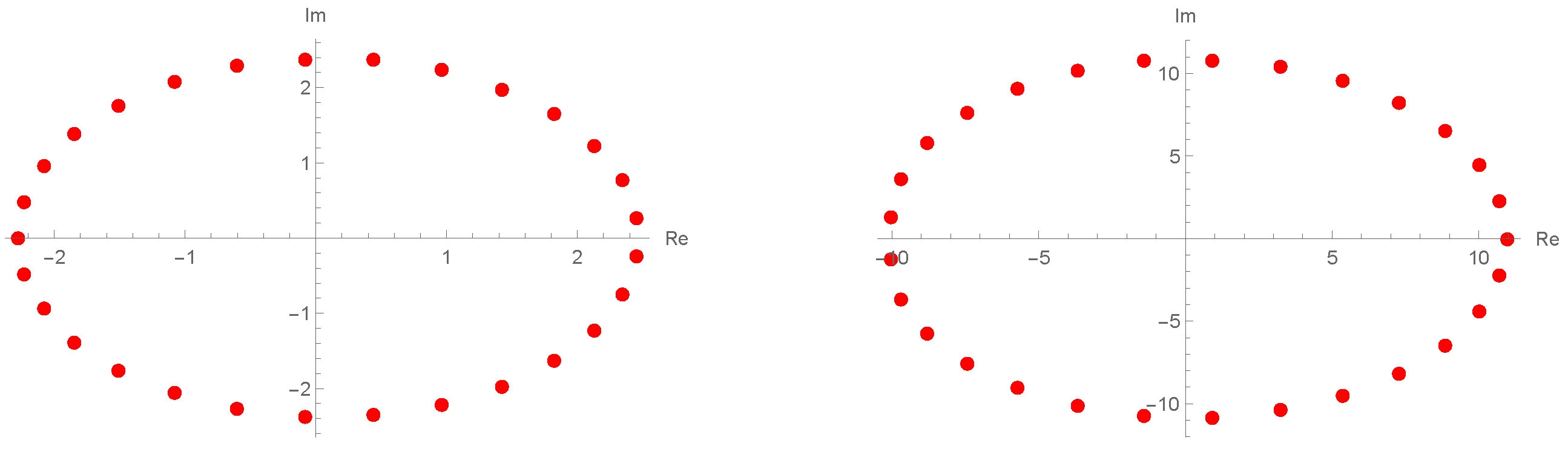
Figure 1 shows the structure of the approximate roots of $(\mathit{p},\mathit{q})$-cosine Euler polynomials. Given $\mathit{p}=0.5$, $\mathit{q}=0.9$, $\mathit{y}=5$, and $\mathit{n}=30$, we see that the structures of the approximate roots are as the left. Moreover, to determine the properties that depend on the value of p, we can check the right graph of Figure 1 to figure out $\mathit{q},\mathit{y},\mathit{n}$ under the same circumstances as the left figure except when the value of p is changed to $\mathit{p}=0.1$.

In Figure 1, we can see that the values of the approximate roots becomes bigger as the values of p become smaller, and the two graphs show that the approximate roots are located in an elliptical form.

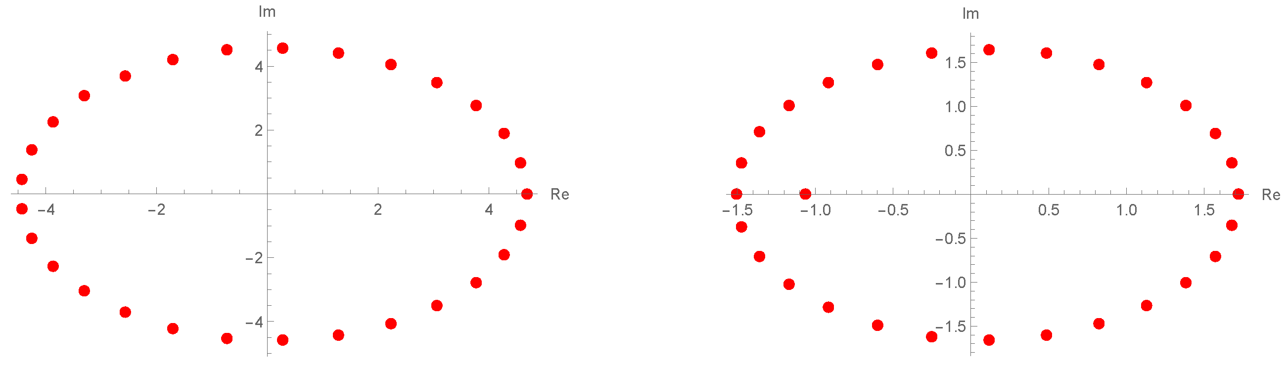
This time, let’s change the value of y to check the movement of the roots. The left side of Figure 2 is the location of the approximate roots obtained under conditions of $\mathit{p}=0.5$, $\mathit{q}=0.9$, and $\mathit{y}=10$, and the right side of the figure is the structure of the approximate roots that appears when $\mathit{y}=3$ under conditions such as the left side.

In Figure 2, its natural to compare with the left graph in Figure 1. As the value of y gets bigger, so does the approximations of the roots, and as the value of y decreases, so does the approximations of the roots.

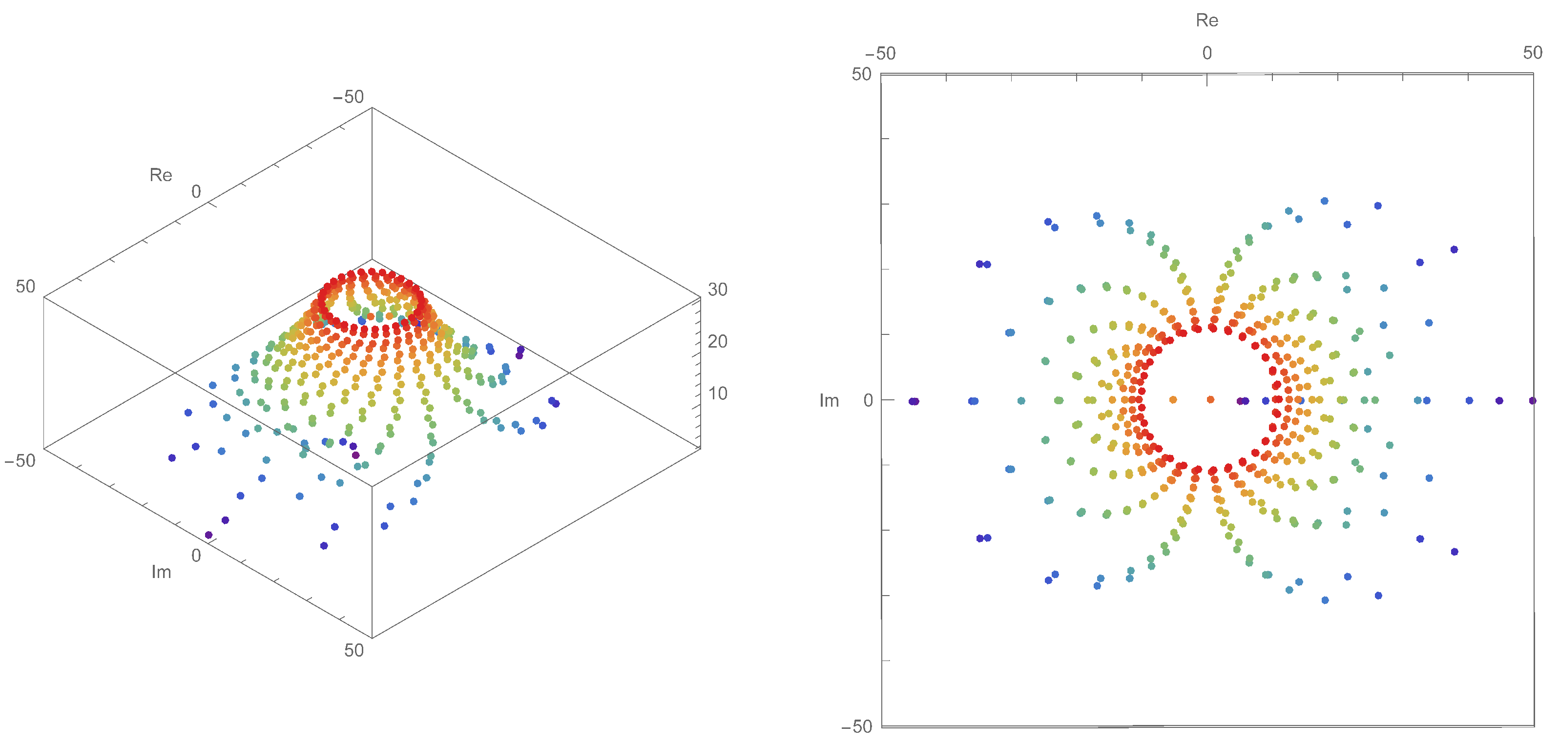
The following Figure 3 shows a stacking structure of approximate roots that appears when $\mathit{p}=0.1$, $\mathit{q}=0.9$, and $\mathit{y}=5$ are conditioned on $(\mathit{p},\mathit{q})$-cosine Euler polynomials and when the value of n varies from 1 to 30. In Figure 3, the smaller the value of n in $(\mathit{p},\mathit{q})$-cosine Euler polynomials, the wider the position of approximation roots, and the bigger the value of n, the more specific the approximation roots appear to be. Here, the red dots shown in Figure 3 are the positions of approximate roots of $(\mathit{p},\mathit{q})$-cosine Euler polynomials when n has a value of 30.

Here, we can see through Figure 1, Figure 2 and Figure 3 that the structure of the approximate roots appears approximately circular in shape. Furthermore, even when $\mathit{p}=0.9,\mathit{q}=0.1$, and $\mathit{y}=5$, we can confirm that the larger the value of n gets, the closer the approximation values are to a circle form. When we check these forms of plots, we can guess that approximate roots exist in a form of circles may exist as the value of n grows.

To confirm the above idea, we look for approximations of the roots of ${}_{\mathit{C}}{\mathcal{E}}_{\mathit{n},\mathit{p},\mathit{q}}(\mathit{x},\mathit{y})$. The following table shows approximations of the roots of $(\mathit{p},\mathit{q})$-cosine Euler polynomials which appear when $\mathit{n}=50$, $\mathit{p}=0.5$, $\mathit{q}=0.9$, and $\mathit{y}=5$.

From Table 1 above, we can find Figure 4 as follows.

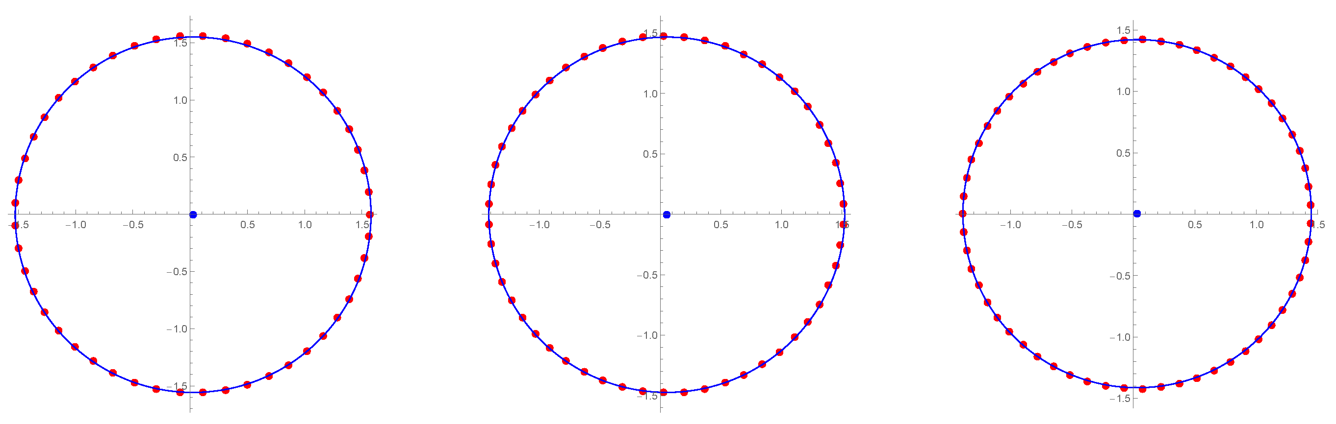
In Figure 4, we can grasp the interesting features of approximate roots of $(\mathit{p},\mathit{q})$-cosine Euler polynomials. As n grows larger, we see that the position of approximations has a shape close to a circle. In Figure 4, we plot the approximation circle in blue when $\mathit{n}=50$ on the left, $\mathit{n}=55$ in the middle, and $\mathit{n}=60$ on the right. The center of each circle is also marked by a blue dot. The center, radius, and error range of the circle represented in Figure 4 are found as shown in Table 2. The circle equation of approximate roots for ${}_{\mathit{C}}{\mathcal{E}}_{50,0.5,0.9}(\mathit{x},5)$ is ${(\mathit{x}-0.0246014)}^2+{(\mathit{y}-4.85622\times {10}^{-13})}^2=1.55359$, the circle equation of approximate roots of ${}_{\mathit{C}}{\mathcal{E}}_{55,0.5,0.9}(\mathit{x},5)$ is ${(\mathit{x}-0.0505825)}^2+{(\mathit{y}+7.41793\times {10}^{-9})}^2=1.46969$, and the circle equation of approximate roots of ${}_{\mathit{C}}{\mathcal{E}}_{60,0.5,0.9}(\mathit{x},5)$ is ${(\mathit{x}-0.0324048)}^2+{(\mathit{y}-3.1025\times {10}^{-9})}^2=1.41776$.

As it can be seen in Table 2, we can see that as n becomes larger, the radius becomes smaller. It can also be seen that the margin of error is reduced. Here, we find in Figure 2 that roots exist on the real axis when $\mathit{n}=30$ and $\mathit{y}=3$. The value of this point is $-1.04899$ and we have found the equation of the circle closest to the approximate roots except for these points. This can also be seen when $\mathit{n}=40$. These experiments suggest that the form of approximate roots in the higher order polynomials of ${}_{\mathit{C}}{\mathcal{E}}_{\mathit{n},0.5,0.9}(\mathit{x},5)$ will conform to a circular form, and that the center of the circle will exist close to the origin.

4. Conclusions

In this paper, we looked for various properties of $(\mathit{p},\mathit{q})$-cosine Euler polynomials. Based on these contents, we were able to determine the positions of approximation roots that appear differently depending on the values of p, q and y, as well as the equations associated with approximation roots. Depending on the values of p, q and y, the value of approximation roots varies, but as n increases, it is assumed that the stacking structure for each approximation root will become almost circular, and we can find a shape with a small error for the approximation roots. The effort to generalize the position and stacking structure of approximate roots of these higher-order equations is considered a challenge to be solved in the future.