Article

Modeling and Optimization for Multi-Objective Nonidentical Parallel Machining Line Scheduling with a Jumping Process Operation Constraint

1
School of Mechanical Science and Engineering, Huazhong University of Science and Technology, Wuhan 430074, China
2
School of Mechanical and Electrical Engineering, Guangzhou University, Guangzhou 510000, China
3
College of Mechanical and Electronic Engineering, Wenzhou University, Wenzhou 325000, China
*
Author to whom correspondence should be addressed.
Symmetry 2021, 13(8), 1521; https://doi.org/10.3390/sym13081521
Submission received: 13 July 2021 / Revised: 11 August 2021 / Accepted: 13 August 2021 / Published: 18 August 2021
(This article belongs to the Special Issue Theoretical Computer Science and Discrete Mathematics)

Abstract

:
This paper investigates the nonidentical parallel production line scheduling problem derived from an axle housing machining workshop of an axle manufacturer. The characteristics of axle housing machining lines are analyzed, and a nonidentical parallel line scheduling model with a jumping process operation (NPPLS-JP), which considers mixed model production, machine eligibility constraints, and fuzzy due dates, is established so as to minimize the makespan and earliness/tardiness penalty cost. While the physical structures of the parallel lines in the NPPLS-JP model are symmetric, the production capacities and process capabilities are asymmetric for different models. Different from the general parallel line scheduling problem, NPPLS-JP allows for a job to transfer to another production line to complete the subsequent operations (i.e., jumping process operations), and the transfer is unidirectional. The significance of the NPPLS-JP model is that it meets the demands of multivariety mixed model production and makes full use of the capacities of parallel production lines. Aiming to solve the NPPLS-JP problem, we propose a hybrid algorithm named the multi-objective grey wolf optimizer based on decomposition (MOGWO/D). This new algorithm combines the GWO with the multi-objective evolutionary algorithm based on decomposition (MOEA/D) to balance the exploration and exploitation abilities of the original MOEA/D. Furthermore, coding and decoding rules are developed according to the features of the NPPLS-JP problem. To evaluate the effectiveness of the proposed MOGWO/D algorithm, a set of instances with different job scales, job types, and production scenarios is designed, and the results are compared with those of three other famous multi-objective optimization algorithms. The experimental results show that the proposed MOGWO/D algorithm exhibits superiority in most instances.

1. Introduction

Flow shop scheduling problems are the most common and widely studied problems in the manufacturing industry, and the examined problems are usually simplified versions of the real flow shop scheduling problem so as to reduce the difficulty of modeling and solving these problems. These oversimplified schemes often cannot perfectly solve such scheduling problems in the actual environment. In real-world manufacturing situations, some special constraints or uncertainties must usually be considered and handled, such as sequence-dependent setup times [1,2,3], the kinds of parallel machines under study [4,5], machine eligibility constraints [6,7,8,9], resource constraints [10,11], and fuzzy stochastic demand [12,13]. Considerations of these additional constraints and uncertainties make the developed scheduling models closer to real production scenarios, but also increase their scheduling complexity. Because of product iteration requirements and the diversified needs of customers, production systems must often address multivariety production on multiple production lines. This is very common in manufacturing enterprises such as those in the automobile industry and household appliance industry, as well as for construction machinery manufacturers. When coping with these situations, the equipment configurations of multiple lines may be different for meeting multivariety production. In this paper, we study this nonidentical parallel production line scheduling problem. To improve the machine utilization and shorten the waiting times of the jobs to be processed, a jumping process operation is often used. This means that if a certain process operation of a job is finished, it can move to another production line to complete the subsequent process operations. This jumping process operation is unidirectional. To solve this kind of scheduling problem, nonidentical parallel line scheduling with a jumping process operation (NPPLS-JP) is proposed; this is also in essence a parallel production line scheduling problem. Notably, the proposed NPPLS-JP problem is an NP-hard problem because of its complexity.
This NPPLS-JP problem is derived from the axle housing machining workshop of an axle manufacturer. Axle housing is an important part of axle production; it usually adopts make-to-stock (MTS) production and make-to-order (MTO) assembly. The machining of an axle housing is shown in Figure 1. The axle manufacturer adopts nonidentical parallel production lines for axle housing machining. There are two parallel production lines (A and B) in the axle housing machining workshop, and each production line is installed linearly, as shown in Figure 1. The physical structures of the two production lines are symmetrical. Each production line contains five stages corresponding to five operations, and the parallel machines at any stage of each line are identical. The corresponding stages of production lines A and B have similar functions, but the configurations of the machines in the different lines are different in order to meet the needs of multivariety mixed production. In this production situation, the production load of each stage on any line is not easy to balance via a simple scheduling scheme.
According to the different vehicle models, there are eight types of axle housing products that can be processed on line A and line B with multivariety mixed model production; all types of products are processed through five operations, as shown in Figure 1. Two types of axle housing products have machine eligibility constraints, and the operation “combined machining I” can only be performed at the corresponding machines in production line B; the others can finish processing on any line independently. For different types of axle housing, the different processing times required for the same operation on the same machine and the different mixing ratios of the various axle housing types increase the complexity of the scheduling problems. It is difficult to balance all the stages of each production line, so a jumping process operation is adopted to address this problem by allowing a job to be processed on two production lines. For example, when the operation “combined machining I” is finished on line A, the job is transferred to line B to complete the subsequent machining operations; this is called the jumping process operation, and the stage “combined machining I” is called the jumping process point. A jumping process operation is unidirectional, which means that the axle housings processed on line A are allowed to be transferred to production line B, but not the other way around. Appropriate jumping process operations can reduce waiting times, improve the utilization rate of equipment, balance the production capacity of each stage, and ensure the due date of each order.
From the above description of a production system, it can be seen that the axle housing machining line scheduling problem has the following characteristics: (1) The configurations of the multiple production lines are similar but not the same. (2) Mixed multivariety production is adopted to organize production. (3) Several jobs with special types have machine eligibility constraints. (4) The jumping process operation is unidirectional in the production process. This problem can be regarded as a variant and extension of the flow shop scheduling problem or general parallel production line scheduling problems, and it involves four key decision-making processes, namely: job sequencing decisions, parallel line decisions, parallel machine decisions, and job jumping process operation decisions. It is obvious that the NPPLS-JP problem proposed in this paper is a rather complex scheduling optimization problem.
Because of the fierce competition in the market and the diversified needs of customers, the NPPLS-JP problem is widespread in manufacturing environments and has an important impact on the manufacturing efficiency of production systems. However, there is no relevant research on this topic in the existing literature, so the study in this paper is of exploratory and practical significance. In this paper, we establish a scheduling model for the NPPLS-JP problem, which involves multivariety mixed model production, multiline scheduling, and machine eligibility constraints. The objectives are to minimize the makespan and earliness/tardiness penalty in a production cycle. In the NPPLS-JP model, to more closely approximate the actual production environment, the due date of a production order denoted by the fuzzy earliness/tardiness penalty model [14], and a hybrid algorithm combining the grey wolf optimization algorithm and the multi-objective evolutionary algorithm based on decomposition (MOEA/D) are proposed to solve the NPPLS-JP problem.
The remainder of this paper is organized as follows. Section 2 reviews the literature relevant to multivariety mixed model production, parallel line scheduling, and multi-objective optimization. Section 3 gives a general statement of the NPPLS-JP problem and establishes a production-based, order-oriented, multi-objective scheduling model. Section 4 proposes the multi-objective grey wolf optimizer based on decomposition (MOGWO/D) for NPPLS-JP and describes the procedures in detail. Section 5 tests the performance of the proposed MOGWO/D algorithm by comparing it with three other famous multi-objective algorithms based on a set of designed test instances, and the experimental results are analyzed. Section 6 summarizes the research content and discusses the direction of future research.

2. Literature Review

Mixed model production refers to the production of a variety of products on a single production line to increase the flexibility of the line and meet the multivariety and small-batch production demands. For multiproduct demands, mixed model production is widely adopted by manufacturing enterprises, especially in assembly workshops [15,16]. Because of the widespread application of mixed model production, many scholars are devoted to research in this field and have made many achievements [17,18,19,20,21].
Mcmullen et al. [22] studied the mixed model scheduling problem with the consideration of a setup time. They presented a bean search heuristic method to obtain an efficient front. Leu and Hwang [23] proposed a resource-constrained mixed-production flow shop scheduling system for mixed precast production task problems and developed a search method based on a genetic algorithm (GA) to minimize the output makespan under resource constraints and mixed production. Wang et al. [24] studied final assembly line scheduling, which considers order scheduling and mixed model sequencing simultaneously, and combined the original artificial bee colony (ABC) algorithm with some steps of the GA and Pareto optimality to solve this problem. Bahman et al. [25] constructed a mixed-integer linear programming model with a tighter linear relaxation for a realistic automotive industry assembly line, including a set of specific requirements involving moving workers and limited workspace. Alghazi and Kurz [26] proposed a mixed model line-balancing integer program for mixed model assembly lines with the aim of minimizing the number of chemical workers; a constraint programming model was established to address larger assembly line balancing problems.
Parallel line scheduling problems are very common in both mass production and multiproduct production. Parallel line production can enhance the stability and flexibility of the production system and improve production efficiency. When one production line breaks down, not all production activities are stopped. All parallel lines may have the same number of processing stages, the pieces of equipment in the same stage are similar and can complete the same production processes, and every line can substitute for all other lines to produce all or some types of the desired products [27]. However, in some situations, the configurations of the machines in different lines are nonidentical; this situation is more convenient for the production of multiple products. For example, two types of equipment in different production lines can independently complete the operation of milling surfaces, but the machining accuracies are different.
Haq et al. [28] studied the line scheduling problem with multiple parallel processing in job shops. Each job can only be processed on a particular line and is not allowed to move between parallel lines. Meyr and Mann et al. [29] introduced a new solution approach to determine the lot-sizing and scheduling problem for parallel production lines with the consideration of scarce capacity; sequence-dependent setup times; and the deterministic, dynamic demands of multiple products. Mumtaz et al. [30] investigated the multiple assembly line scheduling problem for a printed circuit board (PCB) assembly and developed a hybrid spider monkey optimization approach with an improved replacement strategy to solve it. Rajeswari et al. [27] presented parallel flow line scheduling with a dual objective to minimize the tardiness and earliness of jobs. All parallel flow lines had similar sets, and the authors developed a hybrid algorithm that used a GA and particle swarm optimization (PSO) to incorporate greedy randomized adaptive search to address the problem. Ebrahimipour et al. [31] proposed linear programming and a bagged binary knapsack to address the multiple production line scheduling problem. Mumtaz et al. [32] developed a mixed-integer programming model for the multilevel planning and scheduling problem of parallel PCB assembly lines, and a hybrid spider monkey optimization (HSMO) algorithm was proposed.
Multi-objective optimization refers to a situation where more than one conflicting objective is to be optimized simultaneously. It is often impossible to obtain an optimal solution as in a single-objective optimization problem, but a set of tradeoff solutions, namely, nondominated solutions, can be used to choose the most suitable solution according to the actual requirements. Therefore, it is more applicable to the actual situation, which requires the consideration of multiple indicators affecting decision making. As it is conducive to obtaining an ideal decision making effect, multi-objective optimization has a wider application field and more practical value. MOEAs are global optimization algorithms based on populations that simulate the evolution process of natural organisms. Since the whole solution set can be obtained in one run, MOEAs have become some of the mainstream algorithms in multi-objective optimization. According to their selection mechanisms, MOEAs can be classified into three classes [33]: Pareto-based algorithms, indicator-based algorithms, and decomposition-based algorithms. The Pareto-based method was first proposed by Goldberg et al. [34] and has been widely studied since then. Many classical multi-objective optimization algorithms are based on the Pareto relation, and many have been proposed based on the Pareto dominance relationship, such as the famous SPEA [35], SPEA2 [36], and NSGA-II [37]. The indicator-based method uses performance evaluation indicators to guide the search process and the choice of solutions [38,39]. The MOEA/D was first proposed by Zhang and Hui in 2007 [40], and it is the most representative multi-objective optimization algorithm based on decomposition. Different from the classical multi-objective optimization algorithms, it decomposes an input multi-objective optimization problem (MOP) into a series of single-objective optimization subproblems by using a set of uniformly distributed weight vectors and optimizing these subproblems simultaneously. Since the MOEA/D was proposed, it has attracted increasing attention from scholars, improvements and applications for the MOEA/D are constantly emerging, and it has become one of the best multi-objective optimization algorithms.
Li and Landa-Silva et al. [41] proposed evolutionary multi-objective simulated annealing (EMOSA), which incorporates a simulated annealing algorithm and introduces an adaptive search strategy. The experimental results showed that the algorithm obtained a good effect in terms of solving the multi-objective knapsack problem and multi-objective salesman problem. Tan et al. [42] developed a multi-objective meme algorithm based on decomposition, which integrates a simplified quadratic approximation (SQA) into the MOEA/D as a local search operator to balance its local and global search strategies. Wang et al. [43] designed a multi-objective particle swarm optimization algorithm based on decomposition (MPSO/D). This algorithm adopts relevant measures to ensure that only one solution is present in each subregion in oder to maintain solution diversity, and the fitness is calculated by the crowding distance. Ke and Zhang et al. [44] proposed the MOEA/D-ACO algorithm, which incorporates ant colony optimization (ACO) into the MOEA/D; they then tested the performance of the proposed algorithm in 12 instances and obtained good results. Alhindi et al. [45] developed a hybrid algorithm called MOEA/D-GLS, which integrated guided local search (GLS) with the MOEA/D to promote the exploitation ability of the original MOEA/D. The experimental results showed that the proposed MOEA/D-GLS was superior to the original MOEA/D. Zhang et al. [46] proposed MOEA/D-EGO to address expensive MOPs. In this method, the input problem is decomposed into several subproblems, and a prediction model is established for each subproblem based on the evaluated points in order to reduce modeling costs and improve the prediction quality. Wang et al. [47] proposed adaptive replacement strategies by adjusting the problem size dynamically for the MOEA/D. This approach can balance the diversity and convergence of the MOEA/D.
However, according to the no free lunch theorem [48], no algorithm can solve all of the optimization problems in all of the fields. Because of the continuous emergence of new optimization problems, the existing algorithms cannot solve these new optimization problems well, so new algorithms or improved algorithms are needed. The MOEA/D algorithm exhibits good diversity in solving MOPs; its characteristics include simplicity, few parameters, and better result distributions. In this paper, the MOGWO/D, which incorporates the GWO into the MOEA/D, is proposed to solve the NPPLS-JP problem.

3. Problem Description and Mathematical Modeling

3.1. Problem Definition and Assumption

Suppose that O orders are processed in L production lines, the job types for each order are the same and those for different orders may be different, and the operations of each type of job are predetermined and similar. All production lines have the same number of stages, and the machine configurations may be different. If parallel machines exist in some stages of the production line, they are identical parallel machines. Some types of jobs may have machine eligibility constraints, namely some job operations must be carried out on specific machines at certain stages of some production lines. For any production line l , if s is set as the jumping process operation point, it means that after processing is completed in stage s , the job can be transferred to line l to continue the processing of the subsequent operations ( l l   a n d   l , l { 1 , 2 , , L } ); the jumping process operation is unidirectional. The scheduling objectives are to minimize the makespan and the earliness/tardiness penalty cost.
In addition, there are usually several complicated constraints and perturbations in the real-world production environment. To prevent the loss of generality and reduce the computational complexity of the scheduling model, some modeling assumptions are given, as follows.
(1)
The type, quantity, and due date of each order are known.
(2)
The jobs in each order are of the same type.
(3)
All the machines in the production system are available at the beginning.
(4)
The processing times and setup times of the jobs on each machine do not overlap.
(5)
Each job can be processed on only one machine at any time, each machine can process only one job at any time, and operations cannot be interrupted.
(6)
For each job, the jumping operation can only occur once.
(7)
The jumping process operation point is singular, fixed, and unidirectional.
(8)
The setup time and machine breakdown time are ignored.
Meanwhile, to solve the NPPLS-JP problem more conveniently, the concept of a virtual production line is introduced. This means that if there is a jumping process operation point in the manufacturing process of a job of a certain type, all the stages in two different production lines that can complete the processing of jobs of this type are regarded as a new production line, namely, a virtual production line.
In a real-world production environment, a breach of the order due dates is not always unacceptable. In general, a few occurrences of tardiness are allowed, to achieve the smallest due date penalty cost across the total orders. Here, the fuzzy due date is used to deal with this situation. Trapezoidal fuzzy due date and triangular fuzzy due date are two common fuzzy due dates that have been investigated in the literature regarding scheduling problems [14,49,50,51]. Most researchers choose the type of fuzzy due date depending on the research background and problem characteristics. In our research, neither early nor late completion were the best solutions for the automobile industries. Completing the production order in advance will increase the inventory cost, while the order delay will lead to customer penalty loss. Finishing and delivering the orders in a given period is the most feasible result. Therefore, the trapezoidal fuzzy due date and earliness/tardiness penalty cost model was adopted in this scheduling problem according to the real-world production requirement.
As shown in Figure 2a–b, (a) is the trapezoidal fuzzy due date and earliness/tardiness penalty cost model, (b) is the corresponding satisfaction model of the fuzzy due date. Model (a) shows each order has a corresponding trapezoidal fuzzy due date that is denoted by a trapezoidal fuzzy number d o = ( d o 1 , d o 2 , d o 3 , d o 4 ) , and the earliness/tardiness penalty cost coefficients are α o and β o , respectively. A completion time before d o 1 it means that the orders are produced prematurely, and additional inventory costs are generated; if the completion time comes after d o 4 , the production order seriously violates the due date requirement. These two cases are both unacceptable, so the satisfaction is 0, and the maximal earliness/tardiness penalty is imposed. If the completion time is in the time interval [ d o 1 , d o 2 ] or [ d o 3 , d o 4 ] , the due date penalty costs decrease and increase linearly, respectively, and the corresponding due date satisfaction is just the opposite. Only in the time interval [ d o 2 ,   d o 3 ] are the completion times reasonable, and the due date penalty cost in this case is 0. Therefore, the production orders should be arranged optimally in terms of time according to different due dates and earliness/tardiness penalty costs.

3.2. Mathematical Modeling

A mathematical model for the proposed NPPLS-JP problem is established using the above notations, and the two objective functions, which minimize the makespan and earliness/tardiness penalty cost, are formulated as Equations (1) and (2), respectively.
M i n f 1 = max { C o }  
M i n f 2 = o = 1 O P o
where the calculation formulas of the completion time and due earliness/tardiness penalty for order o are formulated as Equations (3) and (4), respectively:
C o = max { u i , o C i }   i J
P o = {   α o C o < d o 1 α o · d o 2 C o d o 2 d o 1 d o 1 C o < d o 2 0 d o 2 C o d o 3 o O   β o · C o d o 3 d o 4 d o 3 d o 3 C o < d o 4   β o C o d o 4
The constraints are as follows:
l = 1 L s = 1 ( s l 1 ) ( X i , s , l Y i , s , s ) = 1   i J ;   s = ( s + 1 )
l = 1 L s = ( s l + 1 ) ( S 1 ) ( X i , s , l Y i , s , s ) = 1   i J ;   s = ( s + 1 )
Y i , s l , ( s l + 1 ) = 0 , 1   i J
l = 1 L ( X i , s , l X i , s , l ) = X i , s , s   i J ;   s { 1 , 2 , , ( S 1 ) } ;   s = ( s + 1 )
k = 1 M s l X k , i , s , l = X i , s , l   i J ;   s S ;   l L
X i , s , l o = 1 O t = 1 N t l = 1 L x i , o x o , t x t , s , l   i J ;   s S ;   l L
l = 1 L k = 1 M s l X k , i , s , l = 1   i J ;   s S
Z k , i , i , s , l + Z k , i , i , s , l X k , s , i , l   i , i J ;   i i ;   s S ;   k M s , l ;   l L
C k , s , i , l X k , s , i , l + M ( 1 Z k , i , i , s , l ) C k , s , i , l X k , s , i , l + o = 1 O t = 1 N t ( p t t , k , s x o , t x i , o ) X k , s , i , l i , i J ;   i i ;   s S ;   k { M s , l M s , l } ;   l , l L
C k , s , i , l X k , s , i , l + M ( 1 X k , s , i , l ) C k , s , i , l X k , s , i , l + o = 1 O t = 1 N t ( p t t , k , s x o , t x i , o ) X k , s , i , l s { 1 , 2 , , S 1 } ;   s = ( s + 1 ) ;   k M s , l ;   k M s , l ;   l , l L
Among the above constraints, constraints (5)–(7) together define the jumping process operation. Constraint (5) defines the operations before the jumping process operation point (including the operation on the jumping process operation stage), which can only be completed in one production line. Constraint (6) restricts all of the operations after the jumping process operation point for each job that can only be processed on the same production line. Constraint (7) states the jumping process operation for any job may or may not occur after completing another jumping process operation, and the three constraints together guarantee that the jumping process operation can only occur once at most. Constraint sets (8) and (9) define the relationships between several decision variables. Constraint (10) states that the processing of each job operation must satisfy the machine eligibility constraints. Constraint (11) ensures that each operation of a job can only be processed on one machine. Constraint sets (12) and (13) together restrict the processing sequence of two jobs on a machine to only one possible result. Constraint (14) guarantees that one machine can only process one job at a time, which means that the completion time of the current job is longer than the sum of the completion time of the immediate predecessor job and the processing time of the current job. Constraint (15) ensures that a job is processed by only one machine at a time, that is, the completion time of the job operation is greater than the sum of the completion time of the immediate predecessor operation and the processing time of the current operation.

4. Proposed MOGWO/D Algorithm

The MOEA/D provides a general framework that allows any single objective to be applied to the subproblems of a MOP [41]. Compared with the other multi-objective optimization algorithms, such as the Pareto-based optimization algorithms, MOEA/D has less computational complexity, and its results have better diversity. In this section, we present a hybrid algorithm that combines GWO with MOEA/D, and uses the mechanism of searching for prey in the GWO algorithm to enforce a balance between exploration and exploitation. According to the characteristics of the NPPLS-JP problem, problem-specific encoding and decoding rules are given, and some main procedures in the proposed MOGWO/D are also stated in detail.

4.1. Original GWO

The GWO was inspired by the leadership hierarchy and hunting behaviors of grey wolves [52]. In GWO, initial populations are used to simulate the grey wolf group, which is divided into four hierarchies; the solutions with the best, second, and third fitness values are α, β, and δ, respectively, are utilized to find the optimal solution by simulating the hunting process of grey wolves. In the process of hunting, the location of the prey is unknown. Therefore, to simulate the hunting behavior of grey wolves and the prey behavior from the perspective of mathematical modeling, suppose that α ,   β , and δ are closest to the potential position of the prey. Under the guidance of α ,   β , and δ , the position vector is updated to approximate the optimal solutions in the search space.
The main procedure of wolf hunting includes encircling prey and hunting, and the mathematical models for grey wolves approaching and encircling their prey are as follows:
D = | C X p ( t ) X ( t ) |
X ( t + 1 ) = X p ( t ) A D
A = 2 a r 1 a
C = 2 r 2
In Equations (16) and (17), X p indicates the position vector of the prey and X is the position vector of the grey wolf. A and C are coefficient vectors, and the calculation methods are shown in Equations (18) and (19). By changing the value of the vector A , the search process can be guided. When | A | > 1 , α, β, and δ diverge from each other, which is good for global search; when | A | < 1 , α, β, and δ converge to the prey, which contributes to the local search. The parameter C is generated randomly to help grey wolves jump out of the local optima.
In Equations (18) and (19), r 1 and r 2 are randomly generated in [ 0 ,   1 ] , and the values of the parameter a linearly decrease from 2 to 0 over the course of the iterations. During the process of hunting, the position vectors are updated using the following equations:
X 1 = X α A 1 | C 1 X α X |
X 2 = X β A 2 | C 2 X β X |
X 3 = X δ A 3 | C 3 X δ X |
X ( t + 1 ) = X 1 + X 2 + X 3 3
In Equations (20)–(23), X α ,   X β , and X δ are the position vectors of α, β, and δ, respectively, and X denotes the current position vector that needs to be updated.

4.2. MOGWO/D Algorithm Framework

The proposed MOGWO/D is a hybrid algorithm that integrates GWO into MOEA/D. Similar to the original MOEA/D, the MOGWO/D algorithm decomposes the input multi-objective problem into a series of single-objective scalar optimization subproblems by utilizing a set of uniformly distributed weight vectors and a scalar function. Here, we use the Tchebycheff method to construct each subproblem; then, subproblem i can be described as follows [40]:
M i n i m i z e   g t e ( x | λ i , z * ) = max 1 j m { λ i j | f i ( x ) z m * | }
where z i * is the i -th component of reference point ( z 1 * ,   z 2 * ,   ,   z m * ) T ,   z i * = min { f i ( x ) | x Ω } ,   i = 1 ,   2 ,   ,   m ,   λ i = ( λ i 1 ,   λ i 2 ,   ,   λ i m ) T . The purpose is to minimize each single-objective function g t e ( x i | λ i ,   z * ) , and each subproblem uses the approach of the GWO to update its position vectors. It is worth noting that finding accurate reference points is difficult and time-consuming work, so the best objective values z = ( z 1 ,   z 2 ,   ,   z m ) T method is used in the initial population as the initial reference point, and to update the reference point over the course of iterations by generations.
As the normalization method for objectives is conducive to increase the uniformness of the obtained solutions when the input objectives are disparately scaled [40], we used a simple normalization method to replace f i and obtained a normalization Tchebycheff approach, as follows.
M i n i m i z e   g t e ( x | λ i , z ) = max 1 j m { λ i j | f i ( x ) z i * z i n a d z i * | }
where z * is the reference point and z n a d = { z 1 n a d , z 2 n a d , , z m n a d } is the nadir point in the objective space. In our calculation, z * is replaced by z in Step 2.3 of Algorithm 1, and the maximum value of f i ( x ) in the current population is the substitute for z i n a d . This calculation strategy can meet the needs of the algorithm.
Algorithm 1 MOGWO/D
  Input:
  A multiobjective problem;
  A stopping criterion;
  A set of uniformly spread weight vectors { λ 1 ,   λ 2 ,   ,   λ N } ;
   N : population size (equal to the number of the weight vectors or subproblems);
   T : neighborhood size;
   T : the number of position vectors in the neighborhood to be updated of a subproblem (where T < T ).
Output:
  External population, EP for short.
Step 1) Initialization:
  Step 1.1) Set EP = ∅;
  Step 1.2) Generate a set of uniformly distributed weight vectors { λ 1 ,   λ 2 ,   ,   λ N } , calculate the Euclidean distances of any pair of weight vectors, for i = 1 ,   2 ,   ,   N ,   defines   a   set   B ( i ) = { i 1 ,   i 2 ,   ,   i T } ,   λ i 1 ,   λ i 2 ,   ,   λ i T are T closest weight vectors of the weight vecto λi.
  Step 1.3) Randomly generate an initial population { x 1 ,   x 2 ,   ,   x N } or use a problem-specific approach. The objective of each position vector is calculated and labeled as F V i ,   F V i = F ( x i ) ,   i = 1 ,   2 ,   ,   N .
  Step 1.4) Initialize z = ( z 1 ,   z 2 ,   ,   z m ) T ,   z i = m i n { f i ( x 1 ) ,   f i ( x 2 ) ,   ,   f i ( x N ) } ,   i = 1 ,   2 ,   m .
  Step 1.5) Calculate g t e ( x j | λ i ,   z * ) for each j B ( i ) , and the three best position vectors are labeled as x α ,   x β and x δ , respectively corresponding to weight vector λ i .
Step 2) Update:
  for i = 1, 2, ⋯,N, do
  Step 2.1) Randomly select T indexes k 1 , k 2 , ,   k T   from   B ( i ) , then yield a set of new position vectors x k 1 , x k 2 , , x k T according to the Equations (20)–(23) by the guidance of x α i x β i ,   and   x δ i ,   set   P S ( i ) = { x k 1 , x k 2 , , x k T } .
  Step 2.2) Update of x α i ,   x β i   and   x δ i . Comparing the value of g t e ( x | λ i ,   z ) with g t e ( x α i | λ i ,   z ) ,   g t e ( x β i | λ i ,   z ) and g t e ( x δ i | λ i ,   z ) ,   x P S ( i ) , then update x α i ,   x β i   and   x δ i with the three best position vectors of all.
  Step 2.3) Update of z. For each j = 1, 2, ⋯, m, if f j ( x α i ) < z j ,   set   z j = f j ( x α i ) .
  Step 2.4) Update of neighborhood. For each j B ( i ) ,   if   ( x α i ,   | λ j ,   z ) } g t e ( x j | λ j ,   z ) ,   set   x j = x α i ,     and   update   of   F V j = f ( x α i ) .
  Step 2.5) Update of EP. Add f ( x α i ) to EP if no vectors in EP dominate f ( x α i ) ; if the number of vectors exceeds the EP capacity, the kth nearest neighbor method is used as a truncation strategy. If the vectors in EP are dominated by f ( x α i ) , remove from EP.
Step 3) Stopping criterion:
If the stopping criteria is satisfied, stop running and output EP. Otherwise, return to Step 2.
Similar to the original MOEA/D, the MOGWO/D algorithm (Algorithm 1) also optimizes a number of scalar optimization subproblems simultaneously in one iteration, thus improving the optimization efficiency of the proposed algorithm.

4.3. Generate a Set of Uniform Weight Vectors

In Step 1.2 of Algorithm 1, a simplex-lattice design [53] is adopted to generate a set of uniformly distributed weight vectors λ i = ( λ 1 i ,   λ 2 i ,   ,   λ m i ) ,   i N , and m is the dimensionality of the objective space. For each λ i , j = 1 m λ j i =1, and λ j i { 0 ,   1 H ,   2 H ,   ,   H H } , H is a predetermined positive integer determined according to the sizes of the problems, so, a total of C H + m 1 m 1 weight vectors are obtained. For each λ i , the Euclidean distance to any weight vector is calculated, defining a set B ( i ) = { i 1 ,   i 2 ,   ,   i T } , in which λ i 1 ,   λ i 2 ,   ,   λ i T are the indexes of the T closest weight vectors to λ i ; then, B ( i ) is called neighborhood of λ i (including λ i itself, as λ i is the closest weight vector to itself, of which the Euclidean distance is 0). At the same time, the response of x i to λ i also generates a neighborhood, and each individual in the neighborhood corresponds to each weight vector determined by B ( i ) .

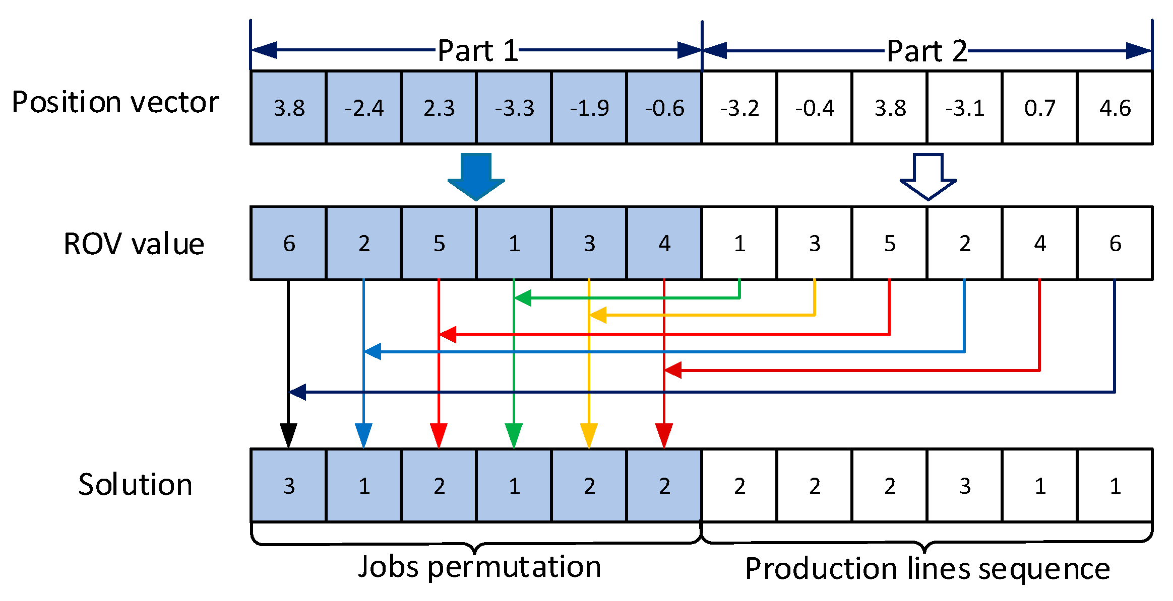
4.4. Encoding and Decoding

In the proposed MOGWO/D algorithm, the encoding method is similar to the original GWO, and the initial population is randomly generated from a uniform distribution. All position vectors in the initial population are continuous, but the scheduling solutions to the proposed combinatorial optimization problem are not, so a decoding approach is needed to convert the continuous position vectors to the scheduling solutions.
In the proposed NPPLS-JP problem, each position vector needs to include two pieces of information, a job permutation and a production line sequence, and the production line sequence corresponds to the job permutation. Suppose that there are O orders in a planning cycle; if the number of jobs in the order o is N o , then there are a total of N = o = 1 O N o jobs in this planning cycle, and each position vector in the population is represented as x i = [ x 1 i ,   x 2 i ,   ,   x N i , | x ( N + 1 ) i ,   ,   x 2 N i ] . For convenience of expression, the first N position values are marked as Part 1, which corresponds to the job permutation, and the last N position values are marked as Part 2, which corresponds to the production line sequence.
Part 1 and Part 2 are decoded independently. The decoding methods for Part 1 and Part 2 are different because the machining operations of the jobs of some types have machine eligibility constraints. The selection of the production line involves the decoded information of Part 1, that is, the decoding process of Part 2 depends on the obtained jobs’ permutation. To discretize the continuous position vectors, the ranked-order value (ROV) rule [54] is used in the decoding processes of Part 1 and Part 2.
For each position value in Part 1 of the position vector, the ROV rule is used to generate ROVs according to the position values in ascending order. If identical position values exist, the ROVs increase from left to right, and then the ROV permutation is obtained. Then, the N 1 smallest values are picked and all are assigned a value of V 1 . V 1 is the order number of order 1, and N 1 is the size of order 1; similarly, ROVs ( N 1 + 1 ) to N 2 are picked and assigned V 2 . V 2 is the order number of order 2, and N 2 is the size of order 2. In the same way, the job permutation is obtained.
For Part 2, first, as in Part 1, the ROV sequence is obtained according to the position values in Part 2 in ascending order. The next step is different from Part 1. For each ROV in Part 2, the same ROV in Part 1 is found, the corresponding order number is obtained, and then its job type is determined. Then, the job type in the first column of the given line selection information table is found, and the corresponding number of optional lines in the second column is obtained. Next, the remainder of the current ROV divided by the number of available lines is obtained. Finally, the corresponding production line number in the third column is found according to the calculated remainder, and the production line number is assigned to the position in Part 2 corresponding to current ROV. In the same way, the production line sequence is obtained. This decoding method for Part 2 can prevent increases in the calculation cost due to invalid solutions caused by the selection of unusable production lines.
A simple example, as shown in Table 1, is used to demonstrate the decoding rules. The sizes of the three orders are two, three, and one, and the total number of jobs is 6six. The detailed decoding process for the example is shown in Figure 3.
In this example, there are a total of five jobs. Each position value of the position vector is taken from the uniform distribution U[−6, 6] so that the position vector x = [3.8, −2.4, 2.3, −3.3, −1.9, −0.6, −3.2, −0.4, 3.8, −3.1, 0.7, 4.6] can be obtained, where Part 1 is [3.8, −2.4, 2.3, −3.3, −1.9, −0.6], and Part 2 is [−3.2, −0.4, 3.8, −3.1, 0.7, 4.6]. For the decoding process, the production line selection information used in Part 2 is given in Table 2.

4.5. Updating the Position Vectors

The Tchebycheff approach is adopted to decompose the input MOP into N single-objective optimization subproblems and to optimize them simultaneously. The neighborhood of each subproblem is defined based on the distances between their weight vectors. Adjacent subproblems have similar approximate solutions, so each subproblem is optimized, and only the information of neighboring subproblems is used. For every generation, T position vectors corresponding to the subproblems are updated, where T is a positive integer smaller than the neighborhood size, and these T position vectors are randomly selected from the neighborhood corresponding to the subproblem.
Each selected position vector of each subproblem is updated, and this information is used in its neighborhood. First, position vectors are updated according to Equations (20)–(23) through the guidance of the current three best position vectors x α , x β , and x δ , and the position vector set P S = { x 1 , x 2 , , x T } of the subproblem is obtained. Second, calculating the g t e value of every position vector in the G S ( i ) = P S   { x α ,   x β , x δ } corresponding to λ i . Then, x α ,   x β , and x δ are updated with the best, second best, and third best position vectors in the GS(i) corresponding to the weight vector λ i , where x α is the optimal solution to the current subproblem. After that, the reference point is updated by calculating the objectives with x α ; if f j ( x α ) < z j , then z j = f j ( x α ) . Third, the neighborhood of the current subproblem is updated with respect to each position vector to the weight vectors of the neighborhood; for each j B ( i ) , if g t e ( x α | λ i ,   z * ) g t e ( x j | λ j ,   z * ) , x j = x α and F V j = f ( x α ) simultaneously. The pseudocode for implementing the update process in one iteration is shown in Algorithm 2.
Algorithm 2 The update process of one iteration
  While(stopping condition is not satisfied){
  //Main loop
  for(i = 1; iN; i++)
  {//optimize N subproblems simultaneously
  idxes = getRandoms(T, B(i));
  selectedPop = getIndividuals(neighborhood, idxes);
   PS ( i ) = updateIndividuls ( selectedPop ,   x α , x β ,   x δ ) ;
sortedPop = sort(PS(i));
x α = sortedPop ( 0 ) ;  
   x β = sortedPop ( 1 ) ;  
   x δ = sortedPop ( 2 ) ;  
   updateZ ( x α ) ;     //update the reference point;
   updateNeighborhood ( x α ) ;
   updateEP ( x α ) ;
    }
  }

4.6. Updating the External Population (EP)

After obtaining the best position vector x α of every subproblem in each generation, the EP needs to be updated. If the condition that F ( x α ) is not dominated by the individuals in the EP, F ( x α ) is added to the EP, and the individuals that are dominated by F ( x α ) are removed.
In the search process of the algorithm, excess individuals are added to the EP. Too many nondominated individuals are not of great significance for solving practical problems, but they increase the difficulty of the data analysis. Therefore, a special truncation strategy is used to maximize the retention of nondominated solution characteristics while maintaining the appropriate EP size. In this strategy, the k th nearest neighbor method [36] is used here to evaluate the individuals in the EP, and the calculation approach for the k th nearest neighbor distance is as follows.
D ( i ) = 1 σ i k + 2
k = | P | + | E P |
where D ( i ) is the inverse function of the Euclidean distance from individual i to its k -th nearest neighbor, which is used to reflect the density information of the objective space. σ i k is the k th nearest Euclidean distance of individual i , where the value of k is calculated using Equation (27), and | P | and | E P | are the population size and external population size, respectively. The smaller the D ( i ) value is, the more scattered the solutions are.

5. Computational Experiments and Results Analysis

NPPLS-JP is a novel multiline scheduling problem derived from a real-world manufacturing workshop; it is an extension of regular flow shop scheduling problems that has no related research. Therefore, there are no benchmarks available for the proposed MOGWO/D algorithm. In this section, test experiments are designed to assess the performance of the proposed MOGWO/D algorithm by comparing the results obtained on the proposed NPPLS-JP problem with those of three other famous multi-objective optimization algorithms, i.e., NSGA-II [37], MOGWO [55], and MOPSO [56], in terms of three metrics. The results illustrate the effectiveness of the proposed MOGWO/D algorithm.

5.1. Evaluation Metrics

Different from single objective optimization problems, MOPs involve the simultaneous optimization of multiple conflicting objectives. An improvement of one objective results in the deterioration of another objective, so MOP algorithms usually obtain a set of tradeoff solutions in terms of the desired objectives, namely, nondominated solutions. There is no absolute optimum among these solutions, and fitness functions cannot evaluate their effectiveness, so a set of metrics is needed to evaluate the performance of multi-objective algorithms for solving MOPs. If the obtained Pareto front is closer to the Pareto optimal front, covering the extreme regions as much as possible, and the nondominated solutions are uniformly distributed in the obtained Pareto front, this means that the obtained results have better convergence and distribution effects. In this paper, the following three metrics are used:
(1)
Generational distance (GD) [57]. The GD is the most common multi-objective indicator for convergence. It is used to calculate the mean Euclidean distance between the obtained Pareto front and the Pareto optimal front. The calculation formula for the GD is as follows.
G D = i = 1 | O F | d i 2 | O F |
where d i is the Euclidean distance from point i of the obtained Pareto front to the closest point in the Pareto optimal front, and | O F | is the number of nondominated solutions in the obtained Pareto front; therefore, GD denotes the mean value of the closest distance from each point in the obtained Pareto front to the Pareto optimal front. A smaller GD value indicates that the obtained Pareto front is closer to the Pareto optimal front; namely, the obtained Pareto front has good convergence. When GD equals zero, the obtained Pareto front is located at the Pareto optimal front.
(2)
Inversed generational distance (IGD) [58]. This metric is a variant of the GD and is a comprehensive performance indicator. This metric represents the mean Euclidean distance from the points in the Pareto optimal front to the obtained Pareto front. The formulation of the IGD is as follows.
I G D = i = 1 | P F | D i 2 | P F |
where | P F | denotes the number of points in the Pareto optimal front and D i is the Euclidean distance from point i in the Pareto optimal front to the closest point in the obtained Pareto front. A smaller IGD value indicates better convergence and diversity for the obtained Pareto front. In our experiments, the nondominated solutions obtained from all independent runs of the four algorithms on each instance are regarded as the Pareto optimal front of that instance.
(3)
Spread ( ) [37]. is the diversity metric of the multi-objective optimization that can measure the distribution and spread of solutions. is calculated as follows.
= j = 1 m d j e + i = 1 n | d i d ¯ | j = 1 m d j e + n d ¯
where m is the number of objectives and n is the number of solutions in the obtained Pareto front. d j e is the minimum Euclidean distance from the nondominated solutions in the obtained Pareto front to the extreme point j of the Pareto optimal front, and d i is the Euclidean distance of the closest pairwise points in the obtained Pareto front, and d ¯ is the average value of d i . A smaller value of represents a better distribution and increased diversity. The calculation of ∆ is simple and does not require knowledge of the whole Pareto optimal front, it uses only the extreme objectives of the Pareto optimal front.

5.2. Instance Generation

In the ideal situation, the proposed MOGWO/D algorithm is suitable for all kinds of problems that meet the model definition of NPPLS-JP with different numbers of parallel production lines and jobs, different mixing ratios of job types, and different configurations of production lines. Here, by combining the production system and customers’ demand data to generate a set of instances, the performance of the proposed MOGWO/D algorithm is tested. Therefore, we evaluated the effectiveness of the proposed algorithm in different production scenarios by varying the order quantity and order capacity. In the experiment in this section, we only considered the case with two parallel production lines, and gave three production scenarios with different configurations, four different numbers of orders, and three different order capacities; thus, a tally of 3 × 4 × 3 = 36 instances were generated by the combination of the three factors.
The three production scenarios are shown in Figure 4a–c, each with two nonidentical parallel production lines, and each production line consisting of five stages corresponding to five operations of eight types of jobs. The three production scenarios consist of two general flow lines, a general flow production line and a hybrid flow production line, and two hybrid flow lines. The machines of each production scenario are taken from Table 3. Notably, the machine configuration for the first line in Scenario (b) is the same as that of the first line in Scenario (a), and the machines configuration for the second line in Scenario (c) is the same as that of the second line in Scenario (b). All of the parallel machines are identical parallel machines in each line of any production scenario. Table 3 also gives the processing time of each operation of the eight types of jobs on each machine. “_” indicates that jobs of the current type cannot be processed on the corresponding machines. Therefore, if the next operation of a job cannot be processed on the current line, the jumping process operation will occur. The production line selection information for decoding is shown in Table 4.
The number of orders O = { 2 ,   4 ,   6 ,   8 } and the capacity of order o is N o , where N o = { 10 ,   20 ,   30 } . As the jobs in each order are of the same type, O represents not only the number of orders, but also the number of job types in the production cycle, and both O and N o determine the total number of jobs. Each instance is denoted in the form “ x _ y _ z ”, where x represents the production scenario taken from the three scenarios described earlier in Figure 4a–c, y is the total number of orders (corresponding to the first y types in Table 1), and z is the number of jobs in each order. For example, 1_4_10 represents the instance in scenario 1 that includes four orders, and there are 10 jobs in each order.
For each order in the instances, the trapezoidal fuzzy number for the trapezoidal fuzzy due date is generated as follows. First, a uniform distribution U [ 0.8 × N J ,   3 × N J ] is given, where N J = N o × s = 1 S p t s , N o is the number of jobs in order o, S is the number of operations in the job, and p t s is the maximum processing time for each job operation in order o at any available machine, as shown in Table 3. Then, four integers are randomly taken from the uniform distribution U [ 0.8 × N J ,   3 × N J ] . The last four time points are sorted in ascending order, as required for the trapezoidal fuzzy due date. The earliness/tardiness penalty coefficients of all orders are set to 5 and 15, respectively.
There are 36 instances to be tested using the proposed MOGWO/D algorithm and the three compared algorithms. For experimentation, the four algorithms are all coded in Java, and all instances are run on an HP Pavilion m4 notebook PC with a Windows 10 Professional 64-bit operating System, 8 GB of RAM, and an Intel Core i5 CPU at 2.60 GHz.

5.3. Parameter Settings

From the 36 instances generated above, we can see that the jobs in each instance have eight different scales: 20, 40, 60, 80, 120, 160, 180, and 240. For instances with different job sizes, different population sizes and numbers of iterations should be set so as to obtain the best optimization performance for the algorithms; thus, four different population sizes are given in Table 5. For fairness, MOGWO and MOPSO used the same encoding and decoding method as the proposed MOGWO/D algorithm. Because of the different mechanisms, the encoding and decoding methods of NSGA-II are slightly different. In the NSGA-II algorithm, Part 1 and Part 2 use a permutation encoding scheme [59] to obtain independent encodings, both of which are natural number permutations. The decoding scheme is similar to that of the proposed MOGWO/D algorithm; the only difference is that the individuals in the population are discrete, and these discrete values are natural number permutations. They can be regarded as ROVs, and then decoded according to the decoding rules in Section 4. Unlike the other three algorithms, the encodings in NSGA-II do not need to be discretized first.
In addition, in NSGA-II, a binary tournament is used to as a selection operator for Part 1 and Part 2, the partial mapped crossover (PMX) and swap operation are used as the crossover operator of the two parts, and the insert operation is used as the mutation operator of both parts. The other parameter settings of the four algorithms are also shown in Table 5.
Each instance is run 30 times independently for the proposed MOGWO/D algorithm and the other three comparison algorithms.

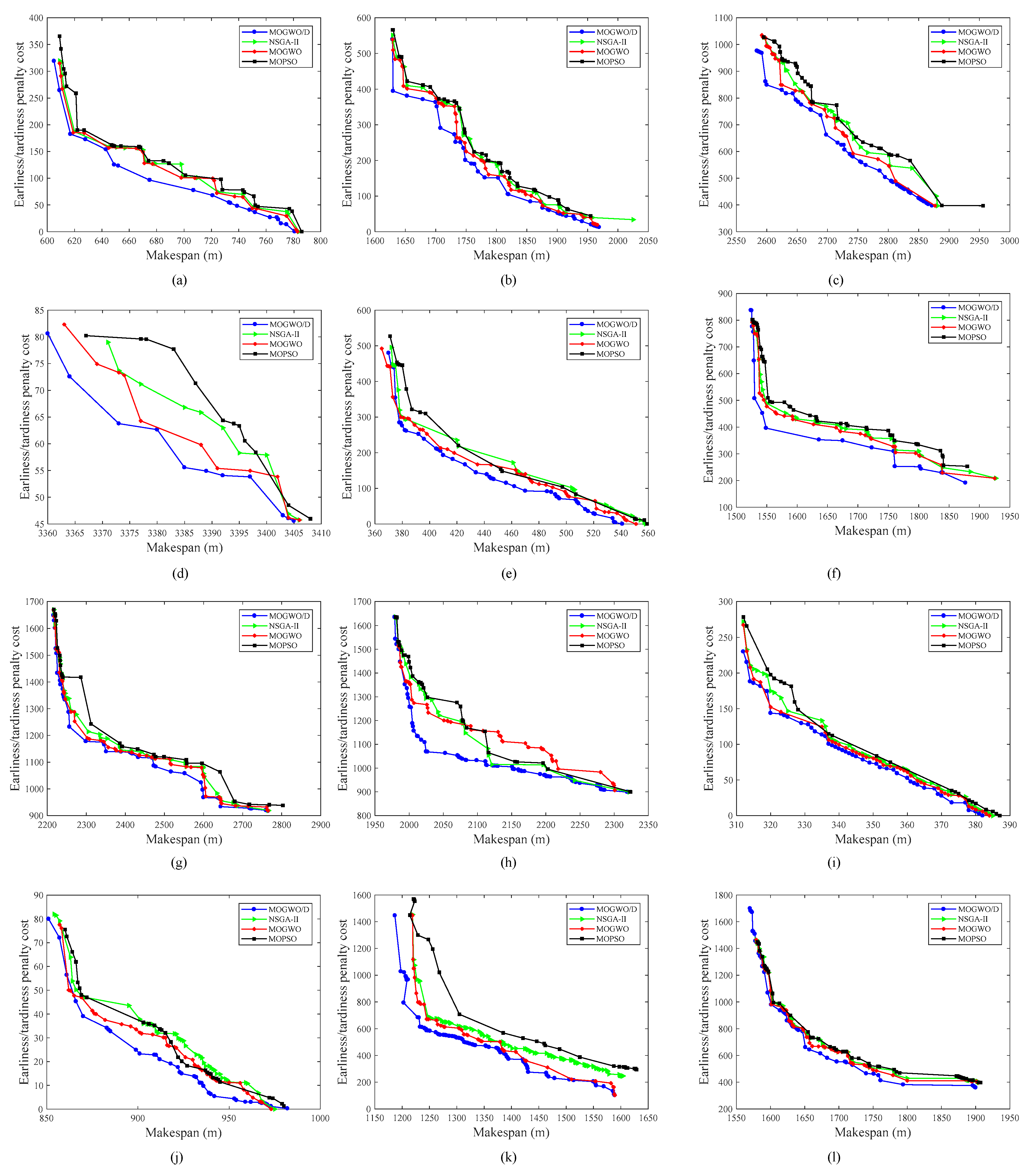
5.4. Experimental Results Analysis

Table 6 presents the means and standard deviations of the three metrics for the MOGWO/D algorithm—NSGA-II, MOGWO, and MOPSO. By comparing the GD, IGD, and Spread values of the four multi-objective algorithms, it can be seen in Table 6 that the proposed MOGWO/D algorithm has better results in the vast majority of instances. Specifically, with regard to the convergence metric GD, the MOGWO/D algorithm achieves the best results for 33 instances; it is inferior to MOGWO on the “2_8_10” and “2_8_20” instances and inferior to MOPSO on “3_4_30”, but the differences are very small. For the spread metric, MOGWO/D algorithm achieves the optimal scheme in 34 instances; it is only inferior to MOGWO on “2_8_10” and inferior to NSGA-II on “3_4_30”, but still better than MOPSO. Regarding the comprehensive metric IGD, 34 instances obtained the best metrics values with the MOGWO/D algorithm, only instance “2_ 8_10” was slightly better when using MOGWO, and NSGA-II is superior to MOGWO/D algorithm on “3_4_30”. Furthermore, the standard deviations achieved for the three metrics for these instances by the MOGWO/D algorithm were better than those of the other three comparison algorithms in the vast majority of instances.
It is clear that the MOGWO/D algorithm has a better optimization performance for solving NPPLS-JP problems, and meets the needs to solve such problems. This may be because of the better balance of the MOGWO/D algorithm between exploitation and exploration, as well as the strategy in which the three best solutions x α , x β , and x δ can be obtained from different levels of the grey wolves’ social hierarchy. The experimental results show that the proposed algorithm is superior to other multi-objective optimization algorithms in solving the NPPLS-JP problem.
To observe the experimental results more intuitively, Figure 5a–j gives the convergence curve of each instance in the instance set, for which the order capacity is 20, and each curve is the best running result according to the comprehensive performance metric IGD over 30 independent runs for the proposed MOGWO/D algorithm and the three other comparison algorithms. It can be seen clearly that the convergence curves of the proposed algorithm are better than those of the comparison algorithms through these curve graphs. Among them, only on instances “3_2_20” and “3_8_20” is the proposed algorithm similar to the comparison algorithms, and the other instances all yield much better convergence curves than those of the comparison algorithms, which proves the effectiveness of the proposed MOGWO/D algorithm in solving the NPPLS-JP problem.
The NPPLS-JP problem proposed in this paper comes from the actual demand of an axle housing machining workshop. This scheduling demand exists widely in a multivariety mixed production environment, so the proposed model and method are of great significance for production practice. This research has a substantive impact on improving the production efficiency of the workshop, and can significantly enhance the production management level of enterprises, so as to increase the market competitiveness.

6. Conclusions

In this paper, a multi-objective NPPLS-JP derived from the real-life axle housing machining workshop of an axle manufacturer is studied. In the established NPPLS-JP model, the structures of all parallel lines are symmetrical. However, because of the demands of multivariety mixed production, the process capabilities and production capacities of these parallel production lines are asymmetric, and some types of job operations must be processed on the specific lines. This situation greatly affects the production efficiency of the production system and increases the difficulty of scheduling. To make multivariety mixed production more efficient and to maximize the utilization of the production capacity, a jumping process operation is introduced into the proposed model, which is the largest difference relative to the other general parallel production line scheduling problems. In the NPPLS-JP model, the multiline scheduling, multivariety mixed production, machine eligibility constraints, and MOPs are involved, so it is an NP-hard scheduling problem. In view of this model, we propose a hybrid multi-objective optimization algorithm that incorporates the single-objective GWO into the MOEA/D. The basic idea is to compensate for the shortcomings of the original algorithms by the reasonable mixing of several algorithms to balance their exploration and exploitation of abilities. To verify the effectiveness of the proposed algorithm, a set of instances is designed, and comparative experiments are conducted using the MOGWO/D algorithm as well as three other famous multi-objective optimization algorithms. The experimental results demonstrate that the proposed algorithm is superior to the compared algorithms for solving the NPPLS-JP problem. Furthermore, the experiment also proves that algorithm mixing can improve the performance and expand the application field of the constitutive algorithms.
In future research, we could solve the NPPLS-JP problem under the condition of considering the sequence-dependent setup times, or we could design new metaheuristics to solve the NPPLS-JP problem. Another interesting research direction is to explore new problem-specific rules to improve the performance of the MOGWO/D algorithm in terms of solving the NPPLS-JP. We can also focus on utilizing the MOGWO/D algorithm to solve other workshop scheduling problems, such as job shop scheduling problems and regular flow shop scheduling problems.

Author Contributions

Conceptualization, L.Y.; Formal analysis, G.X. and J.M.; Investigation, G.X. and J.L.; Methodology, G.X., L.Y. and J.M.; Project administration, Z.G.; Resources, L.Y.; Software, G.X. and J.L.; Writing—original draft, G.X. and L.Y.; Writing—review & editing, L.Y. and J.M.; funding acquisition, L.Y. All authors have read and agreed to the published version of the manuscript.

Funding

This research was funded by the Youth Program of National Natural Science Foundation of China (Grant No. 51905196) and the National Key R&D Program of China (Grant No. 2018YFB1702700).

Institutional Review Board Statement

Not applicable.

Informed Consent Statement

Not applicable.

Data Availability Statement

Not applicable.

Conflicts of Interest

The authors declare that they have no competing interest.

Abbreviations

The mathematical modeling notations are listed as follows.
o the index of orders, o = ( 1 , 2 , , O )
O the number of orders
N o the number of jobs in order o
N J the total number of jobs, N = o = 1 o n o
J a set of jobs, J = { 1 , 2 , , N J }
i , i the index of jobs, i , i J
N L the total number of production lines
L a set of production lines, L = { 1 , 2 , , N L }
l , l the index of production lines, l , l L
N S the number of operations, which is equals to the number of stages
S a set of operations, S = { 1 , 2 , , N S }
s the index of operations, which is also the index of stages, s S
s l the jumping process point of production line l , s l = ( 1 , 2 , , S 1 )
t the index of job types
N t the number of job types
k the index of machines
M l , s the number of machines at stage s of production line l
p t k , t , s the processing time of operation s for a job of type t on machine k
α o the earliness penalty cost coefficient of order o
β o the tardiness penalty cost coefficient of order o
M a sufficiently large positive number
x t , s , l takes a value of 1 if stage s of type t can be processed on production line l and 0 otherwise
x i , o takes a value of 1 if job i is included in order o and 0 otherwise
x o , t takes a value of 1 if the type of jobs in order o is t and 0 otherwise
( d o 1 , d o 2 , d o 3 , d o 4 ) the trapezoidal fuzzy number for trapezoidal fuzzy due date of order o , where d o 1 d o 2 d o 3 d o 4
Decision variables
X i , s , l binary variable, taking a value of 1 if operation s of job i is processed on production line l and 0 otherwise
X k , s , i , l binary variable, taking a value of 1 if operation s and s of job i are both processed on production line l and 0 otherwise
Y i , s , s binary variable, taking a value of 1 if operation s of job i is processed before job i on machine k of production line l and 0 otherwise
Z k , i , i , s , l binary variable, taking a value of 1 if operation s of job i is processed before job i on machine k of production line l and 0 otherwise
C k , s , i , l the completion time of operation s of job i on machine k of production line l
C o   the completion time for order o
P o the fuzzy due date earliness/tardiness penalty cost of order o

References

  1. Mohammadi, M.; Ghomi, S.; Jafari, N. A genetic algorithm for simultaneous lotsizing and sequencing of the permutation flow shops with sequence-dependent setups. Int. J. Comput. Integr. Manuf. 2011, 24, 87–93. [Google Scholar] [CrossRef]
  2. Varmazyar, M.; Salmasi, N. Sequence-dependent flow shop scheduling problem minimising the number of tardy jobs. Int. J. Prod. Res. 2012, 50, 5843–5858. [Google Scholar] [CrossRef]
  3. Yue, L.; Guan, Z.; Zhang, L.; Ullah, S.; Cui, Y. Multi objective lotsizing and scheduling with material constraints in flexible parallel lines using a Pareto based guided artificial bee colony algorithm. Comput. Ind. Eng. 2019, 128, 659–680. [Google Scholar] [CrossRef]
  4. Jungwattanakit, J.; Reo De Cha, M.; Chaovalitwongse, P.; Werner, F. A comparison of scheduling algorithms for flexible flow shop problems with unrelated parallel machines, setup times, and dual criteria. Comput. Oper. Res. 2009, 36, 358–378. [Google Scholar] [CrossRef]
  5. Low, C. Simulated annealing heuristic for flow shop scheduling problems with unrelated parallel machines. Comput. Oper. Res. 2005, 32, 2013–2025. [Google Scholar] [CrossRef]
  6. Soltani, S.A.; Karimi, B. Cyclic hybrid flow shop scheduling problem with limited buffers and machine eligibility constraints. Int. J. Adv. Manuf. Technol. 2014, 76, 1739–1755. [Google Scholar] [CrossRef]
  7. Tadayon, B.; Salmasi, N. A two-criteria objective function flexible flowshop scheduling problem with machine eligibility constraint. Int. J. Adv. Manuf. Technol. 2013, 64, 1001–1015. [Google Scholar] [CrossRef]
  8. Ruiz, R.; Maroto, C. A genetic algorithm for hybrid flowshops with sequence dependent setup times and machine eligibility. Eur. J. Oper. Res. 2007, 169, 781–800. [Google Scholar] [CrossRef]
  9. Zhang, X.Y.; Chen, L. A re-entrant hybrid flow shop scheduling problem with machine eligibility constraints. Int. J. Prod. Res. 2018, 56, 5293–5305. [Google Scholar] [CrossRef]
  10. Oddi, A.; Rasconi, R.; Cortellessa, G.; Magazzeni, D.; Maratea, M.; Serina, I. Leveraging constraint-based approaches formulti-objective flexible flow-shop scheduling with energy costs. Intell. Artif. 2016, 10, 147–160. [Google Scholar]
  11. Méndez, C.A.; Henning, G.P.; Cerdá, J. An MILP continuous-time approach to short-term scheduling of resource-constrained multistage flowshop batch facilities. Comput. Chem. Eng. 2001, 25, 701–711. [Google Scholar] [CrossRef]
  12. Malik, A.I.; Kim, B.S. A multi-constrained supply chain model with optimal production rate in relation to quality of products under stochastic fuzzy demand. Comput. Ind. Eng. 2020, 149, 106814. [Google Scholar] [CrossRef]
  13. Malik, A.I.; Sarkar, B. Coordinating supply-chain management under stochastic fuzzy environment and lead-time reduction. Mathematics 2019, 7, 480. [Google Scholar] [CrossRef] [Green Version]
  14. Wu, H.C. Solving the fuzzy earliness and tardiness in scheduling problems by using genetic algorithms. Expert Syst. Appl. 2010, 37, 4860–4866. [Google Scholar] [CrossRef]
  15. Bukchin, J.; Dar-El, E.M.; Rubinovitz, J. Mixed model assembly line design in a make-to-order environment. Comput. Ind. Eng. 2002, 41, 405–421. [Google Scholar] [CrossRef]
  16. Caridi, M.; Sianesi, A. Multi-Agent Systems in production planning and control: An application to the scheduling of mixed-model assembly lines. Int. J. Prod. Econ. 2000, 68, 29–42. [Google Scholar] [CrossRef]
  17. Askin, R.G.; Zhou, M. A parallel station heuristic for the mixed-model production line balancing problem. Int. J. Prod. Res. 1997, 35, 3095–3106. [Google Scholar] [CrossRef]
  18. Emde, S.; Boysen, N. Optimally locating in-house logistics areas to facilitate JIT-supply of mixed-model assembly lines. Int. J. Prod. Econ. 2010, 135, 393–402. [Google Scholar] [CrossRef]
  19. Lopes, T.C.; Michels, A.S.; Sikora, C.; Magatão, L. Balancing and cyclical scheduling of asynchronous mixed-model assembly lines with parallel stations. J. Manuf. Syst. 2019, 50, 193–200. [Google Scholar] [CrossRef]
  20. Zhao, X.; Liu, J.; Ohno, K.; Kotani, S. Modeling and analysis of a mixed-model assembly line with stochastic operation times. Nav. Res. Logist. 2010, 54, 681–691. [Google Scholar] [CrossRef]
  21. Khalid, Q.S.; Arshad, M.; Maqsood, S.; Kim, S. Hybrid particle swarm algorithm for products’ scheduling problem in cellular manufacturing system. Symmetry 2019, 11, 729. [Google Scholar] [CrossRef] [Green Version]
  22. Mcmullen, P.R.; Tarasewich, P. A beam search heuristic method for mixed-model scheduling with setups. Int. J. Prod. Econ. 2005, 96, 273–283. [Google Scholar] [CrossRef]
  23. Leu, S.S.; Hwang, S.T. GA-based resource-constrained flow-shop scheduling model for mixed precast production. Autom. Constr. 2002, 11, 439–452. [Google Scholar] [CrossRef]
  24. Wang, B.; Guan, Z.; Ullah, S.; Xu, X.; He, Z. Simultaneous order scheduling and mixed-model sequencing in assemble-to-order production environment: A multi-objective hybrid artificial bee colony algorithm. J. Intell. Manuf. 2017, 28, 419–436. [Google Scholar] [CrossRef]
  25. Bahman, N.; Ahmed, A.; Katayoun, B. A realistic multi-manned five-sided mixed-model assembly line balancing and scheduling problem with moving workers and limited workspace. Int. J. Prod. Res. 2019, 57, 643–661. [Google Scholar]
  26. Alghazi, A.; Kurz, M.E. Mixed model line balancing with parallel stations, zoning constraints, and ergonomics. Constraints 2018, 23, 123–153. [Google Scholar] [CrossRef]
  27. Rajeswari, N.; Shahabudeen, P. Bicriteria parallel flow line scheduling using hybrid population-based heuristics. Int. J. Adv. Manuf. Technol. 2009, 43, 799–804. [Google Scholar] [CrossRef]
  28. Haq, A.N.; Balasubramanian, K.; Sashidharan, B.; Karthick, R.B. Parallel line job shop scheduling using genetic algorithm. Int. J. Adv. Manuf. Technol. 2008, 35, 1047–1052. [Google Scholar]
  29. Meyr, H.; Mann, M. A decomposition approach for the general lotsizing and scheduling problem for parallel production lines. Eur. J. Oper. Res. 2013, 229, 718–731. [Google Scholar] [CrossRef]
  30. Mumtaz, J.; Guan, Z.; Yue, L.; Zhang, L.; He, C. Hybrid spider monkey optimisation algorithm for multi-level planning and scheduling problems of assembly lines. Int. J. Prod. Res. 2020, 58, 6252–6267. [Google Scholar] [CrossRef]
  31. Ebrahimipour, V.; Najjarbashi, A.; Sheikhalishahi, M. Multi-objective modeling for preventive maintenance scheduling in a multiple production line. J. Intell. Manuf. 2013, 26, 1–12. [Google Scholar] [CrossRef]
  32. Mumtaz, J.; Guan, Z.; Yue, L.; Wang, Z.; Rauf, M. Multi-level planning and scheduling for parallel pcb assembly lines using hybrid spider monkey optimization approach. IEEE Access 2019, 7, 2169–3536. [Google Scholar] [CrossRef]
  33. Liu, Z.Z.; Wang, Y.; Huang, P.Q. A many-objective evolutionary algorithm with angle-based selection and shift-based density estimation. Inf. Sci. 2017, 509, 400–419. [Google Scholar] [CrossRef] [Green Version]
  34. Goldberg, D.E.; Korb, B.; Deb, K. Messy genetic algorithms: Motivation, analysis, and first results. Complex Syst. 1989, 3, 493–530. [Google Scholar]
  35. Zitzler, E.; Thiele, L. Multiobjective evolutionary algorithms: A comparative case study and the strength Pareto approach. IEEE Trans. Evol. Comput. 1999, 3, 257–271. [Google Scholar] [CrossRef] [Green Version]
  36. Zitzler, E.; Laumanns, M.; Thiele, L. SPEA2: Improving the Performance of the Strength Areto Evolutionary Algorithm; Evolutionary Methods for Design, Optimization and Control with Applications to Industrial Problems (EUROGEN 2001), Athens, Greece, September; Giannakoglou, K.C., Tsahalis, D.T., Périaux, J., Papailiou, K.D., Fogarty, T., Eds.; International Center for Numerical Methods in Engineering (CIMNE): Barcelona, Spain, 2002; pp. 95–100. [Google Scholar]
  37. Deb, K.; Pratap, A.; Agarwal, S.; Meyarivan, T. A fast and elitist multiobjective genetic algorithm: NSGA-II. IEEE Trans. Evol. Comput. 2002, 6, 182–197. [Google Scholar] [CrossRef] [Green Version]
  38. Beume, N.; Naujoks, B.; Emmerich, M. Sms-emoa: Multiobjective selection based on dominated hypervolume. Eur. J. Oper. Res. 2007, 181, 1653–1669. [Google Scholar] [CrossRef]
  39. Bader, J.; Zitzler, E. Hype: An algorithm for fast hypervolume-based many-objective optimization. Evol. Comput. 2011, 19, 45–76. [Google Scholar] [CrossRef] [PubMed]
  40. Zhang, Q.; Hui, L. MOEA/D: A multiobjective evolutionary algorithm based on decomposition. IEEE Trans. Evol. Comput. 2007, 11, 712–731. [Google Scholar] [CrossRef]
  41. Li, H.; Landa-Silva, D. An adaptive evolutionary multi-objective approach based on simulated annealing. Evol. Comput. 2014, 19, 561–595. [Google Scholar] [CrossRef] [PubMed] [Green Version]
  42. Tan, Y.Y.; Jiao, Y.C.; Hong, L.; Wang, X.K. MOEA/D-SQA: A multi-objective memetic algorithm based on decomposition. Eng. Optim. 2012, 44, 1–21. [Google Scholar] [CrossRef]
  43. Cai, D.; Yuping, W.; Miao, Y. A new multi-objective particle swarm optimization algorithm based on decomposition. Inf. Sci. 2015, 325, 541–557. [Google Scholar]
  44. Ke, L.; Zhang, Q.; Battiti, R. MOEA/D-ACO: A Multiobjective Evolutionary Algorithm Using Decomposition and Antcolony. IEEE Trans. Cybern. 2013, 43, 1845–1859. [Google Scholar] [CrossRef] [PubMed]
  45. Alhindi, A.; Alhindi, A.; Alhejali, A.; Alsheddy, A.; Tairan, N.; Alhakami, H. MOEA/D-GLS: A multiobjective memetic algorithm using decomposition and guided local search. Soft Comput. 2019, 23, 9605–9615. [Google Scholar] [CrossRef]
  46. Zhang, Q.; Liu, W.; Tsang, E.; Virginas, B. Expensive multiobjective optimization by MOEA/D with gaussian process model. IEEE Trans. Evol. Comput. 2010, 14, 456–474. [Google Scholar] [CrossRef]
  47. Wang, Z.; Zhang, Q.; Zhou, A.; Gong, M.; Jiao, L. Adaptive replacement strategies for MOEA/D. IEEE Trans. Cybern. 2017, 46, 474–486. [Google Scholar] [CrossRef]
  48. Ho, Y.C.; Pepyne, D.L. Simple explanation of the no-free-lunch theorem and its implications. J. Optim. Theory Appl. 2002, 115, 549–570. [Google Scholar] [CrossRef]
  49. Murata, T.; Gen, M.; Ishibuchi, H. Multi-objective scheduling with fuzzy due-date. Comput. Ind. Eng. 1998, 35, 439–442. [Google Scholar] [CrossRef]
  50. Vela, C.R.; Afsar, S.; Palacios, J.J.; González-Rodríguez, I.; Puente, J. Evolutionary tabu search for flexible due-date satisfaction in fuzzy job shop scheduling. Comput. Oper. Res. 2020, 119, 104931. [Google Scholar] [CrossRef]
  51. Wen, X.; Li, X.; Gao, L.; Wang, K.; Li, H. Modified honey bees mating optimization algorithm for multi-objective uncertain integrated process planning and scheduling problem. Int. J. Adv. Robot. Syst. 2020, 17, 172988142092523. [Google Scholar] [CrossRef]
  52. Mirjalili, S.; Mirjalili, S.M.; Lewis, A. Grey Wolf Optimizer. Adv. Eng. Softw. 2014, 69, 46–61. [Google Scholar] [CrossRef] [Green Version]
  53. Scheffé, H. Experiments with Mixtures. J. Roy. Statist. Soc. 1958, 20, 344–360. [Google Scholar] [CrossRef]
  54. Li, B.B.; Wang, L.; Liu, B. An effective PSO-based hybrid algorithm for multiobjective permutation flow shop scheduling. IEEE Trans. Syst. Man Cybern. Paart A Syst. Hum. 2008, 38, 818–831. [Google Scholar] [CrossRef]
  55. Mirjalili, S.; Saremi, S.; Mirjalili, S.M.; Coelho, L. Multi-objective grey wolf optimizer: A novel algorithm for multi-criterion optimization. Expert Syst. Appl. 2015, 47, 106–119. [Google Scholar] [CrossRef]
  56. Coello, C.A.C.; Pulido, G.T.; Lechuga, M.S. Handling multiple objectives with particle swarm optimization. IEEE Trans. Evol. Comput. 2004, 8, 256–279. [Google Scholar] [CrossRef]
  57. Zitzler, E.; Thiele, L.; Laumanns, M.; Fonseca, C.M.; Fonseca, V. Performance assessment of multiobjective optimizers: An analysis and review. IEEE Trans. Evol. Comput. 2003, 7, 117–132. [Google Scholar] [CrossRef] [Green Version]
  58. Jiang, S.; Ong, Y.; Zhang, J.; Feng, L. Consistencies and contradictions of performance metrics in multiobjective optimization. IEEE Trans. Cybern. 2014, 44, 2391–2404. [Google Scholar] [CrossRef] [PubMed]
  59. Oguz, C.; Ercan, M.F. A genetic algorithm for hybrid flow-shop scheduling with multiprocessor tasks. Complex Syst. 2005, 8, 323–351. [Google Scholar]
Figure 1. The composition of an axle housing machining line.
Symmetry 13 01521 g001
Figure 2. The earliness/tardiness penalty cost and satisfaction model. (a) The earliness/tardiness penalty cost; (b) The satisfaction model.
Symmetry 13 01521 g002
Figure 3. An example of decoding.
Symmetry 13 01521 g003
Figure 4. The three different production scenarios. (a) Scenario 1; (b) Scenario 2; (c) Scenario 3.
Symmetry 13 01521 g004
Figure 5. The convergence curves for the instance set with z = 20. (a) 1_2_20; (b) 1_4_20; (c) 1_6_20; (d) 1_8_20; (e) 2_2_20; (f) 2_4_20; (g) 2_6_20; (h) 2_8_20; (i) 3_2_20; (j) 3_4_20; (k) 3_6_20; (l) 3_8_20.
Symmetry 13 01521 g005
Table 1. The data used in the example.
Order No.Number of JobsJob Type
123
231
312
Table 2. The line selection information of the example.
Job TypesAvailable QuantityOptional Lines
012
1212
23123
33123
Table 3. The optional machines and the processing times for each type of job.
Job
Types
Stage 1Stage 2Stage 3Stage 4Stage 5
M 1 M 2 M 3 M 4 M 5 M 6 M 7 M 8 M 9 M 10 M 11 M 12 M 13 M 14 M 15 M 16 M 17 M 18 M 19 M 20
1414130303939343442423131 262649492323
2404031314242343440403232 232350502323
34040323238383232414132324747262652522424
43939323241413232393929294848262652522424
5424234344040343439393030 242451512424
6404035353939313142423131 232346462222
73939323240403232404033335454242454542424
84343313142423131434334345757262656562626
Table 4. Production line selection information for the experiments.
TypeAvailable QuantityOptional Lines
012
1223-
2223-
33123
43123
5323-
6323-
73123
83123
Table 5. The parameter settings for the four algorithms.
MOGWO/DNSGA-IIMOGWOMOPSO
Population size (N): 60
and iterations: 300
(20 and 40 jobs)
Population size (N): 60
and iterations: 300
(20 and 40 jobs)
Population size ( N ): 60
and iterations: 300
(20 and 40 jobs)
Population size ( N ): 60
and iterations: 300
(20 and 40 jobs)
Population size ( N ): 100
and iterations: 500
(60 and 80 jobs)
Population size (N): 100
and iterations: 500
(60 and 80 jobs)
Population size ( N ): 100
and iterations: 500
(60 and 80 jobs)
Population size ( N ): 100
and iterations: 500
(60 and 80 jobs)
Population size ( N ): 240
and iterations: 800
(120 and 160 jobs)
Population size ( N ): 240
and iterations: 800
(120 and 160 jobs)
Population size ( N ): 240
and iterations: 800
(120 and 160 jobs)
Population size ( N ): 240
and iterations: 800
(120 and 160 jobs)
Population size ( N ): 300
and iterations: 1000
(180 and 240 jobs)
Population size ( N ): 300
and iterations: 1000
(180 and 240 jobs)
Population size( N ): 300
and iterations: 1000
(180 and 240 jobs)
Population size ( N ): 300
and iterations: 1000
(180 and 240 jobs)
The external population size: N Crossover rate: 0.9The external population size: N The external archive size: N
The neighborhood size: 20 (for all instances)Mutation rate: 0.1 The inertia weight wo = 0.4
T = 6 (for all instances) The acceleration coefficients c 1 = c 2 = 2.0
Table 6. Means and deviations of the three metrics obtained by MOGWO/D, NSGA-II, MOGWO, and MOPSO.
ProblemsMOGWO/DNSGA-IIMOGWOMOPSO
GDIGD Δ GDIGD Δ GDIGD Δ GDIGD Δ
1_2_103.11E-23.93E-32.62E-17.52E-21.20E-27.96E-16.52E-21.02E-27.56E-18.50E-21.33E-27.70E-1
6.73E-38.93E-44.68E-28.07E-31.62E-38.51E-27.80E-32.01E-3/6.50E-1.06E-21.67E-37.80E-2
1_4_101.38E-24.36E-33.57E-13.32E-21.47E-28.15E-12.86E-21.18E-28.62E-13.82E-21.69E-27.71E-1
5.11E-31.03E-36.08E-21.05E-23.66E-31.00E-19.12E-33.19E-39.77E-21.32E-23.93E-37.77E-2
1_6_107.45E-32.09E-36.24E-15.82E-28.47E-37.61E-12.96E-24.17E-37.50E-18.15E-21.08E-26.43E-1
9.70E-36.04E-46.19E-26.83E-21.19E-25.64E-13.16E-23.61E-35.55E-11.29E-11.68E-25.35E-1
1_8_101.70E-31.05E-33.90E-18.44E-34.70E-38.74E-14.62E-3 2.88E-38.31E-11.27E-26.14E-36.97E-1
8.40E-44.09E-42.95E-23.99E-33.14E-32.23E-11.72E-31.26E-35.83E-21.06E-25.77E-34.15E-1
1_2_202.36E-21.74E-23.81E-13.46E-24.84E-21.01E + 003.94E-24.60E-21.02E + 002.54E-25.02E-29.70E-1
3.96E-28.09E-31.95E-14.16E-25.90E-37.97E-24.96E-29.25E-31.44E-12.30E-23.68E-34.40E-2
1_4_201.12E-24.20E-33.64E-12.20E-21.02E-27.68E-12.00E-29.37E-37.80E-12.48E-21.11E-27.60E-1
5.60E-32.48E-34.85E-28.89E-34.67E-34.50E-28.78E-34.78E-35.88E-21.04E-24.81E-38.10E-2
1_6_203.49E-21.94E-24.68E-13.59E + 014.37E-29.65E-13.83E + 014.08E-29.36E-13.74E + 014.69E-29.96E-1
1.56E-24.78E-37.30E-21.32E + 021.05E-21.97E-11.43E + 021.04E-22.23E-11.27E + 021.32E-22.16E-1
1_8_203.02E + 013.22E-35.40E-18.49E + 017.62E-38.48E-17.42E + 017.19E-39.86E-19.41E + 019.05E-37.21E-1
6.97E + 012.23E-39.90E-21.69E + 026.33E-35.76E-11.67E + 025.32E-34.56E-11.69E + 027.71E-36.13E-1
1_2_304.34E-25.87E-31.93E-11.51E-11.69E-27.50E-11.16E-11.45E-27.12E-11.77E-11.89E-27.55E-1
2.94E-21.03E-37.06E-23.79E-23.32E-31.02E-13.69E-22.81E-39.66E-23.80E-23.85E-31.00E-1
1_4_303.26E-21.08E-23.92E-15.55E-22.68E-28.50E-15.43E-22.41E-28.14E-15.57E-22.82E-28.27E-1
1.98E-27.54E-35.74E-22.93E-21.55E-26.21E-23.06E-21.54E-27.18E-22.82E-21.54E-26.66E-2
1_6_304.64E + 011.60E-14.35E-16.90E + 013.61E-1 8.93E-15.37E + 013.44E-18.81E-11.23E + 023.75E-1 9.42E-1
2.02E + 029.72E-26.76E-23.00E + 022.10E-11.23E-12.33E + 022.10E-11.44E-14.29E + 022.12E-11.51E-1
1_8_301.76E + 023.22E + 006.02E-13.62E + 021.07E + 011.28E + 002.77E + 028.59E + 001.29E + 003.94E + 021.50E + 011.27E + 00
1.35E + 024.78E + 007.64E-21.71E + 021.10E + 016.85E-21.74E + 021.05E + 011.12E-11.84E + 021.06E + 015.52E-2
2_2_101.69E-31.05E-33.76E-16.66E-35.14E-31.02E + 004.83E-33.34E-38.82E-19.05E-37.88E-31.14E + 00
3.88E-41.91E-43.07E-29.63E-48.87E-48.09E-28.66E-44.83E-47.77E-21.57E-32.14E-36.75E-2
2_4_107.71E-39.17E-44.50E-13.38E-25.39E-38.93E-12.75E-23.31E-39.12E-14.15E-27.50E-39.21E-1
5.79E-34.21E-45.34E-22.28E-22.90E-39.24E-21.53E-26.50E-49.76E-23.02E-25.06E-38.74E-2
2_6_101.60E-13.14E-25.50E-12.21E-16.49E-28.99E-12.05E-15.64E-28.87E-12.37E-17.13E-29.23E-1
1.30E-15.50E-31.04E-11.05E-19.55E-31.09E-11.18E-18.56E-39.91E-21.04E-19.18E-31.13E-1
2_8_101.04E-33.60E-36.16E-11.03E-31.04E-35.81E-21.37E-43.20E-45.46E-27.52E-42.21E-34.89E-2
2.20E-41.69E-35.64E-24.49E-34.53E-32.53E-15.96E-41.40E-32.38E-13.28E-39.64E-32.13E-1
2_2_201.26E-37.85E-43.51E-12.74E-21.50E-21.11E + 009.37E-33.80E-39.47E-13.72E-22.48E-21.28E + 00
4.72E-41.52E-42.68E-22.04E-27.67E-31.18E-14.89E-35.08E-49.58E-22.59E-28.00E-32.26E-1
2_4_206.34E-32.90E-34.98E-12.15E-29.74E-31.05E + 001.55E-26.88E-31.03E + 002.68E-29.90E-39.77E-1
4.19E-31.71E-35.70E-21.48E-26.84E-31.52E-17.67E-32.89E-31.40E-11.37E-26.18E-32.52E-1
2_6_201.67E-28.88E-35.86E-12.19E-21.60E-29.59E-11.86E-21.45E-29.07E-12.81E-21.85E-29.74E-1
6.75E-33.72E-34.58E-27.23E-35.75E-35.46E-25.82E-35.77E-36.54E-29.63E-36.00E-37.60E-2
2_8_201.89E-21.88E-26.05E-12.26E-23.12E-29.34E-12.16E-22.95E-29.08E-12.56E-23.28E-29.84E-1
9.36E-39.15E-36.20E-29.38E-31.41E-28.92E-28.77E-31.38E-29.37E-21.17E-21.43E-21.13E-1
2_2_301.07E-39.50E-44.10E-18.16E-39.67E-31.12E + 005.01E-35.72E-39.80E-11.22E-21.46E-21.24E + 00
5.40E-44.77E-44.66E-24.11E-38.56E-32.01E-13.22E-35.86E-31.80E-14.87E-38.92E-31.63E-1
2_4_301.75E-21.65E-24.80E-12.22E-22.91E-28.30E-12.08E-22.78E-28.44E-12.35E-23.04E-28.43E-1
1.63E-29.82E-36.57E-21.55E-22.00E-22.98E-11.47E-21.97E-23.17E-11.63E-22.03E-23.02E-1
2_6_309.06E-35.89E-36.22E-11.24E-29.63E-39.98E-11.10E-29.27E-39.70E-11.39E-29.81E-31.01E + 00
6.63E-33.02E-37.22E-27.18E-34.56E-38.25E-27.36E-34.69E-38.23E-27.24E-34.29E-38.61E-2
2_8_301.40E-22.55E-26.39E-11.54E-24.10E-21.00E + 001.55E-24.00E-21.03E + 001.62E-24.18E-21.02E + 00
5.97E-39.17E-34.74E-25.50E-31.45E-27.58E-25.57E-31.45E-27.57E-25.85E-31.47E-26.46E-2
3_2_103.81E-32.44E-32.93E-17.36E-37.38E-36.54E-16.53E-36.16E-36.26E-18.96E-38.81E-36.70E-1
5.73E-41.96E-43.01E-26.19E-47.85E-46.62E-26.45E-44.02E-44.89E-29.92E-41.10E-34.24E-2
3_4_101.75E-34.21E-36.30E-11.80E-23.63E-21.03E + 001.48E-22.00E-21.13E + 001.68E-24.94E-21.01E + 00
1.65E-39.72E-45.37E-21.96E-21.55E-21.44E-11.58E-21.23E-21.05E-11.66E-24.51E-36.04E-2
3_6_103.05E-32.02E-35.03E-13.45E-21.69E-29.37E-11.35E-28.79E-31.01E + 004.13E-21.33E-26.96E-1
2.82E-31.20E-37.36E-22.52E-21.63E-23.19E-18.74E-35.07E-32.55E-14.68E-21.35E-24.67E-1
3_8_108.48E-48.06E-44.09E-12.30E-21.55E-21.09E + 004.49E-33.82E-31.01E + 003.23E-21.80E-28.86E-1
4.96E-44.08E-43.25E-21.70E-21.20E-22.93E-12.69E-32.88E-31.40E-13.31E-21.52E-25.31E-1
3_2_203.22E-39.19E-43.59E-12.72E-21.32E-21.14E + 001.40E-24.41E-39.26E-13.86E-22.67E-21.29E + 00
1.27E-31.41E-43.27E-28.04E-34.61E-39.75E-24.02E-31.22E-39.68E-21.02E-24.68E-31.31E-1
3_4_204.37E-39.39E-43.66E-11.32E-23.46E-38.24E-19.38E-32.58E-38.42E-11.89E-24.74E-38.89E-1
2.73E-31.84E-47.22E-26.55E-36.67E-41.14E-15.05E-34.39E-41.11E-19.37E-38.16E-41.16E-1
3_6_206.68E-33.27E-35.18E-11.88E-29.60E-31.07E + 001.47E-28.03E-31.05E + 002.63E-21.29E-21.08E + 00
4.66E-31.89E-34.42E-29.13E-34.32E-31.18E-17.62E-33.77E-37.74E-21.91E-25.64E-31.27E-1
3_8_202.79E-31.74E-34.18E-19.66E-36.78E-39.36E-18.24E-35.52E-39.39E-11.63E-21.28E-21.01E + 00
2.21E-31.28E-34.86E-24.76E-34.90E-32.91E-15.74E-36.58E-31.19E-11.59E-21.33E-22.97E-1
3_2_303.92E-33.23E-32.34E-11.19E-21.08E-25.27E-11.00E-28.67E-35.25E-11.39E-21.34E-25.42E-1
1.48E-33.54E-44.10E-25.13E-37.11E-41.04E-16.26E-36.82E-41.67E-13.99E-38.41E-41.09E-1
3_4_303.24E-21.14E-21.30E-13.05E-32.14E-31.31E-14.24E-34.28E-31.79E-12.39E-33.05E-31.49E-1
8.88E-32.88E-36.68E-29.15E-36.46E-33.94E-19.13E-39.65E-34.35E-19.50E-39.34E-34.47E-1
3_6_308.38E-31.36E-25.02E-11.76E-21.76E-24.33E-13.87E-23.30E-27.28E-12.12E-22.43E-24.22E-1
3.06E-35.69E-35.45E-23.95E-23.05E-25.44E-16.29E-23.14E-24.95E-14.61E-23.89E-25.25E-1
3_8_301.76E-21.20E-24.68E-13.21E-22.64E-21.02E + 002.79E-22.50E-21.04E + 004.39E-22.84E-21.02E + 00
9.12E-34.95E-35.92E-21.45E-21.03E-21.18E-11.23E-29.90E-31.10E-13.48E-21.08E-21.38E-1
Statistics33/3034/3435/330/11/00/12/31/11/01/20/10/2
Publisher’s Note: MDPI stays neutral with regard to jurisdictional claims in published maps and institutional affiliations.

