On Normalized Laplacians, Degree-Kirchhoff Index and Spanning Tree of Generalized Phenylene

Abstract

The normalized Laplacian is extremely important for analyzing the structural properties of non-regular graphs. The molecular graph of generalized phenylene consists of n hexagons and $2n$ squares, denoted by $L_n^{6,4,4}$. In this paper, by using the normalized Laplacian polynomial decomposition theorem, we have investigated the normalized Laplacian spectrum of $L_n^{6,4,4}$ consisting of the eigenvalues of symmetric tri-diagonal matrices ${\mathcal{L}}_A$ and ${\mathcal{L}}_S$ of order $4n+1$. As an application, the significant formula is obtained to calculate the multiplicative degree-Kirchhoff index and the number of spanning trees of generalized phenylene network based on the relationships between the coefficients and roots.

1. Introduction and Preliminaries

In this paper, only simple, undirected, and finite graphs are considered. Assume that $G=(V_G,E_G)$ is a graph with vertex set $V_G$ and edge set $E_G$. The order of G is denoted by $n=|V_G|$ and the size of G is denoted by $m=|E_G|$. The fundamental expressions and methodologies of graph theory have been used (see [1]). Assume that G is a graph of n vertices, adjacency matrix$A_G={\left[a_{ij}\right]}_{n\times n}$ is a matrix, such that $a_{ij}$ equals 1 if vertices $v_i$ and $v_j$ are adjacent and zero for otherwise. Assume that $D_G=diag(d_{v_1},\dots ,d_{v_n})$ is the vertex degree diagonal matrix of order $n,$ where $d_{v_i}$ is the degree of $v_i,$$1\le i\le n.$ Then $L_G=D_G-A_G$ is called the (combinational) Laplacian matrix of G.

The traditional concept of distance between vertices $v_i$ and $v_j$, is the length of the shortest path obtained by joining these vertices of graph G and that is denoted by $d_{ij}=d_G(v_i,v_j)$. In graph theory, distance is also an essential invariant from which distance based parameters are obtained. In [2], a well-known distance based parameter named as Wiener index and denoted by $W_G$ is introduced for the first time. This parameter is obtained by adding the distances between every pair of vertices in G, that is, $W_G={\sum }_{\{v_i,v_j\}\subseteq V_G}{d}_{ij}$. Eventually, Gutman [3] also developed the Gutman index, which is a weighted variant of the Wiener index and defined as $Gut\left(G\right)={\sum }_{\{v_i,v_j\}\subseteq V_G}{d}_i{d}_j{d}_{ij}$.

In [4], Klein and Randić suggested a novel distance function $r_{ij}$ for a graph depending upon the electrical network theory, which is called the resistance distance. The Kirchhoff index was generated by Klein and Ivanciuc [5] and Klein and Randi [4] based on the resistance distance parameter and is denoted by $Kf\left(G\right)={\sum }_{\{v_i,v_j\}\subseteq V_G}{r}_{ij}$.

Gutman and Mohar [6] established a result separately for the Kirchhoff index that is represented as,

$$Kf\left(G\right)=\sum _{i<j}{r}_{ij}=n{\displaystyle \sum _{i=2}^n}{\frac{1}{\mu }}_i$$

(1)

where ${\mu }_1<{\mu }_2\le \cdots \le {\mu }_n$ with ${\mu }_1=0$ and $n\ge 2$ are the eigenvalues of $L_G$.

In [7], Chung proposed the normalized Laplacian, denoted by ${\mathcal{L}}_G$, that is, ${\mathcal{L}}_G=I-D_G^{\frac{1}{2}}\left(D_G^{-1}A\right)D_G^{-\frac{1}{2}}=D_G^{-\frac{1}{2}}{L}_G{D}_G^{-\frac{1}{2}}$ As a result, it is easy to understand that

$${\left({\mathcal{L}}_G\right)}_{ij}=\left\{\begin{array}{cc}1,\hfill & \mathrm{if}i=j;\hfill \\ -\frac{1}{\sqrt{d_i{d}_j}},\hfill & \mathrm{if}i\ne j,v_i\sim v_j;\hfill \\ 0,\hfill & otherwise,\hfill \end{array}\right.$$

(2)

where $d_i$ ($d_j$) be the degree of the vertex $v_i$ ($v_j$) and ${\left({\mathcal{L}}_G\right)}_{ij}$ show the $(i,j)$-th values of ${\mathcal{L}}_G$. In $2007,$ Chen and Zhang [8] presented a new index based on normalized Laplacian, which is called the multiplicative degree-Kirchhoff index and defined it as, $K{f}^{*}\left(G\right)=2\left|E_G\right|{\sum }_{i=2}^n\frac{1}{{\lambda }_i}$. Moreover, the Kirchhoff index has gained much attention due to its widespread use in chemistry, physics, mathematics, and theoretical computer science. Many scientists have previously proposed new closed formulae of Kirchhoff and multiplicative degree-Kirchhoff indies, along with linear polyomino chains [9], circulant graphs [10], quadrilateral graphs [11], cycles [12], composite graphs [13], and so on. There are several results on the degree-Kirchhoff index and normalized Laplacian (see [14,15,16,17,18,19,20,21,22,23,24,25]).

Due to the widely applications, the molecular graphs phenylenes, pentagonal, hexagonal, and octagonal networks have attracted strong interests of chemists, mathematicians, and engineering. Phenylenes are two connected graphs with structure-property that each of their cells (or interior faces) has become a hexagon or square with the same edge length. Phenylene systems are essential in theoretical chemistry because they can reflect a hydrocarbon in nature. In [26,27], Gutman et al. addressed the phenylene enumeration problem using the Kekulé structure. Later, Pavlović and Gutman [28] have solved the problem of evaluating the Wiener index of phenylenes. Chen and Zhang [29] calculated the expected value of Wiener index (or the number of perfect matches) of the unique phenylene chain using a specific analytical expression. Recently, Geng and Lei [30] explicitly calculated the Kirchhoff index and spanning tree of phenylene chain.

In this article, by using the decomposition theorem for the normalized Laplacian characteristic polynomial, the multiplicative degree-Kirchhoff index, as well as spanning trees of $L_n^{6,4,4}$ are given explicit closed-form formulas.

2. Preliminaries

In the following section, we present some preliminary findings. In this context, the characteristic polynomial of the square matrix A is abbreviated as $\Psi \left(A\right)=det(x{I}_n-A)$. We use abbreviations for simplicity $L_n^{6,4,4}$ to ${\mathbb{L}}_n.$ It is not hard to find that $\pi =[(1,1^{\prime })\dots (4n+1,{(4n+1)}^{\prime })]$ is an automorphism. The vertices of ${\mathbb{L}}_n$ as represented in Figure 1$,$ then $V_1=\{1,2,\dots ,4n+1\},$$V_2=\{1^{\prime },2^{\prime },\dots ,{(4n+1)}^{\prime }\},$$\left|V\right({\mathbb{L}}_n\left)\right|=8n+2$ and $\left|E\right({\mathbb{L}}_n\left)\right|=11n+1.$ The normalized Laplacian $\mathcal{L}\left({\mathbb{L}}_n\right)$, the block matrix could be represented as follows.

$$\mathcal{L}\left({\mathbb{L}}_n\right)=\left(\begin{array}{cc}{\mathcal{L}}_{V_{11}}& {\mathcal{L}}_{V_{12}}\\ {\mathcal{L}}_{V_{21}}& {\mathcal{L}}_{V_{22}}\end{array}\right).$$

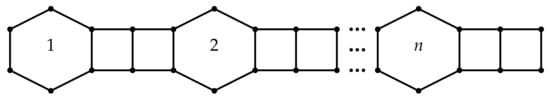
Figure 1. The graph $L_n^{6,4,4}$.

Note that ${\mathcal{L}}_{V_{12}}\left({\mathbb{L}}_n\right)={\mathcal{L}}_{V_{21}}\left({\mathbb{L}}_n\right)$ and ${\mathcal{L}}_{V_{11}}\left({\mathbb{L}}_n\right)={\mathcal{L}}_{V_{22}}\left({\mathbb{L}}_n\right).$

Let

$$T=\left(\begin{array}{cc}\frac{1}{\sqrt{2}}{I}_{4n+1}& \frac{1}{\sqrt{2}}{I}_{4n+1}\\ \frac{1}{\sqrt{2}}{I}_{4n+1}& -\frac{1}{\sqrt{2}}{I}_{4n+1}\end{array}\right).$$

Then

$$T\mathcal{L}\left({\mathbb{L}}_n\right)T^{\prime }=\left(\begin{array}{cc}{\mathcal{L}}_A& 0\\ 0& {\mathcal{L}}_S\end{array}\right).$$

$${\mathcal{L}}_A\left({\mathbb{L}}_n\right)={\mathcal{L}}_{V_{11}}+{\mathcal{L}}_{V_{12}}and{\mathcal{L}}_S\left({\mathbb{L}}_n\right)={\mathcal{L}}_{V_{11}}-{\mathcal{L}}_{V_{12}}.$$

(3)

The following lemmas are required to proceed in the future.

Lemma 1

(see [9]). Assume that G is a graph and let ${\mathcal{L}}_A$, ${\mathcal{L}}_S$ be described above. Then we have, $\Psi \left(\mathcal{L}\left(G\right)\right)=\Psi \left({\mathcal{L}}_A\left(G\right)\right)·\Psi \left({\mathcal{L}}_S\left(G\right)\right).$

Lemma 2

(see [8]). Assume that G is an n vertex graph having size m, then $K{f}^{*}\left(G\right)=2m{\displaystyle \sum _{i=2}^n}\frac{1}{{\mu }_i}.$

Lemma 3

(see [7]). Assume that G is a connected graph having size m, then $\tau \left(G\right)=\frac{1}{2m}{\displaystyle \prod _{i=1}^n}$ $d_i{\displaystyle \prod _{k=2}^n}{\mu }_k,$ where $\tau \left(G\right)$ is spanning tree.

3. Main Results

In this section, the normalized Laplacian eigenvalues of ${\mathbb{L}}_n$ are first obtained. Next, we resolve to discover the calculation for multiplicative degree-Kirchhoff index (or spanning tree) of ${\mathbb{L}}_n$. Given a square matrix A with order n, we will write to $A\left[\{i_1,i_2,\dots ,i_k\}\right]$ as the submatrix generated by eliminating the $i_{1}th,i_{2}th,\dots ,i_{k}th$ columns and rows of A. According to Equation $\left(3\right),$ the block matrices could be represented as follows.

$${\mathcal{L}}_{V_{11}}\left({\mathbb{L}}_n\right)={\left(\begin{array}{cccccccc}1& -\frac{1}{2}& 0& 0& 0& \cdots & 0& 0\\ -\frac{1}{2}& 1& -\frac{1}{\sqrt{6}}& 0& 0& \cdots & 0& 0\\ 0& -\frac{1}{\sqrt{6}}& 1& -\frac{1}{3}& 0& \cdots & 0& 0\\ 0& 0& -\frac{1}{3}& 1& -\frac{1}{3}& \cdots & 0& 0\\ 0& 0& 0& -\frac{1}{3}& 1& \cdots & 0& 0\\ ⋮& ⋮& ⋮& ⋮& ⋮& \ddots & ⋮& ⋮\\ 0& 0& 0& 0& 0& \cdots & 1& -\frac{1}{\sqrt{6}}\\ 0& 0& 0& 0& 0& \cdots & -\frac{1}{\sqrt{6}}& 1\end{array}\right)}_{(4n+1)\times (4n+1)}$$

and ${\mathcal{L}}_S\left({\mathbb{L}}_n\right)=diag\left(-\frac{1}{2},0,-\frac{1}{3},-\frac{1}{3},-\frac{1}{3},\dots ,-\frac{1}{3},-\frac{1}{2}\right)$, a diagonal matrix of order $4n+1$.

Hence,

$${\mathcal{L}}_A\left({\mathbb{L}}_n\right)={\left(\begin{array}{cccccccc}\frac{1}{2}& -\frac{1}{2}& 0& 0& 0& \cdots & 0& 0\\ -\frac{1}{2}& 1& -\frac{1}{\sqrt{6}}& 0& 0& \cdots & 0& 0\\ 0& -\frac{1}{\sqrt{6}}& \frac{2}{3}& -\frac{1}{3}& 0& \cdots & 0& 0\\ 0& 0& -\frac{1}{3}& \frac{2}{3}& -\frac{1}{3}& \cdots & 0& 0\\ 0& 0& 0& -\frac{1}{3}& \frac{2}{3}& \cdots & 0& 0\\ ⋮& ⋮& ⋮& ⋮& ⋮& \ddots & ⋮& ⋮\\ 0& 0& 0& 0& 0& \cdots & \frac{2}{3}& -\frac{1}{\sqrt{6}}\\ 0& 0& 0& 0& 0& \cdots & -\frac{1}{\sqrt{6}}& \frac{1}{2}\end{array}\right)}_{(4n+1)\times (4n+1)}$$

and

$${\mathcal{L}}_S\left({\mathbb{L}}_n\right)={\left(\begin{array}{cccccccc}\frac{3}{2}& -\frac{1}{2}& 0& 0& 0& \cdots & 0& 0\\ -\frac{1}{2}& 1& -\frac{1}{\sqrt{6}}& 0& 0& \cdots & 0& 0\\ 0& -\frac{1}{\sqrt{6}}& \frac{4}{3}& -\frac{1}{3}& 0& \cdots & 0& 0\\ 0& 0& -\frac{1}{3}& \frac{4}{3}& -\frac{1}{3}& \cdots & 0& 0\\ 0& 0& 0& -\frac{1}{3}& \frac{4}{3}& \cdots & 0& 0\\ ⋮& ⋮& ⋮& ⋮& ⋮& \ddots & ⋮& ⋮\\ 0& 0& 0& 0& 0& \cdots & \frac{4}{3}& -\frac{1}{\sqrt{6}}\\ 0& 0& 0& 0& 0& \cdots & -\frac{1}{\sqrt{6}}& \frac{3}{2}\end{array}\right)}_{(4n+1)\times (4n+1)}.$$

Assume that the eigenvalues of ${\mathcal{L}}_A\left({\mathbb{L}}_n\right)$ and ${\mathcal{L}}_S\left({\mathbb{L}}_n\right),$ are respectively, represented as ${\alpha }_i$$(i=1,2,\dots ,4n+1)$ and ${\beta }_j$$(j=1,2,\dots ,4n+1)$. According to Lemma 1 the spectrum of ${\mathbb{L}}_n$ is $\{{\alpha }_1,{\alpha }_2,\dots ,{\alpha }_{4n+1},{\beta }_1,{\beta }_2,\dots ,{\beta }_{4n+1}\}$ and it is simple to see that ${\alpha }_1=0,$${\alpha }_i>2,$$(i=2,3,\dots ,4n+1)$ and ${\beta }_j>0$$(j=1,2,\dots ,4n+1).$

Hence, we have the lemma below.

Lemma 4.

Suppose that $L_n^{6,4,4}$ be the generalized phenylenes $2n$ squares and n hexagons. Then

$$K{f}^{*}\left(L_n^{6,4,4}\right)=2(11n+1)\left[{\displaystyle \sum _{i=2}^{4n+1}}\frac{1}{{\alpha }_i}+{\displaystyle \sum _{j=1}^{4n+1}}\frac{1}{{\beta }_j}\right],$$

(4)

where ${\alpha }_i$, $(i=2,3,\dots ,4n+1)$ $({\alpha }_i>2)$ and ${\beta }_i$, $(i=1,2,\dots ,4n+1)$ are eigenvalues of ${\mathcal{L}}_A$ and ${\mathcal{L}}_S$, respectively.

According to the relationship between the coefficients and roots of $\Psi \left({\mathcal{L}}_A\right)$ (respectively. $\Psi \left({\mathcal{L}}_S\right)$), standard formulae of ${\sum }_{i=2}^{4n+1}\frac{1}{{\alpha }_i}$ (respectively. ${\sum }_{j=1}^{4n+1}\frac{1}{{\beta }_j}$) are given in the next lemmas.

Lemma 5.

Suppose that $0={\alpha }_1<{\alpha }_2\le \cdots \le {\alpha }_{4n+1}$ to be described as above. Then

$${\displaystyle \sum _{i=2}^{4n+1}}\frac{1}{{\alpha }_i}=\frac{242n^3+66n^2+13n}{33n+3}.$$

Proof. 

Suppose that $\Psi \left({\mathcal{L}}_A\right)=x^{4n+1}+a_1{x}^{4n}+\cdots +a_{4n-1}{x}^2+a_{4n}x.$ Then ${\alpha }_2,{\alpha }_3,\dots ,{\alpha }_{4n+1}$ are roots satisfies the equation below:

$$x^{4n}+a_1{x}^{4n-1}+\cdots +a_{4n-1}x+a_{4n}=0.$$

and so $\frac{1}{{\alpha }_2},\frac{1}{{\alpha }_3},\dots ,\frac{1}{{\alpha }_{4n+1}}$ are roots satisfies the equation below:

$$a_{4n}{x}^{4n}+a_{4n-1}{x}^{4n-1}+\cdots +a_{1}x+1=0.$$

Hence, by Vieta’s theorem (see [31], p. 81), we obtain

$${\displaystyle \sum _{i=2}^{4n+1}}\frac{1}{{\alpha }_i}=\frac{{(-1)}^{4n-1}{a}_{4n-1}}{{(-1)}^{4n}{a}_{4n}}.$$

(5)

For the sake of convenience, we take $S_i$ to the i-th order principal sub-matrix of ${\mathcal{L}}_A$, yield by the first $ith$ columns and rows, $i=1,2,\dots ,4n$. Let $s_i=det{S}_i$. Then

$$s_1=\frac{1}{2},s_2=\frac{1}{4},s_3=\frac{1}{12},s_4=\frac{1}{36},s_5=\frac{1}{108},s_6=\frac{1}{216},s_7=\frac{1}{648},s_8=\frac{1}{1944}$$

and

$$\left\{\begin{array}{cc}{s}_{4i}=\frac{2}{3}{s}_{4i-1}-\frac{1}{9}{s}_{4i-2},\hfill & for1\le i\le n;\hfill \\ s_{4i+1}=\frac{2}{3}{s}_{4i}-\frac{1}{9}{s}_{4i-1},\hfill & for0\le i\le n-1;\hfill \\ s_{4i+2}=s_{4i+1}-\frac{1}{6}{s}_{4i},\hfill & for0\le i\le n-1;\hfill \\ s_{4i+3}=\frac{2}{3}{s}_{4i+2}-\frac{1}{6}{s}_{4i+1},\hfill & for0\le i\le n-1.\hfill \end{array}\right.$$

These formulas in general form could be derived by a straightforward calculation as shown below.

Case 1. Suppose $s_{4i}$, $s_{4i+1}$, $s_{4i+2}$ and $s_{4i+3}$ are defined as above. We have

$$\left\{\begin{array}{cc}{s}_{4i}=\frac{3}{2}{\left(\frac{1}{54}\right)}^i,\hfill & for1\le i\le n;\hfill \\ s_{4i+1}=\frac{1}{2}{\left(\frac{1}{54}\right)}^i,\hfill & for0\le i\le n-1;\hfill \\ s_{4i+2}=\frac{1}{4}{\left(\frac{1}{54}\right)}^i,\hfill & for0\le i\le n-1;\hfill \\ s_{4i+3}=\frac{1}{12}{\left(\frac{1}{54}\right)}^i,\hfill & for0\le i\le n-1.\hfill \end{array}\right.$$

In contrast, we take $T_i$ to the i-th order principal sub-matrix of ${\mathcal{L}}_A$, built into the last $ith$ columns and rows, $i=1,2,\dots ,4n$. Let $t_i=det{T}_i$. Then

$$t_1=\frac{1}{2},t_2=\frac{1}{6},t_3=\frac{1}{18},t_4=\frac{1}{36},t_5=\frac{1}{108},t_6=\frac{1}{324},t_7=\frac{1}{972},t_8=\frac{1}{1944}$$

and

$$\left\{\begin{array}{cc}{t}_{4i}=t_{4i-1}-\frac{1}{6}{t}_{4i-2},\hfill & for1\le i\le n;\hfill \\ t_{4i+1}=\frac{2}{3}{t}_{4i}-\frac{1}{6}{t}_{4i-1},\hfill & for0\le i\le n-1;\hfill \\ t_{4i+2}=\frac{2}{3}{t}_{4i+1}-\frac{1}{9}{t}_{4i},\hfill & for0\le i\le n-1;\hfill \\ t_{4i+3}=\frac{2}{3}{t}_{4i+2}-\frac{1}{9}{t}_{4i+1},\hfill & for0\le i\le n-1.\hfill \end{array}\right.$$

These formulas in general form could be derived by a straightforward calculation as shown below.

Case 2. Suppose $t_{4i}$, $t_{4i+1}$, $t_{4i+2}$ and $t_{4i+3}$ are defined as above. We have

$$\left\{\begin{array}{cc}{t}_{4i}=\frac{3}{2}{\left(\frac{1}{54}\right)}^i,\hfill & for1\le i\le n;\hfill \\ t_{4i+1}=\frac{1}{2}{\left(\frac{1}{54}\right)}^i,\hfill & for0\le i\le n-1;\hfill \\ t_{4i+2}=\frac{1}{6}{\left(\frac{1}{54}\right)}^i,\hfill & for0\le i\le n-1;\hfill \\ t_{4i+3}=\frac{1}{18}{\left(\frac{1}{54}\right)}^i,\hfill & for0\le i\le n-1.\hfill \end{array}\right.$$

When case 1 and case 2 are combined, the following fact can be deduced.

Fact 1.${(-1)}^{4n}{a}_{4n}=\frac{11n+1}{72}{\left(\frac{1}{54}\right)}^{n-1}.$

Proof of Fact 1. The diagonal entries of ${\mathcal{L}}_A$ are denoted by $l_{ii}$. Due to the ${(-1)}^{4n}{a}_{4n}$ is a total of all principal minors of ${\mathcal{L}}_A$ with $4n$ rows and columns, we have

$${(-1)}^{4n}{a}_{4n}={\displaystyle \sum _{i=1}^{4n+1}}det{\mathcal{L}}_A\left[i\right]={\displaystyle \sum _{i=1}^{4n+1}}det\left(\begin{array}{cc}{S}_{i-1}& 0\\ 0& T\end{array}\right)={\displaystyle \sum _{i=1}^{4n+1}}det{S}_{i-1}detT,$$

(6)

where

$$T=\left(\begin{array}{cccc}{k}_{i+1,i+1}& \cdots & 0& 0\\ ⋮& \ddots & ⋮& ⋮\\ 0& \cdots & k_{4n,4n}& -\frac{1}{\sqrt{6}}\\ 0& \cdots & -\frac{1}{\sqrt{6}}& k_{4n+1,4n+1}\end{array}\right).$$

Combining Case 1, Case 2 and Equation (6), we find

$$\begin{array}{cc}\hfill {(-1)}^{4n}{a}_{4n}& ={\displaystyle \sum _{i=1}^{4n+1}}det{\mathcal{L}}_A\left[i\right]={\displaystyle \sum _{k=1}^n}det{\mathcal{L}}_A\left[4k\right]+{\displaystyle \sum _{k=1}^{n-1}}det{\mathcal{L}}_A[4k+1]\hfill \\ \hfill & +{\displaystyle \sum _{k=0}^{n-1}}det{\mathcal{L}}_A[4k+2]+{\displaystyle \sum _{k=0}^{n-1}}det{\mathcal{L}}_A[4k+3]+s_{4k}+t_{4k}\hfill \\ \hfill & ={\displaystyle \sum _{k=1}^n}{s}_{4(k-1)+3}{t}_{4(n-k)+1}+{\displaystyle \sum _{k=1}^{n-1}}{s}_{4k}{t}_{4(n-k)}+{\displaystyle \sum _{k=0}^{n-1}}{s}_{4k+1}{t}_{4(n-k-1)+3}\hfill \\ \hfill & +{\displaystyle \sum _{k=0}^{n-1}}{s}_{4k+2}{t}_{4(n-k-1)+2}+s_{4n}+t_{4n}\hfill \\ \hfill & =\frac{11n+1}{72}{\left(\frac{1}{54}\right)}^{n-1}.\hfill \end{array}$$

as desired.

Fact 2.${(-1)}^{4n-1}{a}_{4n-1}=\frac{242n^3+66n^2+13n}{216}{\left(\frac{1}{54}\right)}^{n-1}$.

Proof of Fact 2. Due to the ${(-1)}^{4n-1}{a}_{4n-1}$ is total of all principal minors of ${\mathcal{L}}_A$ with $3n-1$ rows and columns, we have

$${(-1)}^{4n-1}{a}_{4n-1}=\left|\begin{array}{ccc}{S}_{i-1}& 0& 0\\ 0& X& 0\\ 0& 0& T\end{array}\right|,1\le i<j\le 4n+1,$$

(7)

where

$$X=\left(\begin{array}{cccc}{k}_{i+1,i+1}& -\frac{1}{\sqrt{6}}& \cdots & 0\\ -\frac{1}{\sqrt{6}}& k_{i+2,i+2}& \cdots & 0\\ ⋮& ⋮& \ddots & ⋮\\ 0& 0& \cdots & k_{j-1,j-1}\end{array}\right)andT=\left(\begin{array}{cccc}{k}_{j+1,j+1}& \cdots & 0& 0\\ ⋮& \ddots & ⋮& ⋮\\ 0& \cdots & k_{4n,4n}& -\frac{1}{\sqrt{6}}\\ 0& \cdots & -\frac{1}{\sqrt{6}}& k_{4n+1,4n+1}\end{array}\right).$$

Notice that

$${(-1)}^{4n-1}{a}_{4n-1}={\displaystyle \sum _{1\le i<j}^{4n+1}}{\mathcal{L}}_A[i,j]={\displaystyle \sum _{1\le i<j}^{4n+1}}{S}_{i-1}detXdetT={\displaystyle \sum _{1\le i<j}^{4n+1}}{s}_{i-1}{t}_{4n+1-j}detX.$$

(8)

In view of Equation (8), we know that $detX$ will change as a result of the various i and j options. Hence, we will discuss by separating the cases below.

Case 1. Let $i=4k$ and $j=4l,$ for $1\le i<j\le 4n+1.$ Therefore, $1\le k<l\le n.$ In this case, X is the square matrix of order $(4l-4k-1).$

$$detX=\left|\begin{array}{ccccccc}\frac{2}{3}& -\frac{1}{\sqrt{6}}& 0& 0& \cdots & 0& 0\\ -\frac{1}{\sqrt{6}}& 1& -\frac{1}{\sqrt{6}}& 0& \cdots & 0& 0\\ 0& -\frac{1}{\sqrt{6}}& \frac{2}{3}& -\frac{1}{3}& \cdots & 0& 0\\ 0& 0& -\frac{1}{3}& \frac{2}{3}& \cdots & 0& 0\\ ⋮& ⋮& ⋮& ⋮& \ddots & ⋮& ⋮\\ 0& 0& 0& 0& \cdots & 1& -\frac{1}{\sqrt{6}}\\ 0& 0& 0& 0& \cdots & -\frac{1}{\sqrt{6}}& \frac{2}{3}\end{array}\right|=12(l-k){\left(\frac{1}{54}\right)}^{l-k}.$$

Case 2. Let $i=4k$ and $j=4l+1,$ for $1\le i<i+1<j\le 4n+1.$ Therefore, $1\le k<l\le n.$ In this case, X is the square matrix of order $(4l-4k)$.

$$detX=\left|\begin{array}{ccccccc}\frac{2}{3}& -\frac{1}{\sqrt{6}}& 0& 0& \cdots & 0& 0\\ -\frac{1}{\sqrt{6}}& 1& -\frac{1}{\sqrt{6}}& 0& \cdots & 0& 0\\ 0& -\frac{1}{\sqrt{6}}& \frac{2}{3}& -\frac{1}{3}& \cdots & 0& 0\\ 0& 0& -\frac{1}{3}& \frac{2}{3}& \cdots & 0& 0\\ ⋮& ⋮& ⋮& ⋮& \ddots & ⋮& ⋮\\ 0& 0& 0& 0& \cdots & 1& -\frac{1}{\sqrt{6}}\\ 0& 0& 0& 0& \cdots & -\frac{1}{\sqrt{6}}& \frac{2}{3}\end{array}\right|=(4l-4k+1){\left(\frac{1}{54}\right)}^{l-k}.$$

Case 3. Let $i=4k$ and $j=4l+2,$ for $1\le i<j\le 4n+1.$ Therefore, $1\le k\le l\le n-1.$ In this case, X is the square matrix of order $(4l-4k+1)$.

$$detX=\left|\begin{array}{ccccccc}\frac{2}{3}& -\frac{1}{\sqrt{6}}& 0& 0& \cdots & 0& 0\\ -\frac{1}{\sqrt{6}}& 1& -\frac{1}{\sqrt{6}}& 0& \cdots & 0& 0\\ 0& -\frac{1}{\sqrt{6}}& \frac{2}{3}& -\frac{1}{3}& \cdots & 0& 0\\ 0& 0& -\frac{1}{3}& \frac{2}{3}& \cdots & 0& 0\\ ⋮& ⋮& ⋮& ⋮& ⋮& ⋮& ⋮\\ 0& 0& 0& 0& \cdots & \frac{2}{3}& -\frac{1}{3}\\ 0& 0& 0& 0& \cdots & -\frac{1}{3}& \frac{2}{3}\end{array}\right|=\left(\frac{4}{3}l-\frac{4}{3}k+\frac{2}{3}\right){\left(\frac{1}{54}\right)}^{l-k}.$$

Case 4. Let $i=4k$ and $j=4l+3,$ for $1\le i<j\le 4n+1.$ Therefore, $1\le k\le l\le n-1.$ In this case, X is the square matrix of order $(4l-4k+2)$.

$$detX=\left|\begin{array}{ccccccc}\frac{2}{3}& -\frac{1}{\sqrt{6}}& 0& 0& \cdots & 0& 0\\ -\frac{1}{\sqrt{6}}& 1& -\frac{1}{\sqrt{6}}& 0& \cdots & 0& 0\\ 0& -\frac{1}{\sqrt{6}}& \frac{2}{3}& -\frac{1}{3}& \cdots & 0& 0\\ 0& 0& -\frac{1}{3}& \frac{2}{3}& \cdots & 0& 0\\ ⋮& ⋮& ⋮& ⋮& ⋮& ⋮& ⋮\\ 0& 0& 0& 0& \cdots & \frac{2}{3}& -\frac{1}{3}\\ 0& 0& 0& 0& \cdots & -\frac{1}{3}& \frac{2}{3}\end{array}\right|=\left(\frac{2}{3}l-\frac{2}{3}k+\frac{1}{2}\right){\left(\frac{1}{54}\right)}^{l-k}.$$

Case 5. Let $i=4k+1$ and $j=4l,$ for $1\le i<j\le 4n+1.$ Therefore, $0\le k<l\le n.$ In this case, X is the square matrix of order $(4l-4k-2)$.

$$detX=\left|\begin{array}{ccccccc}1& -\frac{1}{\sqrt{6}}& 0& 0& \cdots & 0& 0\\ -\frac{1}{\sqrt{6}}& \frac{2}{3}& -\frac{1}{3}& 0& \cdots & 0& 0\\ 0& -\frac{1}{3}& \frac{2}{3}& -\frac{1}{3}& \cdots & 0& 0\\ 0& 0& -\frac{1}{3}& \frac{2}{3}& \cdots & 0& 0\\ ⋮& ⋮& ⋮& ⋮& \ddots & ⋮& ⋮\\ 0& 0& 0& 0& \cdots & 1& -\frac{1}{\sqrt{6}}\\ 0& 0& 0& 0& \cdots & -\frac{1}{\sqrt{6}}& \frac{2}{3}\end{array}\right|=\left(\frac{2}{3}l-\frac{2}{3}k-\frac{1}{6}\right){\left(\frac{1}{54}\right)}^{l-k-1}.$$

Case 6. Let $i=4k+1$ and $j=4l+1,$ for $1\le i<j\le 4n+1.$ Therefore, $0\le k<l\le n.$ In this case, X is the square matrix of order $(4l-4k-1)$.

$$detX=\left|\begin{array}{ccccccc}1& -\frac{1}{\sqrt{6}}& 0& 0& \cdots & 0& 0\\ -\frac{1}{\sqrt{6}}& \frac{2}{3}& -\frac{1}{3}& 0& \cdots & 0& 0\\ 0& -\frac{1}{3}& \frac{2}{3}& -\frac{1}{3}& \cdots & 0& 0\\ 0& 0& -\frac{1}{3}& \frac{2}{3}& \cdots & 0& 0\\ ⋮& ⋮& ⋮& ⋮& \ddots & ⋮& ⋮\\ 0& 0& 0& 0& \cdots & 1& -\frac{1}{\sqrt{6}}\\ 0& 0& 0& 0& \cdots & -\frac{1}{\sqrt{6}}& \frac{2}{3}\end{array}\right|=\left(\frac{2}{9}l-\frac{2}{9}k\right){\left(\frac{1}{54}\right)}^{l-k-1}.$$

Case 7. Let $i=4k+1$ and $j=4l+2,$ for $1\le i<i+1<j\le 4n+1.$ Therefore, $0\le k<l\le n-1.$ In this case, X is the square matrix of order $(4l-4k)$.

$$detX=\left|\begin{array}{ccccccc}1& -\frac{1}{\sqrt{6}}& 0& 0& \cdots & 0& 0\\ -\frac{1}{\sqrt{6}}& \frac{2}{3}& -\frac{1}{3}& 0& \cdots & 0& 0\\ 0& -\frac{1}{3}& \frac{2}{3}& -\frac{1}{3}& \cdots & 0& 0\\ 0& 0& -\frac{1}{3}& \frac{2}{3}& \cdots & 0& 0\\ ⋮& ⋮& ⋮& ⋮& \ddots & ⋮& ⋮\\ 0& 0& 0& 0& \cdots & \frac{2}{3}& -\frac{1}{3}\\ 0& 0& 0& 0& \cdots & -\frac{1}{3}& \frac{2}{3}\end{array}\right|=(4l-4k+1){\left(\frac{1}{54}\right)}^{l-k}.$$

Case 8. Let $i=4k+1$ and $j=4l+3,$ for $1\le i<i+1<j\le 4n+1.$ Therefore, $0\le k<l\le n-1.$ In this case, X is the square matrix of order $(4l-4k+1)$.

$$detX=\left|\begin{array}{ccccccc}1& -\frac{1}{\sqrt{6}}& 0& 0& \cdots & 0& 0\\ -\frac{1}{\sqrt{6}}& \frac{2}{3}& -\frac{1}{3}& 0& \cdots & 0& 0\\ 0& -\frac{1}{3}& \frac{2}{3}& -\frac{1}{3}& \cdots & 0& 0\\ 0& 0& -\frac{1}{3}& \frac{2}{3}& \cdots & 0& 0\\ ⋮& ⋮& ⋮& ⋮& \ddots & ⋮& ⋮\\ 0& 0& 0& 0& \cdots & \frac{2}{3}& -\frac{1}{3}\\ 0& 0& 0& 0& \cdots & -\frac{1}{3}& \frac{2}{3}\end{array}\right|=(2l-2k+1){\left(\frac{1}{54}\right)}^{l-k}.$$

Case 9. Let $i=4k+2$ and $j=4l,$ for $1\le i<i+1<j\le 4n+1.$ Therefore, $0\le k<k+1<l\le n.$ In this case, X is the square matrix of order $(4l-4k-3)$.

$$detX=\left|\begin{array}{ccccccc}\frac{2}{3}& -\frac{1}{3}& 0& 0& \cdots & 0& 0\\ -\frac{1}{3}& \frac{2}{3}& -\frac{1}{3}& 0& \cdots & 0& 0\\ 0& -\frac{1}{3}& \frac{2}{3}& -\frac{1}{\sqrt{6}}& \cdots & 0& 0\\ 0& 0& -\frac{1}{\sqrt{6}}& 1& \cdots & 0& 0\\ ⋮& ⋮& ⋮& ⋮& \ddots & ⋮& ⋮\\ 0& 0& 0& 0& \cdots & 1& -\frac{1}{\sqrt{6}}\\ 0& 0& 0& 0& \cdots & -\frac{1}{\sqrt{6}}& \frac{2}{3}\end{array}\right|=\left(\frac{4}{3}l-\frac{4}{3}k-\frac{2}{3}\right){\left(\frac{1}{54}\right)}^{l-k-1}.$$

Case 10. Let $i=4k+2$ and $j=4l+1,$ for $1\le i<j\le 4n+1.$ Therefore, $0\le k<l\le n.$ In this case, X is the square matrix of order $(4l-4k-2)$.

$$detX=\left|\begin{array}{ccccccc}\frac{2}{3}& -\frac{1}{3}& 0& 0& \cdots & 0& 0\\ -\frac{1}{3}& \frac{2}{3}& -\frac{1}{3}& 0& \cdots & 0& 0\\ 0& -\frac{1}{3}& \frac{2}{3}& -\frac{1}{\sqrt{6}}& \cdots & 0& 0\\ 0& 0& -\frac{1}{\sqrt{6}}& 1& \cdots & 0& 0\\ ⋮& ⋮& ⋮& ⋮& \ddots & ⋮& ⋮\\ 0& 0& 0& 0& \cdots & 1& -\frac{1}{\sqrt{6}}\\ 0& 0& 0& 0& \cdots & -\frac{1}{\sqrt{6}}& \frac{2}{3}\end{array}\right|=\left(\frac{4}{9}l-\frac{4}{9}k-\frac{1}{9}\right){\left(\frac{1}{54}\right)}^{l-k-1}.$$

Case 11. Let $i=4k+2$ and $j=4l+2,$ for $1\le i<j\le 4n+1.$ Therefore, $0\le k<l\le n-1.$ In this case, X is the square matrix of order $(4l-4k-1)$.

$$detX=\left|\begin{array}{ccccccc}\frac{2}{3}& -\frac{1}{3}& 0& 0& \cdots & 0& 0\\ -\frac{1}{3}& \frac{2}{3}& -\frac{1}{3}& 0& \cdots & 0& 0\\ 0& -\frac{1}{3}& \frac{2}{3}& -\frac{1}{\sqrt{6}}& \cdots & 0& 0\\ 0& 0& -\frac{1}{\sqrt{6}}& 1& \cdots & 0& 0\\ ⋮& ⋮& ⋮& ⋮& \ddots & ⋮& ⋮\\ 0& 0& 0& 0& \cdots & \frac{2}{3}& -\frac{1}{3}\\ 0& 0& 0& 0& \cdots & -\frac{1}{3}& \frac{2}{3}\end{array}\right|=8(l-k){\left(\frac{1}{54}\right)}^{l-k}.$$

Case 12. Let $i=4k+2$ and $j=4l+3,$ for $1\le i<j\le 4n+1.$ Therefore, $0\le k<l\le n-1.$ In this case, X is the square matrix of order $(4l-4k)$.

$$detX=\left|\begin{array}{ccccccc}\frac{2}{3}& -\frac{1}{3}& 0& 0& \cdots & 0& 0\\ -\frac{1}{3}& \frac{2}{3}& -\frac{1}{3}& 0& \cdots & 0& 0\\ 0& -\frac{1}{3}& \frac{2}{3}& -\frac{1}{\sqrt{6}}& \cdots & 0& 0\\ 0& 0& -\frac{1}{\sqrt{6}}& 1& \cdots & 0& 0\\ ⋮& ⋮& ⋮& ⋮& \ddots & ⋮& ⋮\\ 0& 0& 0& 0& \cdots & \frac{2}{3}& -\frac{1}{3}\\ 0& 0& 0& 0& \cdots & -\frac{1}{3}& \frac{2}{3}\end{array}\right|=(4l-4k+1){\left(\frac{1}{54}\right)}^{l-k}.$$

Case 13. Let $i=4k+3$ and $j=4l,$ for $1\le i<i+1<j\le 4n+1.$ Therefore, $0\le k<k+1<l\le n.$ In this case, X is the square matrix of order $(4l-4k-4)$.

$$detX=\left|\begin{array}{ccccccc}\frac{2}{3}& -\frac{1}{3}& 0& 0& \cdots & 0& 0\\ -\frac{1}{3}& \frac{2}{3}& -\frac{1}{\sqrt{6}}& 0& \cdots & 0& 0\\ 0& -\frac{1}{\sqrt{6}}& 1& -\frac{1}{\sqrt{6}}& \cdots & 0& 0\\ 0& 0& -\frac{1}{\sqrt{6}}& \frac{2}{3}& \cdots & 0& 0\\ ⋮& ⋮& ⋮& ⋮& \ddots & ⋮& ⋮\\ 0& 0& 0& 0& \cdots & 1& -\frac{1}{\sqrt{6}}\\ 0& 0& 0& 0& \cdots & -\frac{1}{\sqrt{6}}& \frac{2}{3}\end{array}\right|=(4l-4k-3){\left(\frac{1}{54}\right)}^{l-k-1}.$$

Case 14. Let $i=4k+3$ and $j=4l+1,$ for $1\le i<j\le 4n+1.$ Therefore, $0\le k<l\le n.$ In this case, X is the square matrix of order $(4l-4k-3)$.

$$detX=\left|\begin{array}{ccccccc}\frac{2}{3}& -\frac{1}{3}& 0& 0& \cdots & 0& 0\\ -\frac{1}{3}& \frac{2}{3}& -\frac{1}{\sqrt{6}}& 0& \cdots & 0& 0\\ 0& -\frac{1}{\sqrt{6}}& 1& -\frac{1}{\sqrt{6}}& \cdots & 0& 0\\ 0& 0& -\frac{1}{\sqrt{6}}& \frac{2}{3}& \cdots & 0& 0\\ ⋮& ⋮& ⋮& ⋮& \ddots & ⋮& ⋮\\ 0& 0& 0& 0& \cdots & 1& -\frac{1}{\sqrt{6}}\\ 0& 0& 0& 0& \cdots & -\frac{1}{\sqrt{6}}& \frac{2}{3}\end{array}\right|=\left(\frac{4}{3}l-\frac{4}{3}k-\frac{2}{3}\right){\left(\frac{1}{54}\right)}^{l-k-1}.$$

Case 15. Let $i=4k+3$ and $j=4l+2,$ for $1\le i<j\le 4n+1.$ Therefore, $0\le k<l\le n-1.$ In this case, X is the square matrix of order $(4l-4k-2)$.

$$detX=\left|\begin{array}{ccccccc}\frac{2}{3}& -\frac{1}{3}& 0& 0& \cdots & 0& 0\\ -\frac{1}{3}& \frac{2}{3}& -\frac{1}{\sqrt{6}}& 0& \cdots & 0& 0\\ 0& -\frac{1}{\sqrt{6}}& 1& -\frac{1}{\sqrt{6}}& \cdots & 0& 0\\ 0& 0& -\frac{1}{\sqrt{6}}& \frac{2}{3}& \cdots & 0& 0\\ ⋮& ⋮& ⋮& ⋮& \ddots & ⋮& ⋮\\ 0& 0& 0& 0& \cdots & \frac{2}{3}& -\frac{1}{3}\\ 0& 0& 0& 0& \cdots & -\frac{1}{3}& \frac{2}{3}\end{array}\right|=\left(\frac{4}{9}l-\frac{4}{9}k-\frac{1}{9}\right){\left(\frac{1}{54}\right)}^{l-k-1}.$$

Case 16. Let $i=4k+3$ and $j=4l+3,$ for $1\le i<j\le 4n+1.$ Therefore, $0\le k<l\le n-1.$ In this case, X is the square matrix of order $(4l-4k-1)$.

$$detX=\left|\begin{array}{ccccccc}\frac{2}{3}& -\frac{1}{3}& 0& 0& \cdots & 0& 0\\ -\frac{1}{3}& \frac{2}{3}& -\frac{1}{\sqrt{6}}& 0& \cdots & 0& 0\\ 0& -\frac{1}{\sqrt{6}}& 1& -\frac{1}{\sqrt{6}}& \cdots & 0& 0\\ 0& 0& -\frac{1}{\sqrt{6}}& \frac{2}{3}& \cdots & 0& 0\\ ⋮& ⋮& ⋮& ⋮& \ddots & ⋮& ⋮\\ 0& 0& 0& 0& \cdots & \frac{2}{3}& -\frac{1}{3}\\ 0& 0& 0& 0& \cdots & -\frac{1}{3}& \frac{2}{3}\end{array}\right|=\left(\frac{2}{9}l-\frac{2}{9}k\right){\left(\frac{1}{54}\right)}^{l-k-1}.$$

If Equation (8) and Cases 1–16 are combined, we have

$$\begin{array}{cc}\hfill {(-1)}^{4n-1}{a}_{4n-1}& =\sum _{1\le i<j\le 4n+1}{s}_{i-1}{t}_{4n+1-j}·det{X}_{j-1-i}\hfill \\ \hfill & ={\xi }_1+{\xi }_2+{\xi }_3+{\xi }_4,\hfill \end{array}$$

(9)

where

$$\begin{array}{cc}\hfill {\xi }_1=& \sum _{1\le k<l\le n}det{\mathcal{L}}_A[4k,4l]+\sum _{1\le k\le l\le n-1}det{\mathcal{L}}_A[4k,4l+1]+\sum _{1\le k\le l\le n-1}det{\mathcal{L}}_A[4k,4l+2]\hfill \\ \hfill & +\sum _{1\le k\le l\le n-1}det{\mathcal{L}}_A[4k,4l+3]+\sum _{1\le k\le n}det{\mathcal{L}}_A[4k,4n+1]\hfill \\ \hfill & =\frac{n\left(n^2-1\right)}{12}{\left(\frac{1}{54}\right)}^{n-1}+\frac{n\left(n-1\right)\left(4n-5\right)}{48}{\left(\frac{1}{54}\right)}^{n-1}+\frac{n\left(n-1\right)\left(2n-1\right)}{36}{\left(\frac{1}{54}\right)}^{n-1}\hfill \\ \hfill & +\frac{n\left(n-1\right)\left(4n+1\right)}{48}{\left(\frac{1}{54}\right)}^{n-1}+\frac{n\left(2n-1\right)}{12}{\left(\frac{1}{54}\right)}^{n-1}\hfill \\ \hfill & =\frac{11n^3-6n^2-2n}{36}{\left(\frac{1}{54}\right)}^{n-1},\hfill \end{array}$$

$$\begin{array}{cc}\hfill {\xi }_2=& \sum _{1\le k<l\le n}det{\mathcal{L}}_A[4k+1,4l]+\sum _{1\le k<l\le n-1}det{\mathcal{L}}_A[4k+1,4l+1]+\sum _{1\le k\le l\le n-1}det{\mathcal{L}}_A[4k+1,4l+2]\hfill \\ \hfill & +\sum _{1\le k\le l\le n-1}det{\mathcal{L}}_A[4k+1,4l+3]+\sum _{1\le k\le n-1}det{\mathcal{L}}_A[4k+1,4n+1]+\sum _{1\le l\le n}det{\mathcal{L}}_A[1,4l]\hfill \\ \hfill & +\sum _{1\le l\le n-1}det{\mathcal{L}}_A[1,4l+1]+\sum _{0\le l\le n-1}det{\mathcal{L}}_A[1,4l+2]+\sum _{0\le l\le n-1}det{\mathcal{L}}_A[1,4l+3]+X_{4n-1}\hfill \\ \hfill & =\frac{n\left(n-1\right)\left(4n+1\right)}{48}{\left(\frac{1}{54}\right)}^{n-1}+\frac{n\left(n-1\right)\left(n-2\right)}{12}{\left(\frac{1}{54}\right)}^{n-1}+\frac{n\left(n-1\right)\left(4n-5\right)}{72}{\left(\frac{1}{54}\right)}^{n-1}\hfill \\ \hfill & +\frac{n\left(n-1\right)\left(2n-1\right)}{24}{\left(\frac{1}{54}\right)}^{n-1}+\frac{n\left(n-1\right)}{6}{\left(\frac{1}{54}\right)}^{n-1}+\frac{n\left(2n+1\right)}{12}{\left(\frac{1}{54}\right)}^{n-1}+\frac{n\left(n-1\right)}{6}{\left(\frac{1}{54}\right)}^{n-1}\hfill \\ \hfill & +\frac{n\left(2n-1\right)}{18}{\left(\frac{1}{54}\right)}^{n-1}+\frac{n^2}{6}{\left(\frac{1}{54}\right)}^{n-1}+\frac{2n}{9}{\left(\frac{1}{54}\right)}^{n-1}\hfill \\ \hfill & =\frac{44n^3+31n^2+25n}{144}{\left(\frac{1}{54}\right)}^{n-1},\hfill \end{array}$$

$$\begin{array}{cc}\hfill {\xi }_3=& \sum _{0\le k<l\le n}det{\mathcal{L}}_A[4k+2,4l]+\sum _{0\le k<l\le n-1}det{\mathcal{L}}_A[4k+2,4l+1]+\sum _{0\le k<l\le n-1}det{\mathcal{L}}_A[4k+2,4l+2]\hfill \\ \hfill & +\sum _{0\le k<l\le n-1}det{\mathcal{L}}_A[4k+2,4l+3]+\sum _{0\le k\le n-1}det{\mathcal{L}}_A[4k+2,4n+1]\hfill \\ \hfill & =\frac{n\left(n+1\right)\left(2n+1\right)}{36}{\left(\frac{1}{54}\right)}^{n-1}+\frac{n\left(n-1\right)\left(4n+1\right)}{72}{\left(\frac{1}{54}\right)}^{n-1}+\frac{n\left(n^2-1\right)}{27}{\left(\frac{1}{54}\right)}^{n-1}\hfill \\ \hfill & +\frac{n\left(n+1\right)\left(4n-1\right)}{72}{\left(\frac{1}{54}\right)}^{n-1}+\frac{n\left(2n+1\right)}{18}{\left(\frac{1}{54}\right)}^{n-1}\hfill \\ \hfill & =\frac{22n^3+21n^2+2n}{108}{\left(\frac{1}{54}\right)}^{n-1}\hfill \end{array}$$

$$\begin{array}{cc}\hfill {\xi }_4=& \sum _{0\le k<l\le n}det{\mathcal{L}}_A[4k+3,4l]+\sum _{0\le k<l\le n-1}det{\mathcal{L}}_A[4k+3,4l+1]+\sum _{0\le k<l\le n-1}det{\mathcal{L}}_A[4k+3,4l+2]\hfill \\ \hfill & +\sum _{0\le k<l\le n-1}det{\mathcal{L}}_A[4k+3,4l+3]+\sum _{0\le k\le n-1}det{\mathcal{L}}_A[4k+3,4n+1]\hfill \\ \hfill & =\frac{n\left(n+1\right)\left(4n-1\right)}{48}{\left(\frac{1}{54}\right)}^{n-1}+\frac{n\left(n-1\right)\left(2n-1\right)}{24}{\left(\frac{1}{54}\right)}^{n-1}+\frac{n\left(n-1\right)\left(4n+1\right)}{72}{\left(\frac{1}{54}\right)}^{n-1}\hfill \\ \hfill & +\frac{n\left(n^2-1\right)}{12}{\left(\frac{1}{54}\right)}^{n-1}+\frac{n^2}{6}{\left(\frac{1}{54}\right)}^{n-1}\hfill \\ \hfill & =\frac{44n^3+9n^2-11}{144}{\left(\frac{1}{54}\right)}^{n-1}.\hfill \end{array}$$

By substituting ${\xi }_1$, ${\xi }_2,$ ${\xi }_3$ and ${\xi }_4$ into Equation (9), the Fact 3 is completed.

The required results of Lemma 5 can be obtained by combining Fact 1 and Fact 3. □

Lemma 6.

Let $0={\beta }_1<{\beta }_2\le \cdots \le {\beta }_{4n+1}$ be the eigenvalues of ${\mathcal{L}}_S$ as above. Then${\displaystyle \sum _{j=1}^{4n+1}}\frac{1}{{\beta }_j}=\frac{{\nu }_1+{\nu }_2}{840[(2408+235\sqrt{105}){\left(41+4\sqrt{105}\right)}^{n-1}+(2408-235\sqrt{105}){\left(41-4\sqrt{105}\right)}^{n-1}},$where ${\nu }_1=(1,394,820+136,133\sqrt{105}+2380n\left(3525+344\sqrt{105}\right)){(41+4\sqrt{105})}^{n-1}$ and${\nu }_2=(1,394,820-136,133\sqrt{105}+2380n\left(3525-344\sqrt{105}\right)){(41-4\sqrt{105})}^{n-1}.$

Proof. 

Suppose that $\Psi \left({\mathcal{L}}_S\right)=x^{4n+1}+b_1{x}^{4n}+\cdots +b_{4n}x+b_{4n+1}.$

So $\frac{1}{{\beta }_1},\frac{1}{{\beta }_2},\dots ,\frac{1}{{\beta }_{4n+1}}$ are roots satisfies the equation below:

$$b_{4n+1}{x}^{4n+1}+b_{4n}{x}^{4n}+\cdots +b_{1}x+1=0.$$

By Vieta’s theorem (see [31], $P81$), we find

$${\displaystyle \sum _{i=1}^{4n+1}}\frac{1}{{\beta }_i}=\frac{{(-1)}^{4n}{b}_{4n}}{{(-1)}^{4n+1}{b}_{4n+1}}=\frac{{(-1)}^{4n}{b}_{4n}}{det{\mathcal{L}}_S}.$$

(10)

In order to find $det{\mathcal{L}}_S$ and ${(-1)}^{4n}{b}_{4n}$, consider $D_i$ to the i-th order principal sub-matrix of ${\mathcal{L}}_S$, created by the first i rows and columns, $1\le i\le 4n$. Let $d_i=det{D}_i$. Then $d_1=\frac{3}{2},$$d_2=\frac{5}{4},$$d_3=\frac{17}{12}$, $d_4=\frac{7}{4},$$d_5=\frac{235}{108},$$d_6=\frac{407}{216},$$d_7=\frac{1393}{648},$$d_8=\frac{5164}{1944}$ and

$$\left\{\begin{array}{cc}{d}_{4i}=\frac{4}{3}{d}_{4i-1}-\frac{1}{9}{d}_{4i-2},\hfill & for1\le i\le n;\hfill \\ d_{4i+1}=\frac{4}{3}{d}_{4i}-\frac{1}{9}{d}_{4i-1},\hfill & for0\le i\le n-1;\hfill \\ d_{4i+2}=d_{4i+1}-\frac{1}{6}{d}_{4i},\hfill & for0\le i\le n-1;\hfill \\ d_{4i+3}=\frac{4}{3}{d}_{4i+2}-\frac{1}{6}{d}_{4i+1},\hfill & for0\le i\le n-1.\hfill \end{array}\right.$$

We have adopted similar computation as described above.

$$\left\{\begin{array}{cc}{d}_{4i}=\frac{210+11\sqrt{105}}{280}{\left(\frac{41+4\sqrt{105}}{54}\right)}^i+\frac{210-11\sqrt{105}}{280}{\left(\frac{41-4\sqrt{105}}{54}\right)}^i,\hfill & for1\le i\le n;\hfill \\ d_{4i+1}=\frac{45+4\sqrt{105}}{60}{\left(\frac{41+4\sqrt{105}}{54}\right)}^i+\frac{45-4\sqrt{105}}{60}{\left(\frac{41-4\sqrt{105}}{54}\right)}^i,\hfill & for0\le i\le n-1;\hfill \\ d_{4i+2}=\frac{1050+101\sqrt{105}}{1680}{\left(\frac{41+4\sqrt{105}}{54}\right)}^i+\frac{1050-101\sqrt{105}}{1680}{\left(\frac{41-4\sqrt{105}}{54}\right)}^i,\hfill & for0\le i\le n-1;\hfill \\ d_{4i+3}=\frac{595+58\sqrt{105}}{840}{\left(\frac{41+4\sqrt{105}}{54}\right)}^i+\frac{595-58\sqrt{105}}{840}{\left(\frac{41-4\sqrt{105}}{54}\right)}^i,\hfill & for0\le i\le n-1.\hfill \end{array}\right.$$

Fact 3.$det{\mathcal{L}}_S=\frac{2408+235\sqrt{105}}{2016}{\left(\frac{41+4\sqrt{105}}{54}\right)}^{n-1}+\frac{2408-235\sqrt{105}}{2016}{\left(\frac{41-4\sqrt{105}}{54}\right)}^{n-1}.$

Proof of Fact 3. We can achieve $det{\mathcal{L}}_S$ in relation to its last row as

$$\begin{array}{cc}\hfill det{\mathcal{L}}_S=\frac{3}{2}det{d}_{4n}& -\frac{1}{6}det{d}_{4n-1}=\frac{3}{2}\left[\frac{210+11\sqrt{105}}{280}{\left(\frac{41+4\sqrt{105}}{54}\right)}^n+\frac{210-11\sqrt{105}}{280}{\left(\frac{41-4\sqrt{105}}{54}\right)}^n\right]\hfill \\ \hfill & -\frac{1}{6}\left[\frac{595+58\sqrt{105}}{840}{\left(\frac{41+4\sqrt{105}}{54}\right)}^{n-1}+\frac{595-58\sqrt{105}}{840}{\left(\frac{41-4\sqrt{105}}{54}\right)}^{n-1}\right]\hfill \\ \hfill & =\frac{2408+235\sqrt{105}}{2016}{\left(\frac{41+4\sqrt{105}}{54}\right)}^{n-1}+\frac{2408-235\sqrt{105}}{2016}{\left(\frac{41-4\sqrt{105}}{54}\right)}^{n-1}.\hfill \end{array}$$

On the other hand, consider $H_i$ to be the i-th order principal sub-matrix of ${\mathcal{L}}_S$, created by the last i rows and columns, $1\le i\le 4n$. Let $h_i=det{H}_i$. Then $h_1=\frac{3}{2},$$h_2=\frac{11}{6},$$h_3=\frac{41}{18}$, $h_4=\frac{71}{36},$$h_5=\frac{9}{4},$$h_6=\frac{901}{324},$$h_7=\frac{3361}{972},$$h_8=\frac{5821}{1944}$ and

$$\left\{\begin{array}{cc}{h}_{4i}=h_{4i-1}-\frac{1}{6}{h}_{4i-2},\hfill & for1\le i\le n;\hfill \\ h_{4i+1}=\frac{4}{3}{h}_{4i}-\frac{1}{6}{h}_{4i-1},\hfill & for0\le i\le n-1;\hfill \\ h_{4i+2}=\frac{4}{3}{h}_{4i+1}-\frac{1}{9}{h}_{4i},\hfill & for0\le i\le n-1;\hfill \\ h_{4i+3}=\frac{4}{3}{h}_{4i+2}-\frac{1}{9}{h}_{4i+1},\hfill & for0\le i\le n-1.\hfill \end{array}\right.$$

We have adopted similar computation as described above.

$$\left\{\begin{array}{cc}{h}_{4i}=\frac{42+3\sqrt{105}}{56}{\left(\frac{41+4\sqrt{105}}{54}\right)}^i+\frac{42-3\sqrt{105}}{56}{\left(\frac{41-4\sqrt{105}}{54}\right)}^i,\hfill & for1\le i\le n;\hfill \\ h_{4i+1}=\frac{21+2\sqrt{105}}{28}{\left(\frac{41+4\sqrt{105}}{54}\right)}^i+\frac{21-2\sqrt{105}}{28}{\left(\frac{41-4\sqrt{105}}{54}\right)}^i,\hfill & for0\le i\le n-1;\hfill \\ h_{4i+2}=\frac{154+15\sqrt{105}}{168}{\left(\frac{41+4\sqrt{105}}{54}\right)}^i+\frac{154-15\sqrt{105}}{168}{\left(\frac{41-4\sqrt{105}}{54}\right)}^i,\hfill & for0\le i\le n-1;\hfill \\ h_{4i+3}=\frac{41+4\sqrt{105}}{36}{\left(\frac{41+4\sqrt{105}}{54}\right)}^i+\frac{41-4\sqrt{105}}{36}{\left(\frac{41-4\sqrt{105}}{54}\right)}^i,\hfill & for0\le i\le n-1.\hfill \end{array}\right.$$

Fact 4.

$$\begin{array}{cc}\hfill {(-1)}^{4n}{b}_{4n}=& \frac{1,394,820+136,133\sqrt{105}+2380n\left(3525+344\sqrt{105}\right)}{1,693,440}{\left(\frac{41+4\sqrt{105}}{54}\right)}^{n-1}\hfill \\ \hfill & +\frac{1,394,820-136,133\sqrt{105}+2380n\left(3525-344\sqrt{105}\right)}{1,693,440}{\left(\frac{41-4\sqrt{105}}{54}\right)}^{n-1}.\hfill \end{array}$$

Proof of Fact 4. We noticed that ${(-1)}^{4n}{b}_{4n}$ is a total of all principal minors of ${\mathcal{L}}_S$ which have $4n$ rows and columns, then

$${(-1)}^{4n}{b}_{4n}={\displaystyle \sum _{i=1}^{4n+1}}det{\mathcal{L}}_S\left[i\right]={\displaystyle \sum _{i=1}^{4n+1}}det\left(\begin{array}{cc}{D}_{i-1}& 0\\ 0& H_{4n+1-i}\end{array}\right)={\displaystyle \sum _{i=1}^{4n+1}}det{d}_{i-1}det{h}_{4n+1-i},$$

(11)

where

$$H_{4n+1-i}=\left(\begin{array}{cccc}{l}_{i+1,i+1}& \cdots & 0& 0\\ ⋮& \ddots & ⋮& ⋮\\ 0& \cdots & l_{4n,4n}& -\frac{1}{\sqrt{6}}\\ 0& \cdots & -\frac{1}{\sqrt{6}}& l_{4n+1,4n+1}\end{array}\right).$$

In line with the above Equation (10), we find

$$\begin{array}{cc}\hfill {(-1)}^{4n}{b}_{4n}=& {\displaystyle \sum _{i=1}^{4n+1}}det{\mathcal{L}}_S\left[i\right]={\displaystyle \sum _{k=1}^n}det{\mathcal{L}}_S\left[4k\right]+{\displaystyle \sum _{k=0}^{n-1}}det{\mathcal{L}}_S[4k+1]\hfill \\ \hfill & +{\displaystyle \sum _{k=0}^{n-1}}det{\mathcal{L}}_S[4k+2]+{\displaystyle \sum _{k=0}^{n-1}}det{\mathcal{L}}_S[4k+3]+d_{4n}\hfill \\ \hfill & ={\displaystyle \sum _{k=1}^n}{d}_{4(k-1)+3}{h}_{4(n-k)+1}+{\displaystyle \sum _{k=1}^{n-1}}{d}_{4k}{h}_{4(n-k)}+{\displaystyle \sum _{k=0}^{n-1}}{d}_{4k+1}{h}_{4(n-k-1)+3}\hfill \\ \hfill & +{\displaystyle \sum _{k=0}^{n-1}}{d}_{4k+2}{h}_{4(n-k-1)+2}+d_{4n}+h_{4n}.\hfill \end{array}$$

(12)

The following forms could be derived using the above equations.

$$\begin{array}{cc}\hfill {\displaystyle \sum _{k=1}^n}{d}_{4(k-1)+3}{h}_{4(n-k)+1}& =n\left[\frac{3525+344\sqrt{105}}{3360}{\left(\frac{41+4\sqrt{105}}{54}\right)}^{n-1}+\frac{3525-344\sqrt{105}}{3360}{\left(\frac{41-4\sqrt{105}}{54}\right)}^{n-1}\right]\hfill \\ \hfill & +\frac{27\sqrt{105}}{15,680}{\left(\frac{41+4\sqrt{105}}{54}\right)}^n-\frac{27\sqrt{105}}{15,680}{\left(\frac{41-4\sqrt{105}}{54}\right)}^n,\hfill \end{array}$$

(13)

$$\begin{array}{cc}\hfill {\displaystyle \sum _{k=1}^{n-1}}{d}_{4k}{h}_{4(n-k)}& =(n-1)\left[\frac{1755+156\sqrt{105}}{2240}{\left(\frac{41+4\sqrt{105}}{54}\right)}^n+\frac{1755-156\sqrt{105}}{2240}{\left(\frac{41-4\sqrt{105}}{54}\right)}^n\right]\hfill \\ \hfill & +\frac{17}{1,128,960}\sqrt{105}{\left(\frac{41+4\sqrt{105}}{54}\right)}^{n-1}-\frac{17}{1,128,960}\sqrt{105}{\left(\frac{41-4\sqrt{105}}{54}\right)}^{n-1},\hfill \end{array}$$

(14)

$$\begin{array}{cc}\hfill {\displaystyle \sum _{k=0}^{n-1}}{d}_{4k+1}{h}_{3(n-k-1)+3}& =n\left[\frac{3525+344\sqrt{105}}{2160}{\left(\frac{41+4\sqrt{105}}{54}\right)}^{n-1}+\frac{3525-344\sqrt{105}}{2160}{\left(\frac{41-4\sqrt{105}}{54}\right)}^{n-1}\right]\hfill \\ \hfill & +\frac{11}{1120}\sqrt{105}{\left(\frac{41+4\sqrt{105}}{54}\right)}^n-\frac{11}{1120}\sqrt{105}{\left(\frac{41-4\sqrt{105}}{54}\right)}^n,\hfill \end{array}$$

(15)

$$\begin{array}{cc}\hfill {\displaystyle \sum _{k=0}^{n-1}}{d}_{4k+2}{h}_{4(n-k-1)+2}& =n\left[\frac{45,825+4472\sqrt{105}}{40,320}{\left(\frac{41+4\sqrt{105}}{54}\right)}^{n-1}+\frac{45,825-4472\sqrt{105}}{40,320}{\left(\frac{41-4\sqrt{105}}{54}\right)}^{n-1}\right]\hfill \\ \hfill & +\frac{15}{12,544}\sqrt{105}{\left(\frac{41+4\sqrt{105}}{54}\right)}^n-\frac{15}{12,544}\sqrt{105}{\left(\frac{41-4\sqrt{105}}{54}\right)}^n\hfill \end{array}$$

(16)

and

$$\begin{array}{cc}\hfill d_{4n}+h_{4n}& =\frac{210+13\sqrt{105}}{140}{\left(\frac{41+4\sqrt{105}}{54}\right)}^n+\frac{210-13\sqrt{105}}{140}{\left(\frac{41-4\sqrt{105}}{54}\right)}^n.\hfill \end{array}$$

(17)

Fact 3 is derived by substituting Equations (13)–(17) into (12).

Lemma 3 follows directly from Equation $\left(10\right)$ and Facts 3 and 4. □

We can easily obtain the following theorems by combining Lemmas 4–6.

Theorem 1.

Let $L_n^{6,4,4}$ be a generalized phenylenes with n hexagons and $2n$ squares. Then

$$K{f}^{*}\left(L_n(6,4,4)\right)=2(11n+1)\left[\frac{242n^3+66n^2+13n}{33n+3}+\frac{{(-1)}^{4n}{b}_{4n}}{det{\mathcal{L}}_S}\right],$$

where

$$\begin{array}{cc}\hfill {(-1)}^{4n}{b}_{4n}=& \frac{1,394,820+136,133\sqrt{105}+2380n\left(3525+344\sqrt{105}\right)}{1,693,440}{\left(\frac{41+4\sqrt{105}}{54}\right)}^{n-1}\hfill \\ \hfill & +\frac{1,394,820-136,133\sqrt{105}+2380n\left(3525-344\sqrt{105}\right)}{1,693,440}{\left(\frac{41-4\sqrt{105}}{54}\right)}^{n-1},\hfill \end{array}$$

$det{\mathcal{L}}_S=\frac{2408+235\sqrt{105}}{2016}{\left(\frac{41+4\sqrt{105}}{54}\right)}^{n-1}+\frac{2408-235\sqrt{105}}{2016}{\left(\frac{41-4\sqrt{105}}{54}\right)}^{n-1}.$

Theorem 2.

Let $L_n^{6,4,4}$ be a generalized phenylenes with n hexagons and $2n$ squares. Then

$$\tau \left(L_n^{6,4,4}\right)=2^{n+1}·3^{3n-1}\left[\frac{2408+235\sqrt{105}}{2016}{\left(\frac{41+4\sqrt{105}}{54}\right)}^{n-1}+\frac{2408-235\sqrt{105}}{2016}{\left(\frac{41-4\sqrt{105}}{54}\right)}^{n-1}\right].$$

Proof. 

By Lemma 3, then we have ${\prod }_{i=2}^{4n+1}{\alpha }_i{\prod }_{i=1}^{4n+1}{\beta }_i{\prod }_{v\in V_{L_n^{6,4,4}}}{d}_{L_n^{6,4,4}}=2\left|E_{L_n^{6,4,4}}\right|\tau (L_n^{6,4,4})$. Noted that

$$\prod _{v\in V_{L_n^{6,4,4}}}{d}_{L_n^{6,4,4}}=2^{2n+4}·3^{6n-2},\left|E_{L_n^{6,4,4}}\right|=11n+1,$$

$${\displaystyle \prod _{i=2}^{4n+1}}{\alpha }_i=\frac{11n+1}{72}{\left(\frac{1}{54}\right)}^{n-1},$$

$${\displaystyle \prod _{i=1}^{4n+1}}{\beta }_i=\frac{2408+235\sqrt{105}}{2016}{\left(\frac{41+4\sqrt{105}}{54}\right)}^{n-1}+\frac{2408-235\sqrt{105}}{2016}{\left(\frac{41-4\sqrt{105}}{54}\right)}^{n-1}.$$

Hence, Theorem 2 immediately follows, along with Lemma 3. □

4. Conclusions

In this article, the molecular graph $L_n^{6,4,4}$ of generalized phenylene containing $2n$ squares and n hexagons is considered. According to the decomposition theorem of normalized Laplacian polynomial, we achieve expressive formulas for the degree-Kirchhoff index and spanning tree of $L_n^{6,4,4}$.

References

- Bondy, J.A.; Murty, U.S.R. Graph Theory with Applications; MCMillan: London, UK, 1976. [Google Scholar]
- Wiener, H. Structural determination of paraffin boiling points. J. Am. Chem. Soc. 1947, 69, 17–20. [Google Scholar] [CrossRef]
- Gutman, I. Selected properties of the Schultz molecular topological index. J. Chem. Inf. Comput. Sci. 1994, 34, 1087–1089. [Google Scholar] [CrossRef]
- Klein, D.J.; Randić, M. Resistance distance. J. Math. Chem. 1993, 12, 81–95. [Google Scholar] [CrossRef]
- Klein, D.J.; Ivanciuc, O. Graph cyclicity, excess conductance, and resistance deficit. J. Math. Chem. 2001, 30, 217–287. [Google Scholar] [CrossRef]
- Gutman, I.; Mohar, B. The quasi-Wiener and the Kirchhoff indices coincide. J. Chem. Inf. Comput. Sci. 1996, 36, 982–985. [Google Scholar] [CrossRef]
- Chung, F.R.K. Spectral Graph Theory; American Mathematical Society: Providence, RI, USA, 1997. [Google Scholar]
- Chen, H.Y.; Zhang, F.J. Resistance distance and the normalized Laplacian spectrum. Discrete Appl. Math. 2007, 155, 654–661. [Google Scholar] [CrossRef] [Green Version]
- Huang, J.; Li, S.C.; Li, X.C. The normalized Laplacian degree-Kirchhoff index and spanning trees of the linear polyomino chains. Appl. Math. Comput. 2016, 289, 324–334. [Google Scholar] [CrossRef]
- Zhang, H.P.; Yang, Y.J. Resistance distance and Kirchhoff index in circulant graphs. Int. J. Quantum Chem. 2007, 107, 330–339. [Google Scholar] [CrossRef]
- Li, D.Q.; Hou, Y.P. The normalized Laplacian spectrum of quadrilateral graphs and its applications. Appl. Math. Comput. 2017, 297, 180–188. [Google Scholar] [CrossRef]
- Klein, D.J.; Lukovits, I.; Gutman, I. On the definition of the hyper-Wiener index for cycle-containing structures. J. Chem. Inf. Comput. Sci. 1995, 35, 50–52. [Google Scholar] [CrossRef]
- Zhang, H.P.; Yang, Y.J.; Li, C.W. Kirchhoff index of composite graphs. Discrete Appl. Math. 2009, 157, 2918–2927. [Google Scholar] [CrossRef] [Green Version]
- Huang, J.; Li, S.C.; Sun, L.Q. The normalized Laplacians, degree-Kirchhoff index and the spanning trees of linear hexagonal chains. Discrete Appl. Math. 2016, 207, 67–79. [Google Scholar] [CrossRef]
- He, C.; Li, S.C.; Luo, W.; Sun, L. Calculating the normalized Laplacian spectrum and the number of spanning trees of linear pentagonal chains. J. Comput. Appl. Math. 2018, 344, 381–393. [Google Scholar] [CrossRef]
- Feng, L.H.; Gutman, I.; Yu, G.H. Degree Kirchhoff index of unicyclic graphs. MATCH Commun. Math. Comput. Chem. 2013, 69, 629–648. [Google Scholar]
- Li, S.C.; Wei, W.; Yu, S. On normalized Laplacians, multiplicative degree-Kirchhoff indices and spanning Trees of the linear [n]phenylenes and their dicyclobutadieno derivatives. Int. J. Quantum Chem. 2019, 119, e25863. [Google Scholar] [CrossRef]
- Liu, J.B.; Zheng, Q.; Cai, Z.Q.; Hayat, S. On the Laplacians and normalized Laplacians for graph transformation with respect to the dicyclobutadieno derivative of [n]phenylenes. Polycycl. Aromat. Compd. 2020. [Google Scholar] [CrossRef]
- Ma, X.; Bian, H. The normalized Laplacians, degree-Kirchhoff index and the spanning trees of cylinder phenylene chain. Polycycl. Aromat. Compd. 2019. [Google Scholar] [CrossRef]
- Pan, Y.G.; Li, J.P. Kirchhoff index, multiplicative degree-Kirchhoff index and spanning trees of the linear crossed hexagonal chains. Int. J. Quantum Chem. 2018, 118, e25787. [Google Scholar] [CrossRef]
- Pan, Y.; Liu, C.; Li, J. Kirchhoff indices and numbers of spanning trees of molecular graphs derived from linear crossed polyomino chain. Polycycl. Aromat. Compd. 2020, 1–8. [Google Scholar] [CrossRef]
- Palacios, J.; Renom, J.M. Another look at the degree-Kirchhoff index. Int. J. Quantum Chem. 2011, 111, 3453–3455. [Google Scholar] [CrossRef]
- Bapat, R.A.; Karimi, M.; Liu, J.B. Kirchhoff index and degree Kirchhoff index of complete multipartite graphs. Discrete Appl. Math. 2017, 232, 41–49. [Google Scholar] [CrossRef]
- Huang, J.; Li, S.C. On the normalised Laplacian spectrum, degree-Kirchhoff index and spanning trees of graphs. Bull. Aust. Math. Soc. 2015, 91, 353–367. [Google Scholar] [CrossRef]
- Zhu, Z.X.; Liu, J.B. The normalized Laplacian, degree-Kirchhoff index and the spanning tree numbers of generalized phenylenes. Discrete Appl. Math. 2019, 254, 256–267. [Google Scholar] [CrossRef]
- Gutman, I.; Klavžar, S. Relations between Wiener numbers of benzenoid hydrocarbons and phenylenes. Models Chem. 1998, 135, 45–55. [Google Scholar]
- Gutman, I. The topological indices of linear phenylenes. J. Serb. Chem. Soc. 1995, 60, 99–104. [Google Scholar]
- Pavlović, L.; Gutman, I. Wiener numbers of phenylenes: An exact result. J. Chem. Inf. Comput. Sci. 1997, 37, 355–358. [Google Scholar]
- Chen, A.L.; Zhang, F.J. Wiener index and perfect matchings in random phenylene chains. MATCH Commun. Math. Comput. Chem. 2009, 61, 623–630. [Google Scholar]
- Geng, X.; Lei, Y. On the Kirchhoff index and the number of spanning trees of linear phenylenes chain. Polycycl. Aromat. Compd. 2021. [Google Scholar] [CrossRef]
- Vinberg, E.B. A Course in Algebra; American Mathematical Society: Providence, RI, USA, 2003. [Google Scholar]
Publisher’s Note: MDPI stays neutral with regard to jurisdictional claims in published maps and institutional affiliations. |
© 2021 by the authors. Licensee MDPI, Basel, Switzerland. This article is an open access article distributed under the terms and conditions of the Creative Commons Attribution (CC BY) license (https://creativecommons.org/licenses/by/4.0/).