A Nonparametric Lack-of-Fit Test of Constant Regression in the Presence of Heteroscedastic Variances

Abstract

We consider a k-nearest neighbor-based nonparametric lack-of-fit test of constant regression in presence of heteroscedastic variances. The asymptotic distribution of the test statistic is derived under the null and local alternatives for a fixed number of nearest neighbors. Advantages of our test compared to classical methods include: (1) The response variable can be discrete or continuous regardless of whether the conditional distribution is symmetric or not and can have variations depending on the predictor. This allows our test to have broad applicability to data from many practical fields; (2) this approach does not need nonlinear regression function estimation that often affects the power for moderate sample sizes; (3) our test statistic achieves the parametric standardizing rate, which gives more power than smoothing-based nonparametric methods for moderate sample sizes. Our numerical simulation shows that the proposed test is powerful and has noticeably better performance than some well known tests when the data were generated from high frequency alternatives or binary data. The test is illustrated with an application to gene expression data and an assessment of Richards growth curve fit to COVID-19 data.

1. Introduction

Nonparametric lack-of-fit tests where the constant regression is assumed for the null hypothesis have been considered by many authors. The order selection test [1], the rank-based order selection test [2], and the Bayes sum test [3] are among the top few that are intuitive and easy to compute. A classical textbook review of extensive efforts in nonparametric lack-of-fit tests based on smoothing methods is available in Reference [4]. Hart [2] extended the order selection method of Reference [1] to rank-based test under the constant variance assumption so that the test statistic is relatively insensitive to misspecification of distributional assumptions. These two order selection tests show excellent performance under low frequency alternatives. However, they may have low power under high frequency alternatives.

In another paper, Hart proposed several new tests based on Laplace approximations to better handle the high frequency alternatives [3]. In particular, one test with overall good power is the Bayes sum test. It is a modified cusum statistic with a better use of the sample Fourier coefficients arranged in the order of increasing frequency. Two versions of approximating the critical values were given in Reference [3], one based on normally generated data, and the other based on bootstrap resampling of the residuals under the null hypothesis of constant regression. It is interesting to note that, even though the response variable may not be from the normal distribution, the normal approximation approach tends to give even higher power than the bootstrap approach. An explanation for this is that the Bayes sum test starts with the canonical model that the estimators of the Fourier coefficients are normally distributed, and here the sample Fourier coefficients are approximately normally distributed for large sample sizes. Thus, the Bayes sum test works well for large sample sizes and is more powerful than the order selection test and the rank-based order selection test.

A major motivation for the current work is that the practical data may have variances vary with the covariate, whereas the order selection (OS), rank-based order selection (ROS), and Bayes sum test were derived for homoscedastic regression problems. The scale parameter of the error term is assumed to be a constant in these three tests. Even in such a case, different estimators of the scale parameter may be used assuming either the null or alternative hypothesis is true.

To deal with the presence of heteroscedasticity for testing the no-effect null hypothesis, Chen et al. [5] proposed another test statistic in addition to bootstrapping the [6] version of the order selection test. The approximate sampling distribution of that test statistic was obtained using the wild bootstrap method. In the case of heteroscedasticity, it was shown in Reference [5] that the asymptotic distribution of the [6] version of the order selection test depends on the unknown variance function of the errors. Moreover, they showed that their statistic is more robust than that of Reference [6] to heteroscedasticity and has better level accuracy. It was further shown in Reference [5] that the wild bootstrap technique has an overall good performance in terms of level accuracy and power properties in the case of heteroscedasticity.

Other consistent nonparametric lack-of-fit tests using some smoothing techniques have been proposed (cf. References [7,8,9,10,11,12,13,14]). Some of them are difficult to compute in addition to complicated conditions that are hard to justify. All of the aforementioned methods require the response variable to be continuous.

In this paper, we consider a nonparametric lack-of-fit test of constant regression in presence of heteroscedastic variances. This test has better power for data from high frequency alternatives than the four tests reviewed above. In addition, our test can also be applied to discrete data. The test statistic is derived using the k-nearest neighbor augmentation defined through the ranks of the predictor. This idea was first proposed in Reference [15] for analysis of covariance model, and further used in Reference [16] for a diagnostic test and in Reference [17] for a test of independence between a response variable and a covariate in presence of treatments. A test statistic was defined in Reference [16] for lack-of-fit test in the present regression setting. The authors considered each distinct covariate value as a factor level. Then, they augmented the observed data to construct what they called an artificial balanced one-way ANOVA (see Section 2.1 for further description of the augmentation). This way of constructing test statistics has great potential to gain power over smoothing-based methods. However, we found that their asymptotic variance estimator of the test statistic in Reference [16] seriously underestimates the true variance for intermediate sample sizes. As a consequence, regardless of the error distribution, their test has highly inflated type I error rates when k is small and becomes very conservative when k gets large.

In this paper, we present a very different asymptotic variance formula for the test statistic. In the special case of homoscedastic variance, our derived asymptotic variance contains one more term (a function of k) than that in Reference [16]. This explains the unstable behavior of the type I error pattern of their test. On the other hand, our test has consistent type I error rates across different sample sizes and different k values, and they are very close to the nominal alpha levels.

In Section 2, we state the hypotheses and define the test statistic as a difference of two quadratic forms, both of which estimate a common quantity but one under the null hypothesis and the other under the alternatives. Then, the asymptotic distribution of the test statistic is obtained under the null and the local alternatives for a fixed number of nearest neighbors. Moreover, we consider the idea of the Least Squares Cross-Validation (LSCV) procedure of Reference [18] to estimate the number of nearest neighbors. In Section 3, we present simulation studies with data generated having symmetric normal, light-tailed uniform, heavy-tailed T, and asymmetric heteroscedastic error distributions. The numerical results show that our test has encouragingly better performance in terms of type I error and power compared to the existing tests. In addition to the simulation comparisons, we present in Section 4 an application to gene expression data from patients undergoing radical prostatectomy and an application to assess COVID-19 model fit. A summary is given in Section 5. Technical proofs are provided in Appendix A.

2. Theoretical Results

2.1. The Hypotheses and Test Statistic

Let $(X_j,Y_j)$, $j=1,\dots ,N$, be an independent and identically distributed random sample. Let $f\left(x\right)$ and $F\left(x\right)$ denote the marginal probability density function and cumulative distribution function of $X_j$, respectively. Denote Var$\left(Y_i\right|X_i=x)={\sigma }^2\left(x\right)$ and ${\epsilon }_i=Y_i-E\left(Y_i\right|X_i)$.

We wish to test the hypotheses:

$$\begin{array}{cc}& H_0:E\left(Y\right|X=x)=m_0\left(x\right),\mathrm{where} m_0(·)\mathrm{is} \mathrm{a} \mathrm{known} \mathrm{function},\\ & \mathrm{vs}.\end{array}$$

(1)

$$H_1:E\left(Y\right|X=x)=m\left(x\right),\mathrm{which} \mathrm{depends} \mathrm{on} x \mathrm{via} \mathrm{other} \mathrm{functions} \mathrm{instead} \mathrm{of} m_0(·).$$

(2)

This formulation works for both continuous and categorical response variable Y. For simplicity in the presentation, we assume that there are no duplicated observations for each value of covariate X. If there are duplicated observations, we can use the middle ranks to take care of this issue. In regression settings, the nonlinear conditional mean regression $E\left(Y\right|X)$ is often estimated through pooling observations from neighbors by one of the smoothing methods, such as loess, smoothing spline, kernel estimation, etc. For smoothing spline or kernel method, the number of observations in a window essentially needs to go to infinity as the sample size goes to infinity. The k-nearest neighbor approach is a popular method for classification, but the theory for a fixed k is very difficult for general regression. In this work, we use a fixed number of k-nearest neighbors in the data augmentation to help define a statistic for conducting a lack-of-fit test. This augmentation is done for each unique value $x_i$ of the predictor by generating a cell that contains k values of the response Y whose corresponding x values are among the k closest to $x_i$ in rank. We consider k to be an odd number for convenience so that the augmentation contains half of the (k− 1) values symmetrically on each side of $x_i$ when $x_i$ is an inner point. Let c denote an index defined by the covariate value $X_{j_1}$, where $c=j_1$ and let $\widehat{F}\left(x\right)=N^{-1}{\sum }_{j=1}^{N}I(X_j\le x)$ denote the empirical distribution of X. We make the augmentation for each cell $\left(c\right)$ by selecting $k-1$ pairs of observations whose covariate values are among the k closest to $X_{j_1}$ in rank in addition to $(X_{j_1},Y_{j_1})$. Let $C_c$ denote the set of indices for the covariate values used in the augmented cell $\left(c\right)$. Thus, for any pair $(X_j,Y_j)$ to be selected in the augmentation of the cell $\left(c\right)$, the difference between the ranks of $X_j$ and $X_{j_1}$ is no more than $(k-1)/2$ if $X_{j_1}$ is an interior point whose rank is between $(k-1)/2$ and $N-(k-1)/2$, i.e., $N|\widehat{F}\left(X_{j_1}\right)-\widehat{F}\left(X_j\right)|\le (k-1)/2$. For $X_{j_1}$ whose rank is less than $(k-1)/2$ or greater than $N-(k-1)/2$, the difference between the ranks of $X_j$ and $X_{j_1}$ is no more than $k-1$. This idea was first proposed in [15] and further used in References [16,17] for different problems. A test statistic was derived in Reference [16] for lack-of-fit testing in the present regression setting by considering each distinct covariate value as a factor level. Then, the observed data were augmented by considering a window around each $x_i$ that contains the $k_n$ nearest covariate values to construct what the authors called an artificial balanced one-way ANOVA. Similar augmentation was considered in Reference [17] when there are more than one treatment. Their results cannot be applied here since the asymptotic variance calculation is ill-defined when there is no treatment factor as in our lack-of-fit setting.

Let $R_{ct},t=1,\dots ,k$, denote the augmented response values in cell $\left(c\right)$ under the null hypothesis. Define $g_{Nk}(X_1,X_2)=I\left(N|\widehat{F}\left(X_1\right)-\widehat{F}\left(X_2\right)|\le \frac{k-1}{2}\right)$ to be the indicator function that the difference between the ranks of $X_1$ and $X_2$ is no more than $(k-1)/2$. Let $B_N$ and $W_N$ denote the average between-cell and within-cell variations defined as the following:

$$\begin{array}{c}\hfill B_N=\frac{k}{N-1}\sum _{c=1}^N{\left({\overline{R}}_{c·}-{\overline{R}}_{··}\right)}^2\mathrm{and}{W}_N=\frac{1}{N(k-1)}\sum _{c=1}^N\sum _{t=1}^k{\left(R_{ct}-{\overline{R}}_{c·}\right)}^2,\end{array}$$

where ${\overline{R}}_{c·}=k^{-1}{\sum }_{t=1}^k{R}_{ct}$, ${\overline{R}}_{··}=N^{-1}{\sum }_{c=1}^N{\overline{R}}_{c·}.$ Note that $B_N$ and $W_N$ can be easily calculated since they resemble the mean squares statistics for an ANOVA model. The calculation is on the augmented data. In most cases in the literature, $B_N/W_N$ is used for constructing the test statistic when $B_N$ has fixed degrees of freedom. However, in our case, the degrees of freedom for $B_N$ is $N-1$, which goes to infinity. Therefore, the staztistic typically used in this case is $\sqrt{N}[(B_N/W_N)-1]$ (see Reference [19]), which involves showing that $\sqrt{N}(B_N-W_N)$ converges in distribution to normality and $W_N$ converges in probability to a constant. With augumented data, it is complicated to show that $W_N$ converges in probability. So, we define the following difference-based

$$G_N=\sqrt{N}(B_N-W_N)/\sqrt{{\widehat{\lambda }}_N}$$

as our test statistic instead of using $B_N/W_N$-based one, where ${\widehat{\lambda }}_N$ is a variance estimator for $\sqrt{N}(B_N-W_N)$ given later in (9). This test statistic is similar to that proposed in Reference [16], but with a different variance estimator.

To express $B_N$ and $W_N$ in terms of the original data, we can write

$$\begin{array}{ccc}\hfill B_N& =& \frac{k}{N-1}\sum _{j_1=1}^N{\left[\frac{1}{k}\sum _{j=1}^N{Y}_j{g}_{Nk}(X_{j1},X_j)-\frac{1}{Nk}\sum _{j_2=1}^N\sum _{j=1}^N{Y}_j{g}_{Nk}(X_{j2},X_j)\right]}^2+O_p\left(N^{-1}\right),\hfill \\ \hfill W_N& =& \frac{1}{N(k-1)}\sum _{j_1=1}^N\sum _{j=1}^N{\left[Y_j{g}_{Nk}(X_{j1},X_j)-\frac{1}{k}\sum _{j_2=1}^N{Y}_{j_2}{g}_{Nk}(X_{j1},X_{j2})\right]}^2+O_p\left(N^{-1}\right).\hfill \end{array}$$

2.2. Asymptotic Distribution of the Test Statistic under the Null Hypothesis

Even though the test statistic is easy to calculate, the derivation of the asymptotic distribution is challenging since the augmented data in neighboring cells are correlated. In this subsection, we derive the asymptotic distribution of the test statistic derived with a different strategy than that proposed in Reference [16]. We first simplify it by finding its projection. Specifically, define

$$\begin{array}{c}\hfill V_{ct}=R_{ct}-E\left(R_{ct}\right|\mathbf{X}),\end{array}$$

where $\mathbf{X}={(X_1,\dots ,X_N)}^{\prime }$. Then, we project $B_N$ onto the space:

$$\begin{array}{c}\hfill \mathrm{Extended} \mathrm{span}\{{\mathbf{V}}_c,c=1,\dots ,N\}\end{array}$$

(3)

of the form ${\sum }_{c=1}^N{a}_c{g}_c\left({\mathbf{V}}_c\right)$, where $a_i$ are constants, ${\mathbf{V}}_c={(V_{c1},···,V_{ck})}^{\prime }$, and $g_c\left({\mathbf{V}}_c\right)$ is some function that is possibly nonlinear. This projection will help us to split $B_N$ into two terms, one of which includes a summation over c and the other over c and $c^{\prime }$ for $c\ne c^{\prime }$:

$$\begin{array}{c}\hfill B_N=P_B\left(\mathbf{V}\right)+S_B\left(\mathbf{V}\right),\end{array}$$

$$\begin{array}{c}\hfill P_B\left(\mathbf{V}\right)=\frac{k}{N}\sum _{c=1}^N{\overline{V}}_{c·}^2,S_B\left(\mathbf{V}\right)=\frac{-k}{N(N-1)}\sum _{c\ne c^{\prime }}^N{\overline{V}}_{c·}{\overline{V}}_{c^{\prime }·},\end{array}$$

(4)

where ${\mathbf{V}}^{\prime }=({\mathbf{V}}_1^{\prime },\dots ,{\mathbf{V}}_N^{\prime })$ and ${\overline{V}}_{c·}=k^{-1}{\sum }_{t=1}^k{V}_{ct}$. Then, $P_B\left(\mathbf{V}\right)$ is in the space defined in (3) and $B_N-W_N=(P_B\left(\mathbf{V}\right)-W_N)+S_B\left(\mathbf{V}\right)=T_B+S_B\left(\mathbf{V}\right),$ where

$$\begin{array}{ccc}\hfill T_B& =& \frac{1}{N(k-1)}\sum _{c=1}^N\sum _{t\ne t^{\prime }}^k{V}_{ct}{V}_{c{t}^{\prime }}=\frac{1}{N(k-1)}\sum _{c=1}^N\sum _{t\ne t^{\prime }}^k(R_{ct}-E\left(R_{ct}\right|\mathbf{X}))(R_{c{t}^{\prime }}-E\left(R_{c{t}^{\prime }}\right|\mathbf{X}))\hfill \\ & =& \frac{1}{N(k-1)}\sum _{j\ne j^{\prime }}^N(Y_j-E\left(Y_j\right|\mathbf{X}))(Y_{j^{\prime }}-E\left(Y_{j^{\prime }}\right|\mathbf{X}))\sum _{c=1}^{N}I(j\in C_c)I(j^{\prime }\in C_c)\hfill \\ & =& \frac{1}{N(k-1)}\sum _{j\ne j^{\prime }}^N(Y_j-E\left(Y_j\right|\mathbf{X}))(Y_{j^{\prime }}-E\left(Y_{j^{\prime }}\right|\mathbf{X}))K_{j{j}^{\prime }},\hfill \end{array}$$

(5)

and

$$\begin{array}{c}\hfill K_{j{j}^{\prime }}=\sum _{c=1}^{N}I(j\in C_c)I(j^{\prime }\in C_c).\end{array}$$

(6)

Note that the term in (5) is closely related to the expected covariance between every pair of response values with correlation induced by their dependence on $\mathbf{X}$. The $K_{j{j}^{\prime }}$ in (6) serves as a weight function which associates the response locally the empirical distribution function of X. The $T_B$ term in (5) is more intuitive than $\sqrt{N}(B_N-W_N)$ to evaluate the lack-of-fit. However, $T_B$ cannot be calculated from the sample since $E\left(Y\right|X)$ is unknown. On the other hand, $\sqrt{N}(B_N-W_N)$ can be directly obtained from the sample.

We assume the following condition to obtain the result under the null hypothesis:

Assumption 1.

For all x, suppose that $F\left(x\right)$ is differentiable, and the fourth conditional central moment of $Y_j$ given $X_j$ is uniformly bounded.

The advantage of using a small or fixed k instead of a large k can be seen here. Even though $S_B\left(\mathbf{V}\right)$ is a quadratic form, only nearby cells have correlated observations due to the fixed number of nearest neighbors augmentation. On the other hand, when the number of nearest neighbors tends to infinity, the augmented data in many more cells will be correlated; therefore, $S_B\left(\mathbf{V}\right)$ might diverge, and the derivation of the asymptotic distribution will require unnecessarily strong conditions on the magnitude of the correlation. It is straightforward to show that $S_B\left(\mathbf{V}\right)=O_P\left(N^{-1}\right)$ with a small or fixed k. Hence, $\sqrt{N}{S}_B\left(\mathbf{V}\right)$ is asymptotically negligible. We state this result in Lemma 1 below.

Lemma 1

(Projection of $B_N$). Let $S_B\left(\mathbf{V}\right)$ be as defined in (4). If the Assumption 1 is satisfied, then

$$\begin{array}{c}\hfill \sqrt{N}{S}_B\left(\mathbf{V}\right)\stackrel{p}{\to }0,asN\to \infty ,\end{array}$$

where the notation $\stackrel{p}{\to }$ denotes convergence in probability.

To obtain the asymptotic distribution of the test statistic under the null hypothesis, we work with

$$\begin{array}{c}\hfill \sqrt{N}{T}_B=\frac{\sqrt{N}}{N(k-1)}\sum _{j\ne j^{\prime }}^N(Y_j-E\left(Y_j\right|\mathbf{X}))(Y_{j^{\prime }}-E\left(Y_{j^{\prime }}\right|\mathbf{X}))K_{j{j}^{\prime }},\end{array}$$

(7)

where $K_{j{j}^{\prime }}$ is defined in (6). We first give the large sample behavior of the variance of this term.

Theorem 1.

Under Assumption 1, $\lambda :={lim}_{N\to \infty }{\lambda }_N={lim}_{N\to \infty }\mathit{Var}\left(\sqrt{N}{T}_B\right)$ exists and

$$\begin{array}{c}\hfill \lambda =E(\underset{N\to \infty }{lim}{\delta }_N),\end{array}$$

where

$$\begin{array}{cc}\hfill {\delta }_N& ={\sum }_{j<j^{\prime }}^N\frac{4{\sigma }^2\left(X_j\right){\sigma }^2\left(X_{j^{\prime }}\right)}{N{(k-1)}^2}\left[[k-|j_{*}^{\prime }-j_{*}{\left|\right]}^2+[k-|j_{*}^{\prime }-j_{*}\left|\right]\right.\\ & \left.-2I\left(|j_{*}^{\prime }-j_{*}|\le \frac{k-1}{2}\right)+O\left(N^{-1}\right)\right]I\left(\right|j_{*}^{\prime }-j_{*}|\le k-1),\end{array}$$

(8)

and $j_{*}^{\prime },j_{*}$ are the ranks of $X_{j^{\prime }}$ and $X_j$ among the covariate values $X_1,\dots ,X_N$.

To estimate the asymptotic variance, let $j_{*}$ be the rank of $X_j$ among all covariate values. Then, it is readily seen that a consistent estimator of $\lambda$ under $H_0$ is

$${\widehat{\lambda }}_N=\sum _{j<j^{\prime }}^N\frac{4{\widehat{\sigma }}^2\left(X_j\right){\widehat{\sigma }}^2\left(X_{j^{\prime }}\right)}{N{(k-1)}^2}\left[[k-|j_{*}^{\prime }-j_{*}{\left|\right]}^2+[k-|j_{*}^{\prime }-j_{*}\left|\right]-2I\left(|j_{*}^{\prime }-j_{*}|\le \frac{k-1}{2}\right)\right]I\left(\right|j_{*}^{\prime }-j_{*}|\le k-1),$$

(9)

where ${\widehat{\sigma }}^2\left(X_j\right)$ is the sample variance based on the augmented observations for the cell determined by $X_j$, i.e.,

$$\begin{array}{c}\hfill {\widehat{\sigma }}^2\left(X_j\right)=\frac{1}{k-1}\left\{\sum _{l=1}^N{Y}_l^2{g}_{Nk}(X_l,X_j)-\frac{1}{k}{\left(\sum _{l=1}^N{Y}_l{g}_{Nk}(X_l,X_j)\right)}^2\right\}.\end{array}$$

Note that $K_{j{j}^{\prime }}$ are bounded counts and (7) is a clean quadratic form as defined in Reference [20]. The Central Limit Theorem for clean quadratic forms (Proposition 3.2) in Reference [20] can be applied to obtain the following result. We omit the details of the proof.

Theorem 2.

Under $H_0$ in (1) and Assumption 1,

$$\begin{array}{c}\hfill G_N\stackrel{d}{\to }N(0,1),asN\to \infty ,\end{array}$$

where the notation $\stackrel{d}{\to }$ denotes convergence in distribution.

2.3. Results under Local or Fixed Alternatives

In this subsection, we consider the theoretical properties of the test under fixed or local alternatives in which the conditional expectation of Y given X is $m\left(x\right)=E\left(Y\right|X=x)$. Let $A\left(x\right)$ be an univariate function of x.

Under a fixed alternative, $m\left(x\right)$ can be expressed as

$$\begin{array}{c}\hfill m\left(x\right)=m_0\left(x\right)+A\left(x\right),\end{array}$$

(10)

where $m_0\left(x\right)=E_0\left(Y\right|X=x)$ is the conditional expectation of Y given X under the null hypothesis.

For local alternatives, consider the sequence of conditional expectations $E_N\left(Y\right|X=x)$ that approach $m_0\left(x\right)$ in the order of $N^{-1/4}$:

$$\begin{array}{c}\hfill m\left(x\right)=E_N\left(Y\right|X=x)=m_0\left(x\right)+N^{-1/4}A\left(x\right).\end{array}$$

(11)

Both alternatives are valid for either discrete or continuous response variable and allow the data to have different conditional variance under the alternative hypotheses from that under the null. For example, if $Y|X$ has a Poisson distribution with mean $m\left(x\right)$ under the alternative, then the variance is $m\left(x\right)$ instead of $m_0\left(x\right)$.

Suppose $(X_i,Y_i)$, $i=1,\dots ,N$ are observed data under either the fixed alternatives in (10) or the local alternatives in (11). Let $\mathbf{Q}=\{Q_{ct};c=1,\cdots ,N,t=1,\cdots ,k\}$ be the augmented response values. Note that $Q_{ct}$ is equal to the observed response variable whose covariate value is one of the following:

$$\begin{array}{c}\hfill \left\{\begin{array}{cc}{X}_{\left(t\right)}\hfill & \mathrm{if} c<(k-1)/2,\hfill \\ X_{(c+t-(k+1)/2)}\hfill & \mathrm{if} (k-1)/2\le c\le N-(k-1)/2,\hfill \\ X_{(N-k+t)}\hfill & \mathrm{if} c>N-(k-1)/2.\hfill \end{array}\right.\end{array}$$

Then, $Q_{ct}$ can be written as $Q_{ct}={\epsilon }_{ct}+E\left(Q_{ct}\right|\mathbf{X})$, where $E\left(Q_{ct}\right|\mathbf{X})$ includes the conditional mean under the null hypothesis and departure from the null. Note that ${\epsilon }_{ct}=Q_{ct}-E\left(Q_{ct}\right|\mathbf{X})$ satisfies the null hypothesis and can be viewed as the augmented data for $Z_i=Y_i-\left(m_0\left(X_i\right)+A\left(X_i\right)\right)$ if $(X_i,Y_i)$ are under the fixed alternative in (10) or for $Z_i=Y_i-\left(m_0\left(X_i\right)+N^{-1/4}A\left(X_i\right)\right)$ if $(X_i,Y_i)$ are under the local alternatives in (11). In either case, the conditional mean $Z_i$ given $X_i$ satisfies the null hypothesis but with $\mathit{Var}\left(Z_i\right|X_i)$ equal to $\mathit{Var}\left(Y_i\right|X_i)$ under the alternative hypotheses. For convenience, define $A_{ct}$ to be the $A\left(x\right)$ function evaluated at the covariate value for augmented observation $Q_{ct}$. Let ${\overline{A}}_{c·}=k^{-1}{\sum }_{t=1}^k{A}_{ct}$, ${\overline{A}}_{··}=N^{-1}{\sum }_{c=1}^N{\overline{A}}_{c·}$, ${\overline{Q}}_{c·}=k^{-1}{\sum }_{t=1}^k{Q}_{ct}$, ${\overline{Q}}_{··}=N^{-1}{\sum }_{c=1}^N{\overline{Q}}_{c·}$, ${\overline{\epsilon }}_{c·}=k^{-1}{\sum }_{t=1}^k{\epsilon }_{ct}$, and ${\overline{\epsilon }}_{··}=N^{-1}{\sum }_{c=1}^N{\overline{\epsilon }}_{c·}$. Denote $B_N\left(\mathbf{Q}\right)$ and $W_N\left(\mathbf{Q}\right)$ to be the average between-cell variations and the average within-cell variations under the alternative hypotheses, respectively.

Under the local alternatives,

$$\begin{array}{ccc}\hfill B_N\left(\mathbf{Q}\right)& =& k{(N-1)}^{-1}\sum _{c=1}^N{\left({\overline{Q}}_{c·}-{\overline{Q}}_{··}\right)}^2=k{(N-1)}^{-1}\sum _{c=1}^N{\left[\left({\overline{\epsilon }}_{c·}-{\overline{\epsilon }}_{··}\right)+N^{-1/4}\left({\overline{A}}_{c·}-{\overline{A}}_{··}\right)\right]}^2\hfill \\ & =& k{(N-1)}^{-1}\sum _{c=1}^N\left[{\left({\overline{\epsilon }}_{c·}-{\overline{\epsilon }}_{··}\right)}^2+N^{-1/2}{\left({\overline{A}}_{c·}-{\overline{A}}_{··}\right)}^2\right.+\left.2N^{-1/4}\left({\overline{A}}_{c·}-{\overline{A}}_{··}\right)\left({\overline{\epsilon }}_{c·}-{\overline{\epsilon }}_{··}\right)\right],\hfill \end{array}$$

and

$$\begin{array}{ccc}& & W_N\left(\mathbf{Q}\right)\hfill \\ & & ={\left\{N(k-1)\right\}}^{-1}\sum _{c=1}^N\sum _{t=1}^k{\left(Q_{ct}-{\overline{Q}}_{c·}\right)}^2={\left\{N(k-1)\right\}}^{-1}\sum _{c=1}^N\sum _{t=1}^k{\left[\left({\epsilon }_{ct}-{\overline{\epsilon }}_{c·}\right)+N^{-1/4}\left(A_{ct}-{\overline{A}}_{c·}\right)\right]}^2\hfill \\ & & ={\left\{N(k-1)\right\}}^{-1}\sum _{c=1}^N\sum _{t=1}^k\left[{\left({\epsilon }_{ct}-{\overline{\epsilon }}_{c·}\right)}^2+N^{-1/2}{\left(A_{ct}-{\overline{A}}_{c·}\right)}^2+2N^{-1/4}\left({\epsilon }_{ct}-{\overline{\epsilon }}_{c·}\right)\left(A_{ct}-{\overline{A}}_{c·}\right)\right].\hfill \end{array}$$

In this case, the numerator of the test statistic can be written as

$$\begin{array}{c}\hfill \sqrt{N}(B_N\left(\mathbf{Q}\right)-W_N\left(\mathbf{Q}\right))={\Delta }_{N,0}+{\Delta }_{N,1}+{\Delta }_{N,2}-{\Delta }_{N,3}-{\Delta }_{N,4},\end{array}$$

(12)

where

$$\begin{array}{ccc}\hfill {\Delta }_{N,0}& =& \sqrt{N}\left(k{(N-1)}^{-1}\sum _{c=1}^N{\left({\overline{\epsilon }}_{c·}-{\overline{\epsilon }}_{··}\right)}^2-{\left\{N(k-1)\right\}}^{-1}\sum _{c=1}^N\sum _{t=1}^k{\left({\epsilon }_{ct}-{\overline{\epsilon }}_{c·}\right)}^2\right),\hfill \end{array}$$

(13)

$$\begin{array}{ccc}\hfill {\Delta }_{N,1}& =& \sqrt{N}k{(N-1)}^{-1}\sum _{c=1}^N\left[N^{-1/2}{\left({\overline{A}}_{c·}-{\overline{A}}_{··}\right)}^2\right],\hfill \end{array}$$

(14)

$$\begin{array}{ccc}\hfill {\Delta }_{N,2}& =& \sqrt{N}k{(N-1)}^{-1}\sum _{c=1}^N\left[2N^{-1/4}\left({\overline{A}}_{c·}-{\overline{A}}_{··}\right)\left({\overline{\epsilon }}_{c·}-{\overline{\epsilon }}_{··}\right)\right],\hfill \end{array}$$

(15)

$$\begin{array}{ccc}\hfill {\Delta }_{N,3}& =& \sqrt{N}{\left\{N(k-1)\right\}}^{-1}\sum _{c=1}^N\sum _{t=1}^k\left[N^{-1/2}{\left(A_{ct}-{\overline{A}}_{c·}\right)}^2\right],\hfill \end{array}$$

(16)

$$\begin{array}{ccc}\hfill {\Delta }_{N,4}& =& 2\sqrt{N}{\left\{N(k-1)\right\}}^{-1}\sum _{c=1}^N\sum _{t=1}^k\left({\epsilon }_{ct}-{\overline{\epsilon }}_{c·}\right)N^{-1/4}\left(A_{ct}-{\overline{A}}_{c·}\right).\hfill \end{array}$$

(17)

Similarly, under the fixed alternatives,

$$\begin{array}{c}\hfill \sqrt{N}(B_N\left(\mathbf{Q}\right)-W_N\left(\mathbf{Q}\right))={\Delta }_{N,0}+\sqrt{N}{\Delta }_{N,1}+N^{\frac{1}{4}}{\Delta }_{N,2}-\sqrt{N}{\Delta }_{N,3}-N^{\frac{1}{4}}{\Delta }_{N,4},\end{array}$$

(18)

where ${\Delta }_{N,i}$, $i=0,\dots ,4$ are given in (13)–(17).

The following additional condition is needed for the result under the alternative hypotheses:

Assumption 2.

Suppose that $X_i$ has bounded support $[a,b]$, and $A\left(x\right)$ is locally Lipschitz continuous on $[a,b]$: for each $z\in [a,b]$, there exists an $L>0$ such that $A\left(x\right)$ is Lipschitz continuous on the neighborhood $B_L\left(z\right)=\{y\in [a,b]:|y-z|<L\}$. Further, we assume that the fourth central moments of $A\left(X_i\right)$ are uniformly bounded.

Before we give the asymptotic distribution of the test statistic under the alternatives, we state the following results which are valid under both the local and fixed alternative hypotheses.

Lemma 2.

Under Assumptions 1 and 2, as $N\to \infty$,

$$\begin{array}{c}\hfill \left(i\right){\Delta }_{N,2}=O_p\left(N^{-\frac{1}{4}}\right);\left(ii\right){\Delta }_{N,3}=O_p\left(N^{-2}\right);\left(iii\right){\Delta }_{N,4}=O_p\left(N^{-\frac{3}{4}}\right),\end{array}$$

where ${\Delta }_{N,2}$, ${\Delta }_{N,3}$, and ${\Delta }_{N,4}$ are defined in (15), (16), and (17), respectively.

The proof of Lemma 2 is given in Appendix A. From this Lemma and Equations (12) and (18), we can see that ${\Delta }_{N,0}$ and ${\Delta }_{N,1}$ are the major terms that provide power under the alternative hypotheses. We state the results separately for fixed and local alternatives.

Theorem 3.

Let ${\lambda }_{NA}$ be defined similarly as ${\lambda }_N$ in Theorem 1 but with ${\sigma }^2\left(X_j\right)$ calculated under the alternatives in (11). For the sequence of local alternatives $E_N\left(Y\right|X)$ in (11) and under the Assumptions 1 and 2, the limit ${\lambda }_A={lim}_{N\to \infty }{\lambda }_{NA}$ exists and

$$\begin{array}{c}\hfill G_N\stackrel{d}{\to }N(k{\sigma }_A^2/\sqrt{{\lambda }_A},1),\end{array}$$

where

$$\begin{array}{c}\hfill {\sigma }_A^2={\int }_{-\infty }^{\infty }{A}^2\left(x\right)f\left(x\right)dx-{\left({\int }_{-\infty }^{\infty }A\left(x\right)f\left(x\right)dx\right)}^2=\mathit{Var}\left(A\left(X\right)\right).\end{array}$$

(19)

Note that ${\lambda }_N$ in Theorem 1 and ${\lambda }_{NA}$ in Theorem 3 share the same formula, except that ${\sigma }^2\left(X_j\right)=\mathit{Var}\left(Y_j\right|X_j)$ in ${\lambda }_{NA}$ needs to be calculated under the alternatives in (11). For example, if Y given X has a Bernoulli distribution, then the conditional variance of Y given X under the local alternatives in (11) is ${\sigma }^2\left(x\right)=E_N\left(Y\right|X=x)(1-E_N\left(Y\right|X=x))=m\left(x\right)(1-m\left(x\right))$, which is different from that under the null hypothesis $E_0\left(Y\right|X=x)(1-E_0\left(Y\right|X=x))=m_0\left(x\right)(1-m_0\left(x\right))$.

Theorem 4.

For the fixed alternative in (10), under Assumptions 1 and 2, the power of the test using statistic $G_N$ goes to one as $N\to \infty$.

The proofs of Theorems 3 and 4 are given in Appendix A.

In heteroscedastic regression, it is common in the literature to write $Y_i=m\left(X_i\right)+\sigma \left(X_i\right)e_i$ with $e_i$ independent of $X_i$. In this formulation, the entire error term $\sigma \left(X_i\right)e_i$ is uncorrelated with $X_i$. In the ideal case that there is no lack-of-fit, such a model is reasonable. However, when there is a lack-of-fit because a wrong regression function is specified, the error term still contains some systematic information of $E\left(Y_i\right|X_i)$. Then, it is possible that the error resulting from the specified regression function is still correlated with $X_i$.

2.4. Selection of the Number of Nearest Neighbors

The number of nearest neighbors k in the test statistic specifies the number of values augmented in each cell. Our theory requires that it takes a finite small odd integer. In simulations, we have found that the type I error remains close to the nominal level for different small k values and stays stable for a broad range of sample sizes and error distributions. Under the alternative hypothesis, different k may lead to different power for our test statistic. This section discusses how to select the parameter k.

Under the alternative hypothesis, our k-nearest neighbor augmentation is parallel to regression using a local constant based on k-nearest neighbors. For a continuous response variable, Hardle et al. [18] suggested the Least Squares Cross-Validation (LSCV) method for smoothing parameter (bandwidth) selection in kernel regression estimation. Chen et al. [5] recommended using the one-sided cross-validation procedure of Reference [21] to select smoothing parameter (bandwidth) for hypothesis testing. The number of nearest neighbors k in our setting has a similar role as the smoothing parameter in kernel regression.

For a categorical response variable, Holmes et al. [22] proposed an approach to select the parameter k in the k-nearest neighbor (KNN) classification algorithm using likelihood-based inference. Choosing k in this method can be considered as a generalized linear model variable-selection problem. In particular, for multinomial data $(y_i,{\mathbf{x}}_i)$, $i=1,\dots ,n$, where $y_i\in \{C_0,\cdots ,C_Q\}$ denotes the class label of the ith observation, and ${\mathbf{x}}_i$ is a vector of p predictor variables, they considered the probability model

$$\begin{array}{c}\hfill pr(y_i=C_i|y_{[-i]},{\mathbf{x}}_i,k)=\frac{exp\left(z_i^{(k,j)}\theta \right)}{{\sum }_{\upsilon =0}^{Q}exp\left(z_i^{(k,\upsilon )}\theta \right)},\end{array}$$

where $y_{[-i]}=\{y_1,\dots ,y_{i-1},y_{i+1},\dots ,y_n\}$ denotes the data with the ith observation deleted, $\theta$ is a single regression parameter, and $z_i^{(k,\upsilon )}$ is the difference between the proportion of observations in class $C_{\upsilon }$ and that in class $C_0$ within the k-nearest neighbors of ${\mathbf{x}}_i$, i.e.,

$$\begin{array}{c}\hfill z_i^{(k,\upsilon )}=\frac{1}{k}\sum _{j\stackrel{k}{\sim }i}\{I(y_j=C_{\upsilon })-I(y_j=C_0)\},\end{array}$$

where the notation ${\sum }_{j\stackrel{k}{\sim }i}$ denotes that the summation is over the k-nearest neighbors of ${\mathbf{x}}_i$ in the set $\{{\mathbf{x}}_1,\cdots ,{\mathbf{x}}_{i-1},{\mathbf{x}}_{i+1},\cdots ,{\mathbf{x}}_n\}$, and the neighbors are defined based on the Euclidean distance. The prediction for a new point $y_{n+1}|{\mathbf{x}}_{n+1}$ is given by the most common class in the k-nearest neighbors of ${\mathbf{x}}_{n+1}$. Afterwards, the value that maximizes the profile pseudolikelihood is chosen to estimate the parameter k. However, this method is only valid when the response variable is a categorical variable and the nearest neighbor is defined using the Euclidian distance.

In our case, the response variable could be continuous or categorical, and our nearest neighbors are defined through ranks. So, we do not recommend to use our test statistic with an estimate of k obtained with aforementioned procedures. We consider an alternative method to estimate k which uses ranks to define nearest neighbors and can be applied in both categorical and continuous response cases. Here, we adopt the idea of the Least Squares Cross-Validation (LSCV) procedure of Reference [18] to select the parameter k. Different from Reference [18], where the regression function is estimated using kernel estimation, we consider k-nearest neighbor estimates with the neighbors defined through the ranks of the predictor variable. In the case of categorical response variable with Q classes, we re-code the response variable to have integer values from 1 to Q. To estimate the class for the response variable, we use the majority vote (the most common value) from the k-nearest neighbors. For tied situation where there are multiple classes achieving the same highest frequency, one of them is assigned randomly to be the estimated response. In the case of continuous response variable, the regression function is estimated by the average of the k-nearest neighbors.

In a leave-one-out procedure, for each $c\in \{1,\dots ,N\}$, we eliminate $(X_c,Y_c)$ and use the rest of the observations to estimate the regression function which then is used to predict the response value Y at $X_c$. Here are our steps:

1.

Find the observation in ${\mathbf{X}}_{[-c]}=\{\mathrm{all}{X}_i,\mathrm{where}i=1,\cdots ,Nandi\ne c\}$ such that the absolute difference between this observation, and $X_c$ is minimized. Denote

$$\begin{array}{c}\hfill J\left(c\right)=\{arg\underset{j}{min}|X_j-X_c|,\mathrm{where}j=1,\cdots ,N\mathrm{and}j\ne c\}.\end{array}$$

Then, $X_{J\left(c\right)}$ is the closest to $X_c$.

2.

Find the k-nearest neighbors of $X_{J\left(c\right)}$ in terms of ranks. We use the corresponding $Y_i$ values such that

$$\begin{array}{c}\hfill N|\widehat{F}\left(X_{J\left(c\right)}\right)-\widehat{F}\left(X_i\right)|\le \frac{k-1}{2}\mathrm{for}i\ne c,\end{array}$$

to obtain the leave-one-out estimate of the regression function at $X_c$. That is,

$$\begin{array}{ccc}& & {\widehat{m}}_{k,-c}\left(X_c\right)\hfill \\ & & =\left\{\begin{array}{cc}{k}^{-1}\sum _{i=1,i\ne c}^N{Y}_{i}I\left(N|\widehat{F}\left(X_{J\left(c\right)}\right)-\widehat{F}\left(X_i\right)|\le \frac{k-1}{2}\right),\hfill & \mathrm{continuous} \mathrm{case},\hfill \\ \mathrm{Mode} \mathrm{of}\{Y_i:\mathrm{all}i\ne c\mathrm{such} \mathrm{that}N|\widehat{F}\left(X_{J\left(c\right)}\right)-\widehat{F}\left(X_i\right)|\le \frac{k-1}{2}\},\hfill & \mathrm{categorical} \mathrm{case},\hfill \end{array}\right.\hfill \end{array}$$

where the Mode is defined as the most frequently observed value in a set of numbers. In the case where the most frequently observed values are not unique, one of them is randomly selected.

3.

Repeat steps 1 and 2 for $c=1,\cdots ,N$ to obtain all leave-one-out estimates.

Then, define the leave-one-out Least Squares Cross-Validation error as

$$\begin{array}{c}\hfill LSCV\left(k\right)=\frac{1}{N}\sum _{c=1}^N{\left({\widehat{m}}_{k,-c}\left(X_c\right)-Y_c\right)}^2.\end{array}$$

Finally, the number of nearest neighbors is estimated by

$$\begin{array}{c}\hfill \widehat{k}=arg\underset{k\in \kappa }{min}LSCV\left(k\right),\end{array}$$

(20)

where the set $\kappa$ consists of small odd integers.

When the response variable is categorical, the estimate of k from this algorithm depends on how well the covariate values from different classes are separated and how many observations are in each class. For large class sizes, it is very possible that the resulting estimate is much greater than 10 if we leave $\kappa$ unconstrained. However, our theory requires k to be a finite, positive, and odd integer.

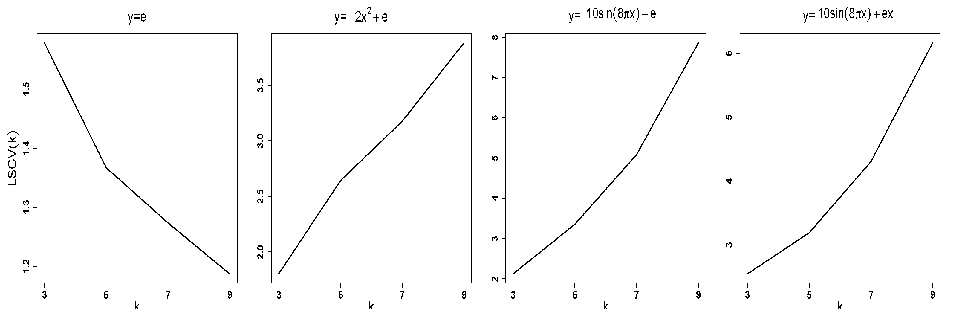
In the continuous case with k-nearest neighbor estimation, the average of a big proportion of Y values is used to approximate the response variable if a large k value is utilized. As a consequence, bigger k tends to give larger least squares error when the regression function is under the alternative hypothesis. This is especially true when the regression function has substantial curvature, such as in high frequency alternatives. On the other hand, larger k tends to give smaller least squares error when the data were generated under the constant regression null hypothesis.

In either case, the smallest value for k is 3 (note: $k=1$ corresponds to the case of no data augmentation). In order to keep the least squares error minimized under the alternative hypothesis and reasonable under the null hypothesis, we recommend to let $\kappa$ contain a few small integer values. For example, $\kappa =\{3,5\}$, which is a safe choice for both moderate and large sample sizes.

Figure 1 shows the typical pattern of $LSCV\left(k\right)$ as a function of k for $k=3,5,7,9$ when the response variable was generated as (1) $Y_i=e_i$; (2) $Y_i=2X_i^2+e_i$; (3) $Y_i=10sin\left(8\pi X_i\right)+e_i$; and (4) $Y_i=10sin\left(8\pi X_i\right)+e_i{X}_i$, where $e_i$ and $X_i$ are i.i.d $\sim N(0,1)$.

3. Monte Carlo Simulation Studies

In this section, we present the results of some simulation studies to investigate the type I error and power performance of our test. The test has a parameter k to specify the number of nearest neighbors for data augmentation. The inference for our test requires the k to be a small odd positive integer. We report the results for $k=3$ and 5 and denote them as $G_{N3}$ and $G_{N5}$, respectively. This is for the user to have an idea of how the test behaves with a given k. Furthermore, we report the results of our test with k selected from 3 and 5 using our considered method in Section 2.4 and denote it as $G_N$. For the $G_N$ applied to each generated data set, the value of the k is selected using $\widehat{k}$ in (20), and our test with parameter $\widehat{k}$ is used to obtain the p-value.

For comparison, we also report the corresponding results for the test of Reference [16], the order selection (OS) test of Reference [1], the rank-based test (ROS) of Reference [2], the bootstrap order selection test (BOS) of Reference [5], and the Bayes sum test of Reference [3]. As argued in Section 7.1 of Reference [4], evenly spaced design points should be used for calculation of these four test statistics even when they are unevenly spaced. So, the generated covariate values in increasing order were replaced by evenly spaced design points on $(0,1)$ for all four tests. For BOS, we apply the wild bootstrap algorithm of Reference [5] based on the residuals $Y_i-\overline{Y},i=1,\dots ,n,$ and use their test statistic with 1000 bootstrap samples for each replication. For the Bayes sum test, we use the statistic that has been reported to have good power from a comprehensive simulation study in Reference [3]. For approximating the p-values of the Bayes sum test, Hart [3] gave two versions of the approximation, one assuming normality (BN) and one using the bootstrap (BB). For BN, a random sample of the same sample size as the data was generated from the standard normal distribution, and the Bayes sum test statistic was calculated from the data so generated, regardless of the actual distribution of the response variable. The process was independently repeated 10,000 times, and the p-value was obtained based on the empirical distribution of these 10,000 values. For BB, the bootstrap samples were drawn from the empirical distribution of the residuals $Y_i-\overline{Y}$, $i=1,\dots ,n$, rather than the normal distribution, and the p-value approximation was carried out similarly. The scale parameter ${\sigma }^2$ for a given data set $Y_1,\dots ,Y_n$ in both BB and BN statistics was estimated by ${\widehat{\sigma }}^2={(n-2)}^{-1}{\sum }_{i=2}^{n-1}{(0.809Y_{i-1}-0.5Y_i-0.309Y_{i+1})}^2$, as was suggested in Reference [3]. It was reported in Reference [3] that the results obtained using the normality assumption were in basic agreement with those obtained using the bootstrap. So, we only report the simulation results for BN.

The values for the covariate X were independently generated from Uniform$(0,1)$. First, we consider the performance of different tests under the $H_0$. The data were generated from

$$\begin{array}{c}\hfill \mathrm{Model} M_0:Y_i=10+{ϵ}_i,\end{array}$$

where the error term ${ϵ}_i$ were independently generated with one of the four error distributions:

1.

${ϵ}_i\sim$ Uniform$(-0.1,0.1)$ (denoted as Unif in

Table 1. Percent of rejection at 0.05 level under $H_0$ for data generated from Model $M_0$. OS: order selection test of Reference [1]; BN: Reference [3] Bayes sum test with Normal approximation; BOS: order selection test with wild bootstrap of Reference [5]; ROS: rank-based test of Reference [2]; WAI3, WAI5, WAI7: test of Reference [16] with $k=3$, 5, and 7, respectively; $G_N$: the proposed test with $k=3$, 5, 7, and $\widehat{k}$ from (20). Highly inflated empirical type I errors are marked with red color.

	${\mathit{ϵ}}_{\mathit{i}}\sim$Normal and$\mathit{n}=$					${\mathit{ϵ}}_{\mathit{i}}\sim$Unif and$\mathit{n}=$
Test	25	50	75	100	200	25	50	75	100	200
BN	4.25	4.90	5.40	5.70	4.45	5.20	6.15	5.45	4.85	4.95
OS	4.35	5.55	5.05	5.50	3.65	4.70	5.60	5.00	4.95	5.10
ROS	3.50	4.95	4.95	5.55	3.70	3.95	5.90	5.20	4.60	5.10
BOS	3.85	5.45	5.05	5.85	4.00	4.35	5.65	6.00	5.15	5.15
WAI   $k_n=3$	8.75	7.25	7.10	7.35	6.40	8.90	9.05	8.20	7.55	6.65
WAI   $k_n=5$	6.85	5.85	6.25	6.40	6.15	6.85	8.40	7.05	6.80	6.45
WAI   $k_n=7$	5.00	5.20	5.40	6.25	6.30	5.75	8.10	6.30	6.35	6.40
$G_N$    $k=3$	5.60	4.05	4.10	3.95	3.45	5.40	4.95	4.30	3.30	3.05
$G_N$    $k=5$	4.40	3.45	3.80	3.90	3.35	4.45	5.15	3.95	3.80	3.80
$G_N$    $k=7$	3.65	3.45	4.15	4.40	4.00	3.60	5.20	4.25	3.95	4.25
$G_N$    $\widehat{k}$	6.20	5.95	4.95	4.65	4.60	6.00	4.85	4.85	5.15	4.35
	${ϵ}_{\mathit{i}}\sim \mathit{T}\left(\mathbf{5}\right)/\mathbf{30}$and$\mathit{n}=$					${ϵ}_{\mathit{i}}\sim$Heter and$\mathit{n}=$
Test	25	50	75	100	200	25	50	75	100	200
BN	4.15	4.95	4.75	4.70	5.15	8.95	9.20	7.95	8.55	7.05
OS	3.70	4.35	5.20	4.20	4.65	6.40	7.65	7.85	7.95	7.20
ROS	4.40	4.45	4.85	4.50	5.10	5.70	7.00	7.55	7.25	7.10
BOS	3.75	4.90	5.25	4.45	5.20	4.70	5.45	5.10	5.45	4.95
WAI   $k_n=3$	8.75	8.85	8.40	7.20	6.95	12.50	10.05	11.50	10.20	8.10
WAI   $k_n=5$	6.50	7.25	6.85	6.10	5.90	9.05	9.10	9.55	9.15	7.50
WAI   $k_n=7$	4.65	6.30	5.60	5.35	6.00	6.80	7.80	7.50	8.45	7.95
$G_N$    $k=3$	3.80	3.45	2.50	1.95	1.95	7.50	5.80	6.45	6.50	5.00
$G_N$    $k=5$	3.10	3.25	2.65	1.70	1.80	5.30	5.65	6.30	6.15	4.40
$G_N$    $k=7$	2.50	2.95	2.80	2.25	1.95	4.85	5.40	5.30	6.10	5.20
$G_N$    $\widehat{k}$	4.30	3.95	3.60	2.55	2.05	8.20	6.70	7.40	6.90	5.00

and

Table 2. Percent of rejection under high frequency alternatives $M_1$ to $M_4$ with $q=8$ and sample size $n=50$. The legend of the tests are same as in Table 1. WAI is not included since it could not keep its type I error under control. Note: BN also has highly elevated type I error in the Heteroscedastic case.

	${\mathit{ϵ}}_{\mathit{i}}\sim$Normal					${\mathit{ϵ}}_{\mathit{i}}\sim$Unif
Model	BN	OS	ROS	BOS	${\mathit{G}}_{\mathit{N}}$	BN	OS	ROS	BOS	${\mathit{G}}_{\mathit{N}}$
$M_1$	100	78.35	71.65	66.70	100	100	78.35	72.20	66.85	100
$M_2$	100	87.75	80.70	91.55	100	100	87.70	81.00	91.95	100
$M_3$	99.65	70.70	70.25	43.15	99.70	99.50	67.85	63.00	41.15	99.60
$M_4$	99.05	61.75	52.20	34.45	99.60	81.15	17.35	11.60	10.25	93.20
	${ϵ}_{\mathit{i}}\sim \mathit{T}\left(\mathbf{5}\right)/\mathbf{30}$					${ϵ}_{\mathit{i}}\sim$Heter
Model	BN	OS	ROS	BOS	${\mathit{G}}_{\mathit{N}}$	BN	OS	ROS	BOS	${\mathit{G}}_{\mathit{N}}$
$M_1$	100	78.35	71.70	67.30	100	100	78.40	72.25	66.45	100
$M_2$	100	87.50	80.55	92.00	100	100	87.75	80.75	91.95	100
$M_3$	99.60	69.20	66.95	42.40	99.65	99.60	69.85	67.65	43.40	99.65
$M_4$	92.30	29.80	21.20	15.90	97.35	97.05	44.75	32.20	23.45	99.40

);

2.

(Normal) ${ϵ}_i\sim$ Normal$(0,0.{02}^2)$ (denoted as Normal in Table 1 and Table 2);

3.

${ϵ}_i=V_i/30$, where $V_i$ follows t-distribution with 5 degrees of freedom (denoted as $T\left(5\right)/30$ in Table 1 and Table 2); and

4.

${ϵ}_i=X_i·e_i$, where $e_i\sim$ Uniform$(-0.1,0.1)$. This is a heteroscedastic regression model and denoted as Heter in Table 1 and Table 2.

The empirical type I error rates (in percentage) under $H_0$ are reported in Table 1. It can be seen that the test of Reference [16] with $k_n=3$ or 5 generally has inflated type I error and is particularly serious with smaller sample sizes. For $k_n=7$, their test has type I error close to 0.05 when the error distribution is Normal or T(5)/30 but is as high as about twice of the significance level in the heteroscedastic case. Its performance for $k_n=7$ is better than with other $k_n$ values but still is inflated for the heteroscedastic case. The order selection test of Reference [1] and the proposed test with different k-values have better type I error control. Among the three k-values, larger k pulls more observations around each covariate value as pseudo replicates. This could lead to the test being less sensitive to curvature departure against the null hypothesis. Hence, we recommend to choose k between 3 and 5.

Next, we consider the performance of the tests with data generated from nonlinear models. The response values were independently generated according to the following four models for $i=1,\dots ,n$, with the moderate sample size of $n=50$ in all cases:

• Model $M_1$: $Y_i=10cos\left(q\pi X_i\right)+{ϵ}_i$,
• Model $M_2$: $Y_i=10sin\left(q\pi X_i\right)+{ϵ}_i$,
• Model $M_3$: $Y_i=e^{-2X_i}cos\left(q\pi X_i\right)+{ϵ}_i$, and
• Model $M_4$: $Y_i=0.2e^{-2X_i}cos\left(q\pi X_i\right)+{ϵ}_i$,

where q in Models $M_1$–$M_4$ represents the frequency. We considered $q=8$ and $q=2$. The case with $q=8$ is a higher frequency alternative compared to those reported in Reference [3]. The data for the error term ${ϵ}_i$ in each model were independently generated with one of the four error distributions listed earlier. Model $M_0$ serves as the null model to obtain the type I error rates for all tests. For each error distribution, the data were generated from Models $M_0$–$M_4$, with sample size $n=50$ for 2000 times, and the rejection rates (in percentage) at significance level 0.05 are reported in Table 2.

It can be seen that the type I error estimates for all tests were below or close to the nominal level 0.05 for all models with homoscedastic errors. For the heteroscedastic regression model, the variance of the error depends on the covariate, while the conditional mean of the response variable given the covariate is a constant under Model $M_0$. In this case, all the tests tend to be liberal.

The rows $M_1$ to $M_4$ in Table 2 show the power comparison for the different combinations between Models $M_1$–$M_4$ and the four types of the error distribution. The powers of our test with $\widehat{k}$ ($G_N$) are higher than all other tests in all cases. BN has power close to our test. OS, ROS, and BOS fall far behind. The low power performance of BOS in the case of high frequency alternatives was mentioned in Reference [5], and they suggested (without details) to use smoothing squared residuals to deal with that.

It is noticeable that the power of our test is 1 for Models $M_1$ and $M_2$ for all different types of the error distribution and very close to 1 for Models $M_3$ and $M_4$. In addition, the power for OS was slightly higher than that for ROS in all cases.

Models $M_3$ and $M_4$ are similar, except that Model $M_4$ has lower signal to noise ratio than Model $M_3$. With the lower signal to noise ratio, the power for ROS, OS and BOS drops drastically. To have a closer look at the numerical performance of all tests under local alternatives, we considered the model $Y_i=C{e}^{-2X_i}cos\left(8\pi X_i\right)+{ϵ}_i$, with $C=0.1,0.12,0.14,0.16,0.18$ and ${ϵ}_i\sim$ Uniform$(-0.1,0.1)$. The empirical power curves are given in Figure 2. It is obvious that our test $G_N$ has consistently higher power than the other tests.

The discussions above are for high frequency alternatives with $q=8$ and moderate sample size $n=50$. When sample size increases, while the frequency stays the same, the power of each test also increases. For sample size of 100, the empirical power is 1 for all the compared tests of NB, OS, ROS, and $G_N$ under Models $M_1$–$M_3$. Under Model $M_4$, OS and ROS have power slightly below 1 for the case with uniform error. The rest of the tests have power close to 1. Similarly, for lower frequency alternatives, for example, when $q=2$ and $n=50$, all these tests have power close to 1.

To examine how the power of these tests changes with the sample size, we generated data with model $Y_i=N^{-1/4}A\left(X_i\right)+{ϵ}_i$, where $A\left(X_i\right)=0.3e^{-2X_i}cos\left(8\pi X_i\right)$, ${ϵ}_i\sim$ Uniform$(-0.1,0.1)$, for $N=15,25,50,75,100,125,150,175,200,250$. The empirical power of these tests is presented in Figure 3, where $G_N$ is our test with $\widehat{k}$ selected from $k=3$ and 5 based on (20). It is obvious that the proposed test $G_N$ consistently has the highest power over all the sample sizes considered.

Even though BN showed a comparable performance to our test $G_N$ in many cases, the running time of BN is much longer than $G_N$. In particular, the average running time from 10,000 runs from BEOCAT cluster machines for $G_N$ is 0.03 s, while that for BN is 9.7 s. So, $G_N$ is more than 300 times faster than BN.

4. Applications to Real Data

4.1. Application to Gene Expression Data from Patients Undergoing Radical Prostatectomy

In this subsection, we present an application of our test to gene expression data from patients undergoing radical prostatectomy in order to predict the behavior of Prostate cancer. This data set was collected between 1995 and 1997 at the Brigham and Women’s Hospital from 52 tumor and 50 normal prostate samples using oligonucleotide microarrays containing probes for 12,600 genes and expressed sequence tags (the data is available at https://www.ncbi.nlm.nih.gov/gds/?linkname=pubmed_gds&from_uid=12086878 on 11 July 2021). The data shows heterogeneity and has a binary response variable which is the patient outcome (tumor or normal). Applying our test to the expression data from each gene, we identified 980 genes that are significantly associated with the response variable after Bonferroni correction $(p\le 0.001/$12,600). On the other hand, Singh et al. [23] used permutation test to identify important genes. They found 456 genes whose expression values are significantly correlated with patient outcome $(p\le 0.001)$. Note that the significance declared by Reference [23] is at 0.001 level without any multiple comparison adjustment. Ours are obtained at the same significance level but with the Bonferroni control, which is a very conservative method for multiple comparison adjustment. With such conservative control, we still identified more than twice of the genes than Reference [23]. It is worth mentioning that our test was developed under very general assumptions that are expected to hold true for the microarry data here. These results suggest that our test is much more powerful than the permutation test of Reference [23]. Furthermore, we performed k-nearest neighbor (KNN) classification on the data for the top i genes (i genes with smallest p-values, $i=1,2,\cdots ,980$) to predict the patient outcomes. The leave-one-out cross validation (LOOCV) was used as a validation method. The parameter k in KNN was estimated with the training part of the data in LOOCV procedure by the profile pseudolikelihood method of Reference [22]. The leave-one-out accuracy curve with increasing number of selected top i genes is shown in Figure 4. We would like to comment that these genes were obtained individually. Our simple application of the test is not meant to find the best combination of genes that have the best classification accuracy. Even under such circumstances, the top genes found with our test give good LOOCV accuracy.

4.2. Application to Assess Richards Growth Curve Fit for the COVID Cases and Deaths

In this application, we would like to assess if the popular Richards growth model can fit the COVID-19 cases or deaths for the U.S.

The Richards growth curve model has been adapted recently for real-time prediction of outbreak of diseases in epidemiology. Below is a form of the the Richards curve $f(t;{\theta }_1,{\theta }_2,{\theta }_3,\xi )$ that was used to fit the COVID-19 outbreak in Reference [24]:

$$\begin{array}{c}\hfill f\left(t;{\theta }_1,{\theta }_2,{\theta }_3,\xi \right)={\theta }_1·{\left[1+\xi ·exp\left\{-{\theta }_2·\left(t-{\theta }_3\right)\right\}\right]}^{-1/\xi },\end{array}$$

where ${\theta }_1$, ${\theta }_2$, and ${\theta }_3$ are real numbers, and $\xi$ is a positive real number.

Using this parameterization of the Richards curve, Lee et al. [24] stated that, given a progression constant $\gamma$ with $0<\gamma <1$, the flat time point $t_{flat,\gamma }$ is given by

$$\begin{array}{c}\hfill t_{flat,\gamma }={\theta }_3-\frac{1}{{\theta }_2}·log\left[\frac{1}{\xi }·\left\{{\left(\frac{1}{\gamma }\right)}^{\xi }-1\right\}\right],0<\gamma <1.\end{array}$$

They predicted that the posterior means of the flat time points $t_{flat,\gamma }$ for the U.S. to be 30 May, 16 July, 30 August, and 15 October when the corresponding $\gamma$’s are chosen by 0.9, 0.99, 0.999, and 0.9999, respectively. However, as of the end of 2020, the COVID-19 confirmed cases are still continuing to climb up. This is an evidence that the Richards curve does not fit the COVID-19 infection growth well.

We downloaded the cumulative number of confirmed cases of U.S. COVID-19 historical data from https://covidtracking.com/data/download/national-history.csv on 12 July 2021. This website stopped tracking COVID in late March 2021. We also downloaded the daily number of death counts for U.S. COVID-19 data from the CSSE data repository of Johns Hopkins University at https://github.com/CSSEGISandData/COVID-19 on the same day. The data contains death counts up to 11 July 2021.

To fit a Richards curve for each data set, we only included data on days such that the cumulative count is at least seven and removed the last ten days’ data so that those ten days’ counts could be used as an additional out-of-sample assessment of the model fit. A separate Richards curve was fitted for the daily cumulative confirmed cases and deaths. Figure 5 shows the nonlinear least squares fitted Richards growth curves and the observed counts. The fitted curve also contains prediction for the future 10 days beyond the observed days.

Table 3. Parameters of the Richard growth models, $R^2$ between the observed and model estimated counts, and the p-values of the lack of fit test.

	${\mathit{\theta }}_1$	${\mathit{\theta }}_2$	${\mathit{\theta }}_3$	$\mathit{\xi }$	${\mathit{R}}^2$	p-Value of ${\mathit{G}}_{\mathit{N}}$
U.S. deaths	594,331	0.0452	−17.1062	6.8505	0.9950	0.0000
U.S. confirmed cases	27,890,138	0.1270	−43.7943	11.5151	0.9982	0.0000

gives the correlation coefficients between the observed counts and the estimated count. Even though the $R^2$s between the fitted curves and observed numbers are over 99%, the p-values for the lack-of-fit tests are both essentially 0. The Richards curve seems to be better at predicting the number of confirmed cases than predicting the number of deaths. It appears that the pandemic progression is more complicated than the Richards curve due to changes in social distancing, stay-at-home order policies, and vaccine availability. U.S. holidays, such as Thanksgiving and Christmas, also contributed drastically to the increase of count in late November. The ${\theta }_1$ parameter predicts the epidemic size. For the total number of deaths, the model predicted epidemic size is 594,331. For the confirmed cases, the model predicted size is around 27.9 million. Both numbers underestimate the true epidemic size. As of 12 July 2021, the U.S. confirmed cases is over 33.8 million, and the number of U.S. deaths is 606,000. These numbers are much larger than the model predicted size, suggesting that the Richards curves could not model the confirmed cases or deaths adequately.

5. Conclusions

In this paper, we derived the asymptotic distribution of a nonparametric lack-of-fit test of constant regression in the presence of heteroscedastic variances. We considered a test statistic obtained using the augmentation of a small number of k-nearest neighbors defined through the ranks of the predictor variable. The test statistic is the studentized version of the difference of two quadratic forms. Both of two quadratic forms estimate a common quantity under the null hypothesis but they converge to different quantities under any alternatives The asymptotic distribution of the difference was also given in Reference [16] but with a biased asymptotic variance. We derived the correct form of the asymptotic distribution of the test statistic under both the null hypothesis and local alternatives. In addition, we also provided a procedure to choose the parameter k based on the Least Squares Cross-Validation idea used in k-nearest neighbor regression. Our test has several advantages. It provides a unified framework for testing lack-of-fit for a given regression function when the response is either a discrete or a continuous random variable and the covariate is a continuous variable. This makes it convenient for unified inferences and applications. There is no need to assume the distribution of the data, which makes the test widely applicable to many practical data. The fixed number of nearest neighbors augmentation ensures good power to detect both low and high frequency alternatives even for moderate sample sizes, and the parametric standardizing rate for the test statistic is achieved. The test statistic is easy and fast to calculate. Our simulation studies show that the test is more powerful than some well known competing test procedures when data are generated under high frequency alternatives. Therefore, the results in this paper offer a useful tool for lack-of-fit testing.

References

1. Eubank, R.L.; Hart, J.D. Testing goodness-of-fit in regression via order selection criteria. Ann. Statist. 1992, 20, 1412–1425. [Google Scholar] [CrossRef]
2. Hart, J. Smoothing-inspired lack-of-fit tests based on ranks. In Beyond Parametrics in Interdisciplinary Research: Festschrift in Honor of Professor Pranab K. Sen; Institute of Mathematical Statistics: Beachwood, OH, USA, 2008; Volume 1, pp. 138–155. [Google Scholar]
3. Hart, J. Frequentist-Bayes lack-of-fit tests based on Laplace approximations. J. Stat. Theory Pract. 2009, 3, 681–704. [Google Scholar] [CrossRef]
4. Hart, J. Nonparametric Smoothing and Lack-of-Fit Test; Springer: New York, NY, USA, 1997. [Google Scholar]
5. Chen, C.-F.; Hart, J.D.; Wang, S. Bootstrapping the order selection test. J. Nonparametr. Stat. 2001, 13, 851–882. [Google Scholar] [CrossRef]
6. Kuchibhatla, M.; Hart, J.D. Smoothing-based lack-of-fit tests: Variations on a theme. J. Nonparametr. Stat. 1996, 7, 1–22. [Google Scholar] [CrossRef]
7. Lee, B.J. A Nonparametric Model Specification Test Using a Kernel Regression Method. Ph.D. Thesis, University of Wisconsin, Madison, WL, USA, 1988. [Google Scholar]
8. Yatchew, A.J. Nonparametric regression tests based on least square. Econom. Theory 1992, 8, 435–451. [Google Scholar] [CrossRef]
9. Eubank, R.L.; Spiegelman, C.H. Testing the goodness of fit of a linear model via nonparametric regression techniques. J. Am. Stat. Assoc. 1990, 85, 387–392. [Google Scholar] [CrossRef]
10. Hardle, W.; Mammen, E. Comparing nonparametric versus parametric regression fits. Ann. Statist. 1993, 21, 1926–1947. [Google Scholar] [CrossRef]
11. Zheng, J.X. A consistent test of functional form via nonparametric estimation techniques. J. Econom. 1996, 75, 263–289. [Google Scholar] [CrossRef]
12. Horowitz, J.Z.; Spokoiny, V.G. An adaptive, rate-optimal test of a parametric mean-regression model against a nonparametric alternative. Econometrica 2001, 69, 599–631. [Google Scholar] [CrossRef]
13. Guerre, E.; Lavergne, P. Data-driven rate-optimal specification testing in regression models. Ann. Statist. 2005, 33, 840–870. [Google Scholar] [CrossRef] [Green Version]
14. Song, W.; Du, J. A note on testing the regression functions via nonparametric smoothing. Can. J. Stat. 2011, 39, 108–125. [Google Scholar] [CrossRef]
15. Wang, L.; Akritas, M. Testing for covariate effects in the fully nonparametric analysis of covariance model. J. Am. Stat. Assoc. 2006, 101, 722–736. [Google Scholar] [CrossRef]
16. Wang, L.; Akritas, M.G.; Van Keilegom, I. An ANOVA-type nonparametric diagnostic test for heteroscedastic regression models. J. Nonparametr. Stat. 2008, 20, 365–382. [Google Scholar] [CrossRef]
17. Wang, H.; Tolos, S.; Wang, S. A distribution free test to detect general dependence between a response variable and a covariate in the presence of heteroscedastic treatment effects. Can. J. Stat. 2010, 38, 408–433. [Google Scholar] [CrossRef]
18. Hardle, W.; Hall, P.; Marron, J.S. How far are automatically chosen regression smoothing parameters from their optimum? J. Am. Stat. Assoc. 1988, 83, 86–95. [Google Scholar]
19. Wang, H.; Akritas, M. Asymptotically distribution free tests in heteroscedastic unbalanced high dimensional anova. Stat. Sin. 2011, 21, 1341–1377. [Google Scholar] [CrossRef] [Green Version]
20. de Jong, P. A central limit theorem for generalized quadratic forms. Probab. Theory Relat. Fields 1987, 75, 261–277. [Google Scholar] [CrossRef]
21. Hart, J.D.; Yi, S. One-sided cross-validation. J. Am. Stat. Assoc. 1998, 93, 620–631. [Google Scholar] [CrossRef]
22. Holmes, C.C.; Adams, N.M. Likelihood inference in nearest-neighbour classification models. Biometrika 2003, 90, 99–112. [Google Scholar] [CrossRef] [Green Version]
23. Singh, D.; Febbo, P.G.; Ross, K.; Jackson, D.G.; Manola, J.; Ladd, C.; Tamayo, P.; Renshaw, A.A.; D’Amico, A.V.; Richie, J.P.; et al. Gene expression correlates of clinical prostate cancer behavior. Cancer Cell 2002, 1, 203–209. [Google Scholar] [CrossRef] [Green Version]
24. Lee, S.Y.; Lei, B.; Mallick, B.; Samy, A.M. Estimation of covid-19 spread curves integrating global data and borrowing information. PLoS ONE 2020, 15, e0236860. [Google Scholar] [CrossRef] [PubMed]
25. Pyke, R. Spacings (with discusssion). J. R. Stat. Soc. Ser. B Stat. Methodol. 1965, 27, 395–449. [Google Scholar]
26. Bishop, Y.M.; Fienberg, S.E.; Holland, P.W. Discrete Multivariate Analysis; Springer: New York, NY, USA, 2007. [Google Scholar]
Figure 1. Typical patterns of L S C V ( k ) versus k in continuous data.
Symmetry 13 01264 g001
Figure 2. Empirical power of the tests for data generated from Y i = C e 2 X i c o s ( 8 π X i ) + ϵ i with sample size n = 50 and ϵ i Uniform ( 0.1 , 0.1 ) . Due to small values of C, the signal to noise ratio is low. WAI is not included since it could not keep its type I error under control for this sample size and the uniform error distribution.
Symmetry 13 01264 g002
Figure 3. Empirical power for different sample sizes. The data were generated from Y i = N 1 / 4 0.3 e 2 X i c o s ( 8 π X i ) + ϵ i , where ϵ i Uniform ( 0.1 , 0.1 ) . As the sample sizes N increases, the power of all tests increases. The G N test approaches 1 much faster than other tests. WAI is not included since it could not keep its type I error under control for the sample sizes and the uniform error distribution.
Symmetry 13 01264 g003
Figure 4. The leave-one-out accuracy curve with increasing number of selected genes.
Symmetry 13 01264 g004
Figure 5. Observed U.S. COVID-19 mortality and confirmed cases with the Richards growth curve estimates.
Symmetry 13 01264 g005