Abstract
A natural example of evolution can be described by a time-dependent two degrees-of-freedom Hamiltonian. We choose the case where initially the Hamiltonian derives from a general cubic potential, the linearised system has frequencies 1 and . The time-dependence produces slow evolution to discrete (mirror) symmetry in one of the degrees-of-freedom. This changes the dynamics drastically depending on the frequency ratio and the timescale of evolution. We analyse the cases where the ratio’s 1,2 turn out to be the most interesting. In an initial phase we find 2 adiabatic invariants with changes near the end of evolution. A remarkable feature is the vanishing and emergence of normal modes, stability changes and strong changes of the velocity distribution in phase-space. The problem is inspired by the dynamics of axisymmetric, rotating galaxies that evolve slowly to mirror symmetry with respect to the galactic plane, the model formulation is quite general.
MSC:
34C14; 34C29; 34E10; 37J25; 37J65; 70H11; 85A05
1. Introduction
There are many non-autonomous dynamical systems with evolutionary aspects but the necessary theory for understanding them is still restricted to linear systems with equations that have a limit as time increases (see [1] Chapter 3). The main reason for this is probably that understanding steady state, autonomous, nonlinear systems is already a formidable task. Physical examples where explicit time-dependence plays a part are the evolution to spherical structures in nature and on solar system scale planetary satellite systems evolving by long-term tidal forces to more symmetric orbits (for references see [2]). Explicit time-dependence also is ubiquitous in engineering systems but there it is usually concerned with short-time transient phenomena or time-periodic influences.
We will consider Hamiltonian systems where explicit time-dependence slowly vanishes producing the transition from a system that is asymmetric in some sense to a Hamiltonian system with symmetry. In [3] a 1-dimensional cartoon problem is considered where time-dependent asymmetric terms vanish with time; it is of the form:
A dot means differentiation with respect to time, 2 dots second order differentiation with respect to time, is a positive small pameter. The function is monotonically decreasing from the value 1 to zero. Equation (1) models slow evolution to symmetric dynamics in the sense that the asymmetric potential vanishes with time; although the equation is simple it shows already a relation with dissipative systems and the construction of a global adiabatic invariant.
In [2] a 2 degrees-of-freedom (dof) system is considered with a cubic potential that is discrete symmetric in one of the positions () and asymmetric in the other position (). The Hamiltonian is:
As before the asymmetric term vanishes slowly, the system evolves to a 2 -dimensional harmonic oscillator. Again a relation with dissipative systems can be established, 2 adiabatic invariants can be found. The system displays overall dynamics that keeps some information from its asymmetric past.
In the sequel we will study evolution in two dof Hamiltonian systems keeping nonlinearities. That makes the models both more realistic and more complicated.
In this paper we describe an evolutionary system (14) inspired by the evolution of a rotating galaxy. It is important to note that this system in its general formulation of a time-dependent Hamiltonian system extends to many other physical problems apart from those derived from this particular application.
Set-Up of the Paper
In Section 2 we describe the dynamics of rotating stellar systems and we formulate the equations for the axisymmetric case. These formulations have been known a long time in astrophysics but we summarise this for a more general audience. In the sequel we describe the dynamics of prominent resonances producing periodic solutions, adiabatic invariants and stability changes during evolution.
In Section 3 we formulate the time-dependent Hamiltonian where the terms that are not discrete (mirror) symmetric with respect to the galactic plane are slowly vanishing with time. This leads to the slow-fast system (14) where the fast motion is described by a family of discrete symmetric two dof freedom Hamiltonian systems with resonances.
Section 4 describes the reformulation of system (14) suitable for averaging-normalisation while using a modification of averaging developed in an appendix (Section 9). It is shown that the system for evolution to symmetry is equivalent with a dissipative system.
The prominent resonance 1:2 is studied in Section 5. The results are surprising as first order averaging-normalisation producing approximations valid on an interval of size yields no epicyclic normal mode and an unstable vertical normal mode. Second order averaging-normalisation producing approximations valid on an interval of size show that after a long time the epicyclic and vertical normal modes arise and are stable. These changes of presence and stability have drastic consequences for the evolution of the overall dynamics of the system.
In contrast to the preceding case, the 1:3 resonance is dynamically less interesting (Section 6). We have in this case basically the dynamics of the 2:6 resonance that is described by higher order resonance techniques from [4].
In Section 7 the dynamics of the 1:1 resonance turns out to be the most complicated case. Second order averaging-normalisation is necessary to describe the dynamics. Depending on the system parameters we find again normal modes and stability changes during evolution. Explicit examples include the evolution to the Hénon-Heiles potential.
After the concluding discussion we present in Section 9 a brief survey of the averaging theorems we have used in this paper. For the proofs we indicate the relevant literature.
Numerics. For the computation of the figures we have used Matcont (free access) under MatLab (licensed). The algorithm used is ode 78 with relative and absolute errors exp.(−15).
2. The Dynamics of the Milky Way
In this section we will summarise the formulation for rotating stellar systems and we will specialise this to the axisymmetric case. The modelling was used in [5] and can also be found in [6].
2.1. The Collisionless Boltzmann Equation
The reasonable looking approximation of few collisions in stellar systems raises questions on the statistical mechanics of these systems. Another basic assumption often made in model building for galaxies is most of the systems being in equilibrium. A more realistic assumption is quasi-static equilibrium that leaves room for evolution to this stage. In this paper the choice of a time-dependent Hamiltonian will be the basis for studying such models of evolution and the quite remarkable consequences.
The collisionless Boltzmann or Liouville equation describes the distribution of n particles, stars in this case, in dimensional phase-space. One has to add the Poisson equation for self-gravitation. A good description with examples can be found in [6] Chapter 4. The equation for the distribution of particles where indicates the position, the velocity, is the continuity or Liouville equation in dimensional phase-space with clearly the assumption that no particle escapes, is destroyed or is created in the system. With Lagrangian derivative the Liouville equation is . If the collective gravitational potential ruling the dynamics of the system is , the Liouville equation becomes explicitly:
The characteristics of this first order partial differential equation are given by the Hamiltonian equations of motion. The solutions of the Hamiltonian system produce according to Monge the solutions of the Liouville equation as they represent the geometric sets where the solutions of the Liouville equation are constant. This procedure is very effective if we find not only solutions but integrals of motion that contain sets of solutions. Assuming for instance a time-independent potential and axi-symmetry, we have already 2 independent integrals of motion, energy E and angular momentum L with respect to the axis of rotation. Any differential function f of E and L will satisfy the Liouville equation. It was noted very early that such solutions will produce velocity distributions that are symmetric perpendicular to and in the direction of the rotation axis. This does not agree with observations in our own galaxy, in fact the two dispersions differ considerably; for velocity dispersions in the plane of the galaxy see [7], for dispersions in the halo [8]. Velocity dispersions in galaxies is an ongoing research topic, the reader interested in recent observational results might google the authors Rachel Bezanson, M. Franx and P.G. van Dokkum.
The velocity asymmetry triggered off a long search for “a third integral of the galaxy” that came to an important point in the 1960’s when it was shown in Arnold-Moser theory that such 3rd integrals in general do not exist but that an infinite number of so-called KAM-tori corresponding with approximate first integrals may survive. This near-integrability caused a lot of confusion in the literature.
One of the aims of our study is to investigate whether evolution from an asymmetric state to a near-integrable symmetric dynamical state might influence the velocity distributions as if the system “remembers” its asymmetric past.
From [6] Chapter 4 we consider the dynamics in cylindrical coordinates with ; we have with potential the equations of motion:
Solving system (4) and obtaining (approximate) first integrals enables us to describe families of distribution functions that satisfy the Liouville Equation (3).
In the sequel we assume that the systems to be considered have reached the axi-symmetric state. Initially the systems are not mirror-symmetric with respect to a plane, they evolve slowly in time to such a state.
2.2. Rotating Axi-Symmetric Models
We will consider models that are inspired by axisymmetric rotating galaxies. One can think of disk galaxies or rotating flattened elliptical galaxies. The axisymmetry expressed by
produces the angular momentum integral J (in [6] called ) enabling us to reduce spatial 3-dimensional motion to 2 degrees of freedom (dof). We have with Equations (4) and (5)
leading to the angular momentum integral
The equations of motion (4) can be written as
In the equatorial plane that is perpendicular to the axis of rotation we have circular orbits at where the rotation speed matches constant angular momentum:
We will expand the Hamilitonian around the circular orbits. In most models, the potential is assumed to be mirror (discrete) symmetric with respect to the equatorial plane. In cylindrical coordinates with z in the direction of the rotation axis and corresponding with the equatorial plane we will put in a final stage of evolution . The evolution towards this symmetric state is caused by mechanisms unknown to us, maybe contraction combined with rotation or dynamical friction plays a part. We propose to avoid the speculative description of complicated mechanisms by introducing a function of time slowly destroying the asymmetric potential.
Around the circular orbits in the galactic plane we find epyciclic orbits in the R-direction nonlinearly coupled to bounded vertical motion in the z-direction. An early study of such orbits in a steady state galaxy model is [5], for a systematic evaluation of the theory see [6]. A detailed analysis of the orbits can be found in [9]. A simplifying transformation from [5] is to use the reduced potential
leading to the equations of motion:
3. Shortcut to a Model with Evolution
We want to describe the dynamical consequences of evolution to an axi-symmetric state by expanding around the circular orbits at position putting . To study evolution to symmetry we consider as a model the time-dependent two dof Hamiltonian:
The epicyclic frequency in the galactic plane has been scaled to 1, the vertical frequency is , so x corresponds with deviations of . The function is continuous and monotonically decreasing from to zero; we will usually choose with . If we have the famous Hénon-Heiles problem [10].
A detailed modelling of the evolution of a large contracting cloud to an axisymmetric galaxy is not available. The model presented here ignores all special types of dynamics as for instance the formation of new stars, dissipation by gas cloud motions or the spectacular emergence of high-velocity stars by supernovae in binary stars.
The evolution to a time-independent Hamiltonian is also clear when considering the Lagrangian derivative:
The energy given by (10) decreases slowly. Near the circular orbits, the time-dependent perturbation factor decreases monotonically, the change of the energy will be small and depends on the signs of and the behaviour of . On the other hand the quantitative dynamical consequences of the asymmetric potential in the transitional stage can be considerable and depends on the size of and .
The quadratic part is called , the cubic part . The coefficients are free parameters with , represents the frequency ratio of the 2-dof oscillators with prominent resonances . The possible values of depend on the galactic potential constructed. An example describing an axisymmetric rotating oblate galaxy can be found in [6] eq. (3–50), leading to frequency ratios given by eq. (3–56).
A time-independent example where in the centre of the galaxy a very massive nucleus is found produces with mass M large the potential:
where, at least near the centre, is small with respect to . Assuming rotation and expanding in a neighbourhood of the centre and near the circular orbits using (4) and (7) we find with :
The dots represent the neglected and nonlinear terms; this system in 1:1 resonance will dominate the dynamics near the centre of a galaxy with a very massive nucleus.
The terms with coefficients in Hamiltonian (10) are discrete symmetric in z, de terms with are not symmetric in z but the asymmetry vanishes as .
The dynamical system induced by (10) is not reversible as time-independent Hamiltonians are, the main question of interest is then whether after a long time the system induced by the Hamiltonian shows traces of the original asymmetry. The answer will be positive and the traces significant.
If (the time-independent case) the origin of phase-space in coordinates is Lyapunov-stable, the energy manifold is bounded in an neighbourhood of the origin.
Consider now the time-dependent dynamics. To make the local analysis more transparent we rescale the coordinates etc. Dividing by and leaving out the bars we obtain the equations of motion:
Because of the localisation near the circular orbits represented by the origin of phase-space we assume that is a small positive parameter. The parameter will also be small, the ratio of and influences the dynamics and analysis. For instance if we want to study the influence of dynamical friction in a galaxy we can choose , this implies that for and so we will consider a very small neighbourhood of the origin. On choosing or , the neighbourhood will be larger. Again a larger neigbourhood is obtained for , these different cases complicate the analysis and will produce different local dynamics.
4. First Order Averaging-Normalisation
To characterise the dynamics induced by Hamiltonian (10) we will use averaging-normalisation, see [11] and Section 9. We transform to slowly varying polar coordinates by:
leading to the slowly varying system:
Near the normal modes and we have to use a different coordinate transformation.
We can put and treat as a new variable. It will also be useful to introduce the actions by:
As we shall see in subsequent sections, for each choice of the average of the terms in system (16) with coefficients vanish, so we can use the near-identity transformation (45) of Section 9. The implication is that to first order in and on time intervals of size system (14) is described by the intermediate normal form equations:
We recognize the presence of the normal mode solution as satisfies system (18); this can be found for slowly moving variables by using a coordinate system different from polar coordinates.
As the nonlinear terms are homogeneous in the coordinates we can remove the time-dependent term by a transformation involving . For instance if we put (note that such a transformation exists for any positive sufficiently differentiable function of time that decreases monotonically to zero). System (18) transforms to:
So the time-dependence that is removing the asymmetry transforms to a dissipative system with friction coefficient . Another interesting aspect of system (19) is that the transformation decouples the parameters and . This is useful if is not a small parameter as we can solve the system for and start perturbing the resulting dissipative system.
We will average the right-hand sides of system (16) over t keeping fixed. We have , so to match the size of the other equations of system (16) we choose with a suitable choice of ; for simplicity we restrict n to natural numbers. As stated above, by first-order averaging the terms with coefficients vanish, we can use system (18). The subsequent averaging results depend strongly on the choice of . To make the calculations more explicit we put in the sequel
On choosing polynomial decrease of we would have slower decrease with as a consequence that we have to retain more small perturbation terms.
5. The 1:2 Resonance
The prominent case for 2 dof conservative systems is the 1:2 resonance (). We analyse the time-dependent system for different choices of .
5.1. First Order Averaging
The vertical z normal mode () exists and is unstable, see [11]; the epicyclic x normal mode does not exist on the interval of time . We will see what happens on longer intervals of time in the next subsection.
Remarkably, system (47) admits families of solutions with constant amplitude on intervals if:
The solutions with are called in-phase, the solutions with out-phase. If , the corresponding phases are slowly decreasing with rate . If we choose , the amplitudes and phases will be constant with error on intervals of time of size , changes will arise on longer intervals of time.
System (47) admits 2 time-independent integrals of motion:
with constants ; In the original coordinates we have:
The solutions and integrals (adiabatic invariants) of system (47) have the error estimate on time intervals of size . On this long interval of time and longer ones we expect the terms to play a part as the solutions of system (47) with coefficients will vanish and other terms of system (14) will become important.
5.2. Second Order Averaging
Improving the approximations by second order averaging [11] of system (16), see Section 9, produces the system:
The result is surprising as we would expect -dependent terms for the amplitudes at second order; such terms arise only for the angles. Also combination angles for are not present at this level of averaging-normalisation. The 2nd order system (25) was computed with time-independence in [4], eq. (4.2); leaving out the time-dependent terms the results agree. The implication is that near the 1:2 resonance the dynamics after mirror symmetry has set in behaves like a system in higher order resonance.
We give a more precise formulation of the interesting implications:
- (1)
- During an interval of time of order the integrals (adiabatic invariants) (24) are active, the system is dominated by the asymmetric term. On this interval of time it will govern the orbital dynamics and accordingly the corresponding distribution function in phase-space. This holds for
- (2)
- If , on time intervals of order (and longer) the time-independent system involving the coefficients dominates the dynamics. In [4] it is shown that for this system, depending on , 2 resonance manifolds can exist on the energy manifold (see also Section 9). Introducing the combination angle:we find according to [4] that on intervals of time asymptotically larger than we have:Resonance manifolds exist if the right-hand side of Equation (27) has a zero, the combination angle is locally not timelike. In this case the resonance manifold with has stable 2:4 resonant periodic orbits surrounded by tori, for the 2:4 resonant periodic orbits also exist but are unstable. The resonance manifolds have size , the dynamics takes place on intervals of time of order ; for details on higher order resonance see [4].Outside the resonance manifolds the dynamics is characterised by the quadratic integrals for each of the 2 dof. For the interaction of the 2 modes on these long time intervals coefficient is essential, but note that if , the resonance manifolds do not exist as the right-hand side of Equation (27) has no zero.
- (3)
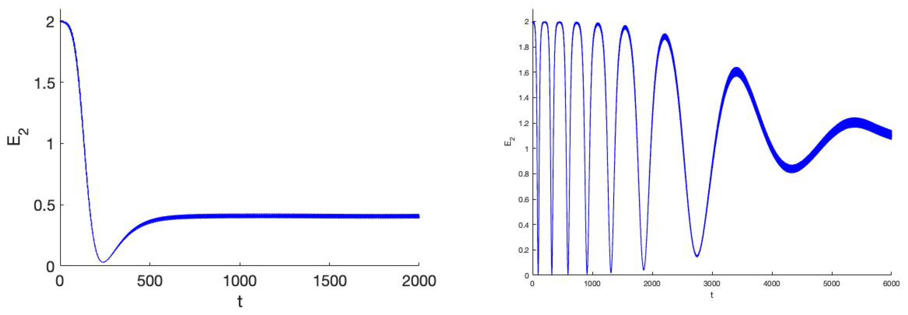
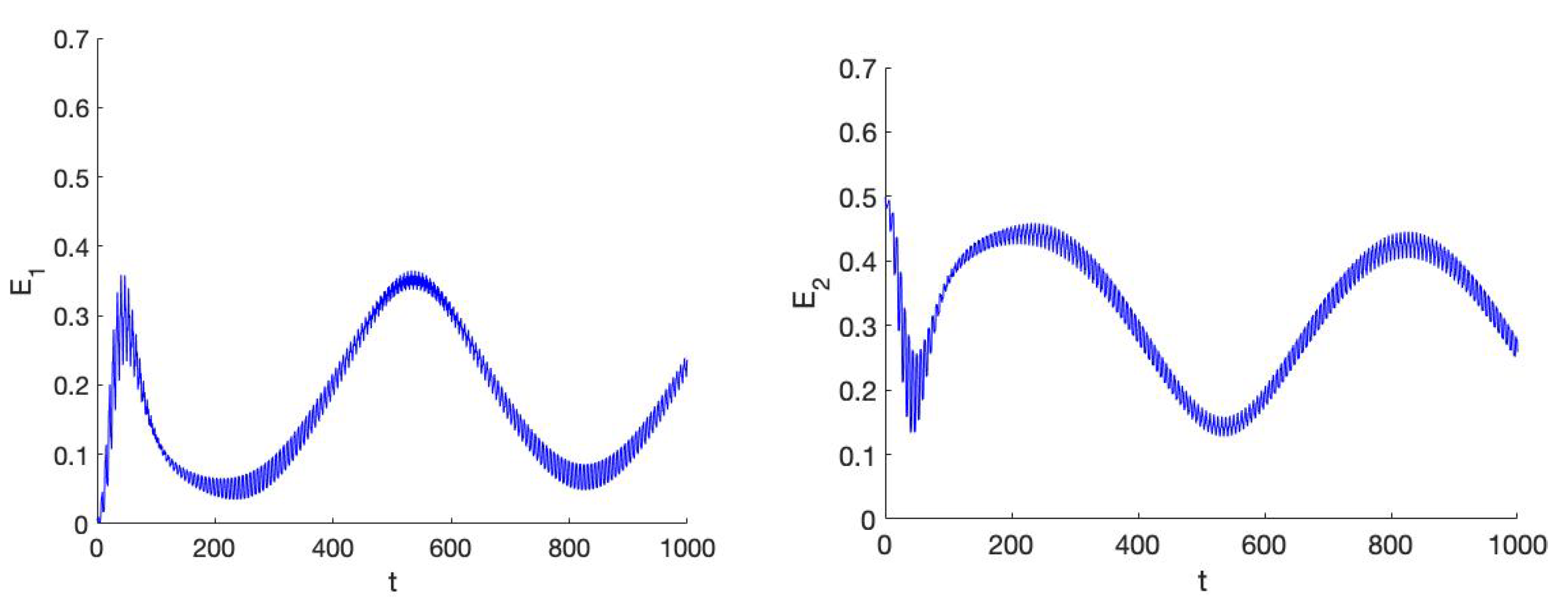
- An interesting consequence arises when considering orbits that change stability during the process of evolution to mirror symmetry. The instability of the normal mode persists at second order but leads to stability in the final stage of mirror symmetry after a time dependent on . The implication is that this will generally produce a drastic change of actions. Another qualitative consequence is that the epicyclic normal mode does not exist in the first stage (time order ) but the normal mode exists in the final stage of mirror symmetry; again we can expect action changes. Similar considerations hold for the unstable out-phase periodic solutions derived before. For illustrations see Figure 1 and Figure 2 and the discussion below. In Figure 1 the corresponding action is not shown; it exchanges energy met the z-mode.
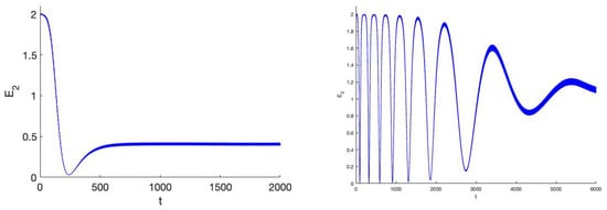 Figure 1. The behaviour of action of system (14) in 2 cases near the z-normal mode; (left and 2000 timesteps and right , 6000 timesteps). We have with initial velocities zero, . After around 600 timesteps the time-dependent interaction vanishes if . In the case it takes more than 6000 timesteps. In both cases the dynamics and velocity distribution has changed considerably by the evolution to mirror symmetry.
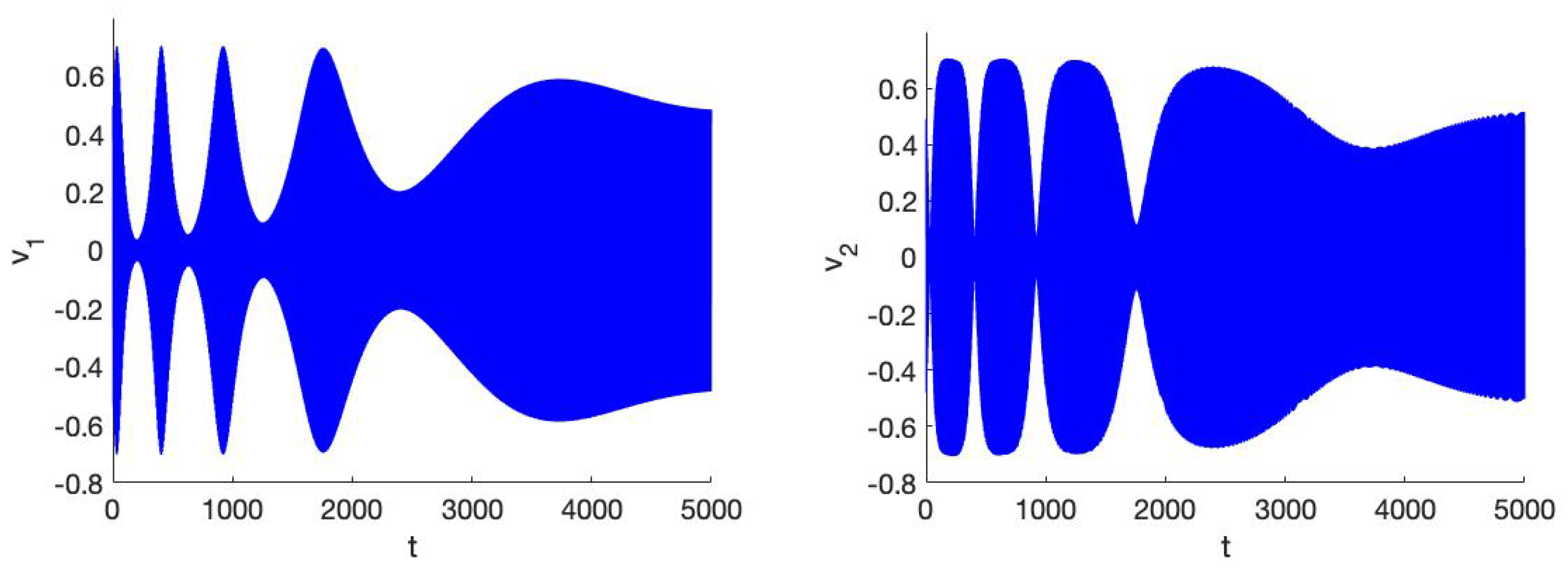
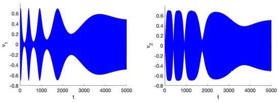 Figure 2. The behaviour of the velocities of system (14) in 1:2 resonance for the case , it takes longer for the time-dependent interaction to vanish. The initial conditions are and initial velocities zero.
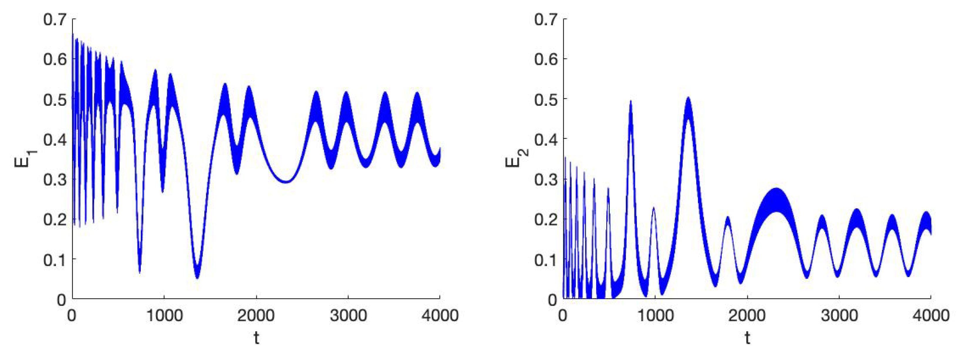
5.3. Consequences for the Distribution Function at the 1:2 Resonance
Suppose we start with a collection of particles (stars) characterised by a distribution function satisfying the Boltzmann equation that is nearly collisionless as it has small dynamical friction added. The system is already in axi-symmetric state but the evolution to mirror symmetry to the galactic plane is still going on. On an interval of time , the first stage of evolution, we have, apart from angular momentum J, two active integrals of motion: and a prominent resonance manifold for each value of the energy described by Equation (23). The family of solutions with constant amplitude (constant to )) on the energy manifold will be stable for combination angle . The distribution function will be a function of the 3 integrals. The velocity distribution and their dispersion will depend on the presence of these integrals.
On intervals of time asymptotically larger than , the primary resonance manifolds described by Equation (23) vanish, they are replaced by the smaller resonance manifolds (of size ) located by the zeros of Equation (27) and . The distribution function will now evolve to a function of the actions but with an initial velocity distribution obtained by the resonance on time intervals . See Figure 1 (left) where so that the symmetric state develops on intervals of time . On an interval of time order there is first a typical 1:2 resonance exchange between the 2 dof after which the dynamics settles at different actions. If we find, as expected, that it takes much longer to settle in a permanent state, see Figure 1. With the choice of the effect of evolution to symmetry is much less.
In Figure 2 we have so that on intervals of size we have still resonant interaction, the symmetric state develops on intervals of size . The exchanges and time evolution are first much more frequent as it takes longer for the asymmetric terms to vanish. Then the system settles at a much lower oscillation amplitude, in a sense experiencing more of its asymmetric past.
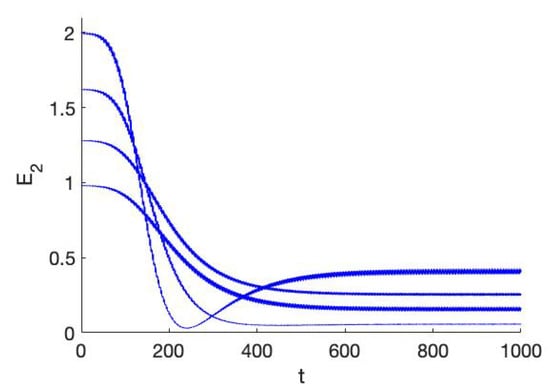
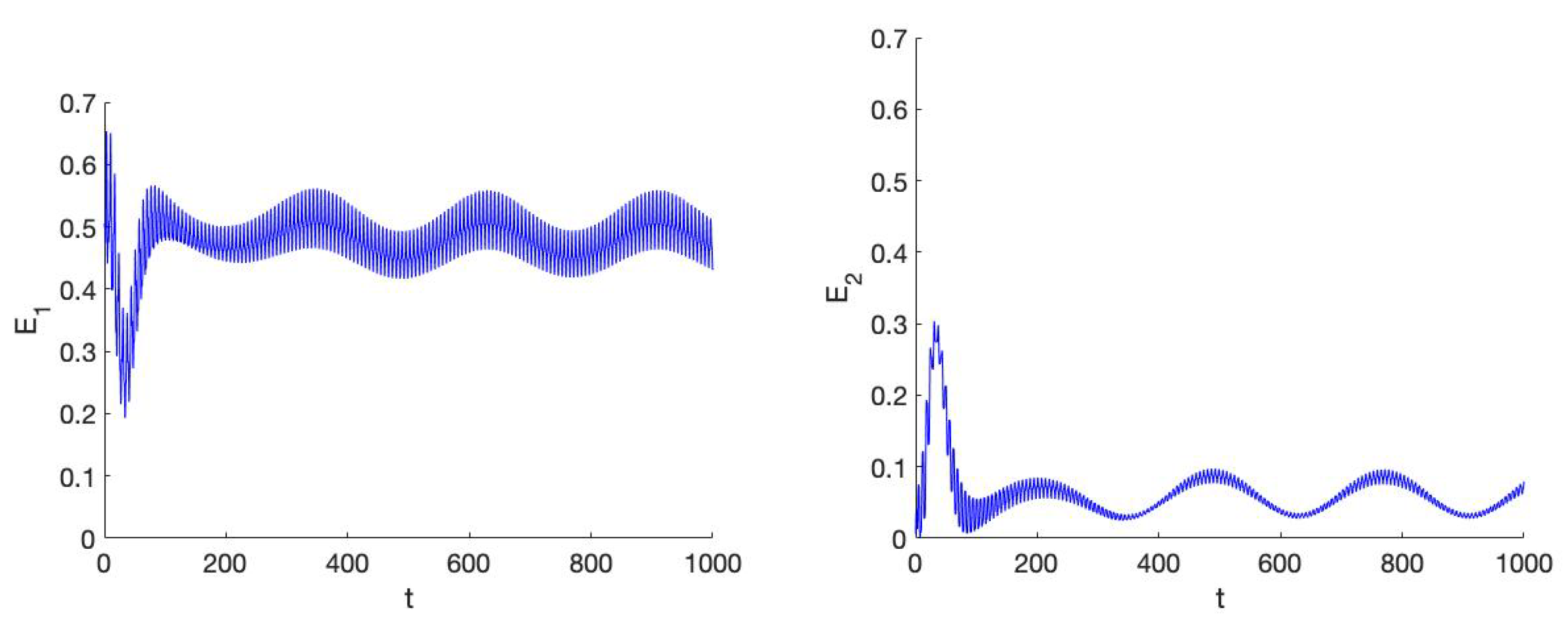
In Figure 3 we show the behaviour (left) near the z normal mode for different values of the energy in the case . Interesting is that starting at the resulting values of are lower than for a few orbits starting at still lower energy. This will be caused by passage of more complicated structures like resonance manifolds in phase-space.
When the system is close to mirror symmetry, we will find for each value of the energy in a resonance manifold a family of tori around the stable periodic solutions, so for varying energy values this will be a 2-parameter family. Outside these resonance manifolds the orbits will move quasi-linearly, only the phases are position dependent.
The choice of , the parameter determining the timescale of destroying the asymmetry of the potential field, together with the energy level will determine the resulting positions and velocities.
6. The 1:3 Resonance
The 1:3 resonance is for Hamiltonian (10) dynamically very different and less interesting. Most of the analysis can be deduced from [9], we will summarise the results. Putting in (10) we find after 2nd order averaging:
The result is quite remarkable as this shows that for the 1:3 resonance the slowly vanishing asymmetry of the potential plays no part for the amplitudes to order 3 in . For the phases we find no asymmetric terms either but nontrivial variations depending on the symmetric potential:
if or the asymmetry plays no significant part. The theory of higher order resonance, see [11] and for extension and examples [4], shows that the combination angle plays a crucial role. The equation for becomes:
Zero solutions of the right-hand side of Equation (30) produce, together with the condition resonance manifolds of size with characteristic timescale for the orbits and motion on the corresponding tori; these estimates follow from the analysis in [4]. With high precision the distribution function will depend on J and the 2 actions.
It is clear that if , system (29) has no nontrivial zeros and so the resonance manifolds of this type are not present.
7. The 1:1 Resonance
If the epicyclic frequency and the vertical frequency are equal or close, the 1:1 resonance becomes important. As shown in Section 3 this happens for instance in the case of a very large mass in the centre of the galaxy. With given by Equation (20) the equations of motion induced by Hamiltonian (10) are:
By averaging system (31) using amplitude-phase coorditates (15) we find that all first order averaged terms vanish. Significant dynamics takes place on a longer timescale so we choose to consider longer time scales. Second order averaging based on [11] produces with the system:
From system (32) we can derive the equation for . The dynamics of the 1:1 resonance turns out to be more complicated than the cases 1:2 and 1:3 as both time-dependent and independent terms are strongly active on intervals of time , see again Section 9. From the equations for the amplitudes we find:
so for the actions we have an adiabatic invariant for system (32):
For bounded solutions invariant (33) is valid for all time with error . System (32) yields approximations for the epicyclic x and the vertical z normal modes. As we shall see, in-phase and out-phase solutions with constant amplitudes or actions exist in general position. For the combination angle we find using actions:
Putting in system (32) we find with and Equation (34) conditions for solutions with constant amplitudes (actions). However, behaviour of constant amplitudes (or actions) is only valid with error on intervals of time ; see for an example Section 7.2.
The solutions of the averaged system to second order with appropriate initial values produce an approximation on an interval of time order of system (16) with but an approximation on an interval of time . The second estimate is a kind of “trade-off” of error estimates valid under special conditions formulated in [12]; see also [11]. It is remarkable that system (32) shows full resonance involving exchange of energy between the 2 dof even when the asymmetric potential terms have become negligible.
A systematic study of the symmetric case () can be found in [9]. The condition determines stationary solutions of the combination angle , it produces conditions on the amplitude and so on the actions (). We summarise from [9] the results for the symmetric, time-independent case :
- The epicyclic normal mode is an exact solution, it is unstable for and .
- The vertical normal mode is obtained from the system (32) as an approximation. It is unstable for .
- The in-phase periodic solutions exist for and are stable for .
- The out-phase periodic solutions exist and are stable for .
We expect the dynamics of the symmetric case to describe the orbits of system (31) on intervals of time larger than . During evolution the in-phase and out-phase solutions are present with constant amplitude and approaching periodicity. The dynamics will after long time be governed by the integrals (35) and (36) producing a complicated velocity distribution and varying actions.
On the long (starting) interval of order system (32) has also 2 integrals. As noted before integral (35) holds for all time .
As the 1:1 resonance occurs in applications and has been studied in many papers we will consider examples in more detail.
7.1. Avoiding Degenerate Cases
Special values of parameters may produce degenerations that produce dynamics that is not typical. We illustrate this by looking for solutions of system (31) of the form with a suitable parameter. This assumption implies a degeneration as it means that there is no exchange of energy between the 2 modes. Substituting this relation into system (31) we find the conditions:
Using 2nd order averaging as in example 12.20 of [13] with we find:
This type of special solutions shows only variation of the phases. Although interesting in itself, we have to avoid the parameter values of conditions (37) when studying more general behaviour. Other parameter values that may lead to degenerations and should be avoided are the bifurcation values of existence and stability of normal modes and other periodic solutions listed in the preceding subsection.
7.2. An Example of Evolution
In Figure 4, Figure 5, Figure 6, Figure 7 and Figure 8 the choice of gives the system stable epicyclic and stable vertical normal modes if we would have the time-independent case. However, our choice of keeps the normal modes but destabilises them; we have . When the time-dependent perturbation has become negligible after roughly 200 timesteps if and 3000 timesteps if , the orbits have moved into general position. The time-independent case will approximate the dynamics after a long initial period of time, the in- and out-phase periodic solutions exist if , the out-phase solutions are stable.

Figure 4.
Left the behaviour of the action of system (31) in 1:1 resonance for the case near the epicyclic normal mode; initial conditions . Parameter values . Right we display the corresponding z behaviour by plotting . It takes around 200 timesteps to settle in the stationary state which is drastically different from the initial state.
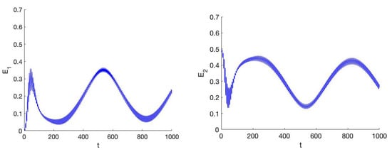
Figure 5.
Left the behaviour of the action of system (31) in 1:1 resonance for the case near the vertical (z) normal mode; initial conditions . Parameter values . Right we display the corresponding z behaviour by plotting . It takes around 200 timesteps to settle in the stationary state which is drastically different from the initial state.
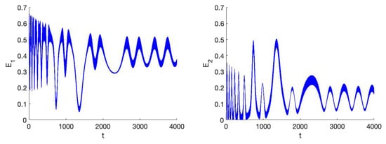
Figure 6.
Left the behaviour of the action of system (31) in 1:1 resonance for the case near the epicyclic normal mode; initial conditions . Parameter values . Right we display the corresponding z behaviour by plotting . It takes around 3000 timesteps to settle in the stationary state which is drastically different from the initial state.
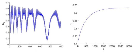
Figure 7.
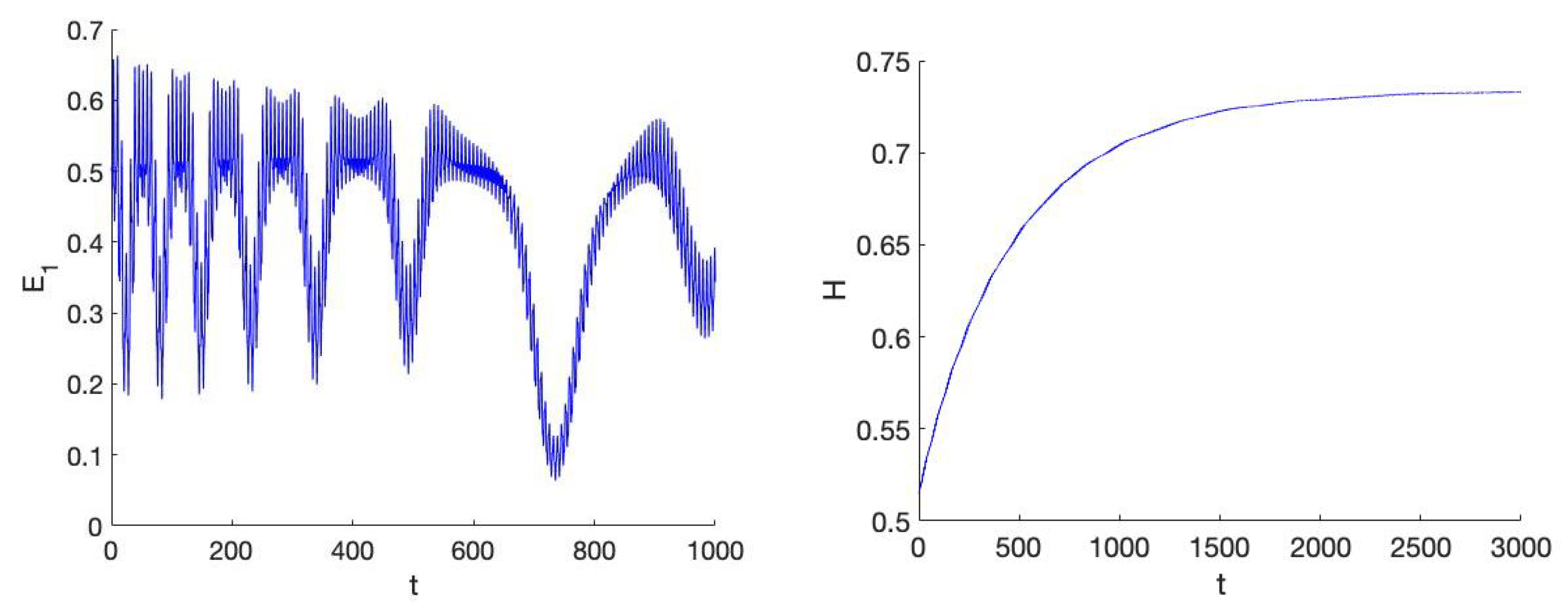
Left an enlargement of of Figure 6 (the 1:1 resonance for the case near the epicyclic normal mode). The initial phase where the asymmetric potential is active takes around 500 timesteps. Right we show the Hamiltonian in this case. It shows monotonic behaviour.
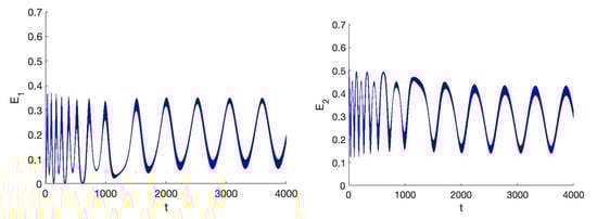
Figure 8.
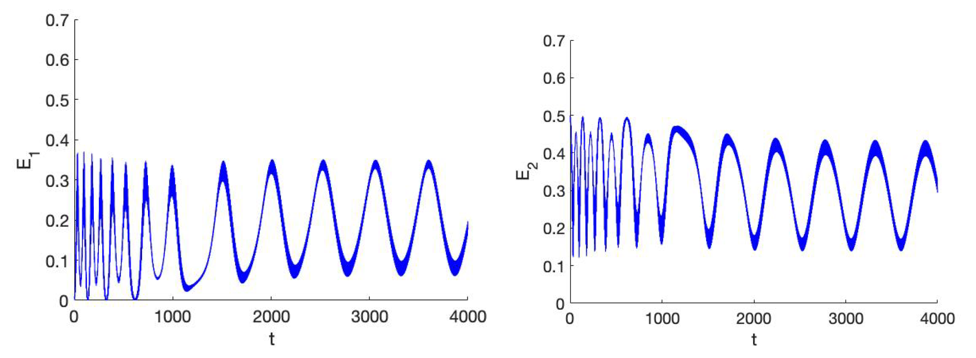
Left the behaviour of the action of system (31) in 1:1 resonance for the case near the vertical (z) normal mode; initial conditions . Parameter values . Right we display the corresponding z behaviour by plotting . It takes around 3000 timesteps to settle in the stationary state which is drastically different from the initial state.
For the actions: we have from system (32):
with . In our example we have .
Solutions with constant amplitude are obtained when putting ; they are valid with error on intervals of time . On these intervals time-dependent terms are important. In our example, the in-phase and out-phase periodic solutions with constant amplitude exist if also for each small value of the energy where averaging-normalisation is valid. They represent, like the normal modes, continuous families of periodic solutions parametrised by the energy. Adding the time-dependent terms destroy the periodicity but these terms become negligible after a long time.
In Figure 4 and Figure 6 we start near the epicyclic normal mode, in Figure 5 and Figure 8 near the vertical normal mode; in both cases the solutions move into general position on tori around periodic solutions. The asymmetric past of the system has changed the overall dynamics drastically, but this depends strongly on the initial phase where the potential is still asymmetric.
The initial phase on intervals of size .
If we will have that changes on this interval, in our example . The adiabatic invariant (33) will be active on an interval of size . As we observe in Figure 6, (enlarged in Figure 9) the initial phase takes around 500 timesteps if . In the initial phase we have for the dynamics:
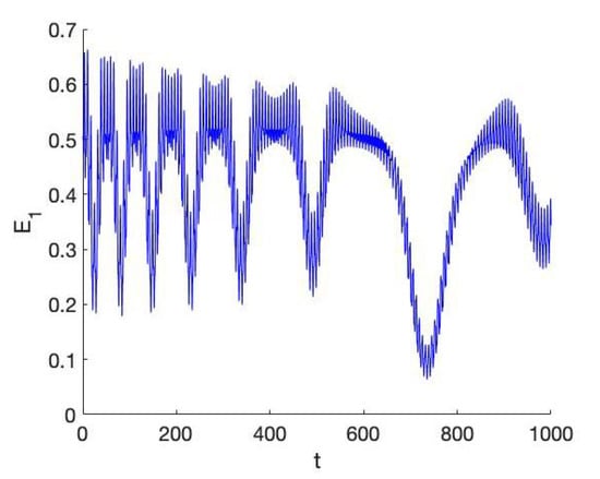
Figure 9.
Enlargement of of Figure 8 (the 1:1 resonance for the case near the epicyclic normal mode). The initial phase where the asymmetric potential is active takes around 500 timesteps.
7.3. Evolution to the Hénon-Heiles Potential
The Hénon-Heiles potential is slightly degenerate as we have to normalise to terms of degree 6 () to obtain structurally stable results, see [14]. There are many details available on this system. If and the system is chaotic but large-scale chaos sets in at , the energy manifold is bounded if . In Figure 10 (left) we present for action close to the chaotic stage. The first 600 timesteps shows irregular motion, then the dynamics settles in motion on tori. The normal forms obtained before will not be valid for these parameter values.
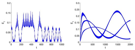
Figure 10.
Left of the Hénon-Heiles system for the case with close to the chaotic stage, . Right the Hénon-Heiles system for the case and for 3 cases: ; we find small oscillations of around a long-time oscillation (increase of produces higher maxima and shorter return times.
8. Conclusions and Discussion
- The resulting dynamics of a rotating axisymmetric galaxy to a state of mirror symmetry with respect to the galactic plane depends on at least three aspects: the local resonance ratio of epicyclic and vertical frequencies, the timescale of evolution to symmetric equilibrium characterised by and the initial phase-space distribution.
- The dynamics of a potential producing locally the 1:2 resonance shows surprisingly that the main effects are described by an approximation. Two adiabatic invariants (approximate integrals) are active, an approximation shows only evolution in the phases. If the evolution takes place with time-like variable the velocities (and corresponding actions) settle quickly at values quite different from the initial ones. Evolution with time-like variable produces strong interactions before settling in a final symmetric state; see Figure 1, Figure 2 and Figure 3.
- For the 1:3 resonance the evolution to a symmetric state of mirror symmetry does hardly affect the final dynamics. The distribution function for orbits in phase-space depends to high approximation on the quadratic integrals . See Section 5 for details.
- The 1:1 resonance plays a natural part in galactic models, it turns out to have interesting dynamics. An approximation on intervals of time is in this case equivalent to an approximation on intervals of time . We find 2 adiabatic invariants that rule the dynamics on intervals of time . If the evolution to mirror symmetry takes place with timelike variable the dynamics starting near normal modes changes to rather strong exchanges of energy between the modes, see Figure 4 and Figure 5. For evolution with timelike variable this effect is much stronger, see Figure 6, Figure 7 and Figure 8.
- An interesting conclusion is that in the final stage of evolution to mirror symmetry with respect to the galactic plane of a rotating axisymmetric galaxy their position in phase-space depends strongly on its asymmetric past. The epicyclic and vertical velocity dispersions will be different and are tied in with the resonance-dependent adiabatic invariants.One of the implications is that a statistical mechanics description of systems of particles in near-equilibrium and held together by mainly gravitational forces can not be understood without considering earlier evolutionary states.
9. A Synopsis of Averaging Theorems
Averaging methods were used as a formal method in the 18th century. In the first half of the 20th century proofs and extensions of the methods were developed in France and in the Sowjet-Union. For a brief historical survey see appendix A of [11]. Sometimes the methods are referred to as averaging-normalisation as there is a definite relation with normal form methods, see [11] chs. 9–13.
Consider initial value problems of the form
with given and a small parameter, . To analyse this initial value problem as a perturbation problem makes sense if we have knowledge about the system for . Using this knowledge and applying variation of constants one can often obtain a system of slowly varying variables of the form where a T-periodic vector field plays a part. Consider explicitly the T-periodic vector fields and the slowly varying ODE:
With and twice continously differentiable in a bounded domain D in , continuously differentiable in t. Suppose in addition that:
where x is kept constant during integration. We will call the terms represented by non-resonant to first order. We use the near-identity transformation:
Such transformations were also used in [12]. As the vector field is t-periodic with average zero, is bounded in D by a constant independent of . Substituting with Equation (45) in ODE (44) we have:
We expand . and find:
I is the unit matrix, the matrix has a bounded inverse, so that:
where the terms can be computed explicitly. The procedure removes the non-resonant terms from the right-hand side of Equation (44); this is useful if we are able to perform analysis on the resonant part with explicit slow time as in Section 3. In our models a second small parameter plays a part. This is handled in various ways. We can assume a relation between and . In our models we have that occurs in the combination so we can introduce the independent slowly varying variable by .
In formulating next a number of theorems we omit detailed assumptions regarding smoothness and dimensions.
Theorem 1.
Consider the initial value problem
with n-dimensional vector field T-periodic in t. Introduce the average
then we have for the solutions of the initial value problems (47) and
on time intervals of order .
For a proof and more detailed conditions see [11] Chapter 4.2.
In many problems a second order approximation is necessary for qualitative and quantitative reasons.
Theorem 2.
Consider the Jacobian matrix and the vector field
Introduce vector field
Average over t producing and consider the initial value problems (47) and
Then we have on time intervals of order .
For a proof and more detailed conditions see [11] Chapter 4.5.
A useful extension was given in [12], see also [11] Chapter 2.9. It is:
Theorem 3.
Consider the formulation of theorem 2 and in addition assume . Then we have that on time intervals of order .
The theory of higher order resonance for 2 dof Hamiltonian systems was started in [15]. It was extended in [4], see for a summary [11] Chapter 10.6.4. The theory is technically too involved to give a summary here. We mention two typical aspects. On studying 2 dof systems with basic resonance, we have a higher order resonance if ; a lower order resonance is also described by the theory of higher order resonance if there are certain degenerations in the averaged system (this happens in our paper for the 1:2 and 1:3 resonance). In general the dynamics in phase-space is characterised by large domains without much interaction between the two degrees of freedom whereas interaction takes place in resonance manifolds with a fractal dimension in .
Funding
This research received no external funding.
Acknowledgments
System (25) was helpfully computed by Taoufik Bakri using Mathematica.
Conflicts of Interest
The authors declare no conflict of interest.
References
- Roseau, M. Vibrations Nonlinéaires et Théorie de la Stabilité; Springer: Berlin/Heidelberg, Germany, 1966. [Google Scholar]
- Verhulst, F.; Huveneers, R. Evolution towards Symmetry. In Regular and Chaotic Dynamics; Moser, J., Kozlov, V.V., Eds.; MAIK Nauka/Interperiodica: Moscow, Russia, 1998; Volume 3, pp. 45–55. [Google Scholar]
- Huveneers, R.J.A.G.; Verhulst, F. A metaphor for adiabatic evolution to symmetry. SIAM J. Appl. Math. 1997, 57, 1421–1442. [Google Scholar]
- Tuwankotta, J.M.; Verhulst, F. Symmetry and resonance in Hamiltonian systems. SIAM J. Appl. Math. 2000, 61, 1369–1385. [Google Scholar]
- Ollongren, A. Three-Dimensional Galactic Stellar Orbits. (Thesis Leiden, 1962). Bull. Astr. Inst. Neth. 1962, 16, 241–296. [Google Scholar]
- Binney, J.; Tremaine, S. Galactic Dynamics; Princeton Series in Astrophysics, Princeton UP 3rd Printing; Princeton University Press: Princeton, NJ, USA, 1994. [Google Scholar]
- Dehnen, W.; MacLaughlin, D.E.; Sachania, J. The velocity dispersion and mass profile of the Milky Way. Mon. Not. R. Astron. Soc. 2006, 369, 1688–1692. [Google Scholar] [CrossRef] [Green Version]
- Brown, W.R.; Geller, M.J.; Kenyon, S.J.; Diaferio, A. Velocity dispersion profile of the Milky Way halo. Astron. J. 2010, 139, 59–67. [Google Scholar] [CrossRef]
- Verhulst, F. Discrete symmetric dynamical systems at the main resonances with applications to axi-symmetric galaxies. Phil. Trans. R. Soc. Lond. 1979, 290, 435–465. [Google Scholar]
- Henon, M.; Heiles, C. The applicability of the third integral oi motion: Some numerical experiments. Astron. J. 1964, 69, 73–79. [Google Scholar] [CrossRef] [Green Version]
- Sanders, J.A.; Verhulst, F.; Murdock, J. Averaging Methods in Nonlinear Dynamical Systems, 2nd ed.; Applied Mathematical Sciences 59; Springer: New York, NY, USA, 2007. [Google Scholar]
- van der Burgh, A.H.P. On the asymptotic approximations of the solutions of a system of two non-linearly coupled harmonic oscillators. J. Sound Vibr. 1976, 49, 93–103. [Google Scholar] [CrossRef]
- Verhulst, F. Methods and Applications of Singular Perturbations; Springer: New York, NY, USA, 2005. [Google Scholar]
- Gustavson, F.G. On constructing formal integrals of a Hamiltonian system near an equilibrium point. Astron. J. 1969, 71, 670–686. [Google Scholar] [CrossRef]
- Sanders, J.A. Are higher order resonances really interesting? Celest. Mech. 1977, 16, 421–440. [Google Scholar] [CrossRef]


Publisher’s Note: MDPI stays neutral with regard to jurisdictional claims in published maps and institutional affiliations. |
© 2021 by the author. Licensee MDPI, Basel, Switzerland. This article is an open access article distributed under the terms and conditions of the Creative Commons Attribution (CC BY) license (https://creativecommons.org/licenses/by/4.0/).