A Global Search Method for Inputs and Outputs in Data Envelopment Analysis: Procedures and Managerial Perspectives

Abstract

Effective decision-making techniques are essentially dependent on the capacity to balance (symmetry) requirements and their fulfilment, that is, the capacity to accurately identify a collection of factors that have the greatest influence on performance. Data envelopment analysis (DEA) is a useful nonparametric method in operations research for performance estimation by measuring the efficiency scores of the decision-making units. In this paper, we develop a global search method (GSM) for selecting the key input and output variables in DEA models. The GSM measures the effects of variables with respect to the efficiency scores directly, i.e., by considering the average change when a variable is added or removed from the analysis. It aims to produce DEA models that include only the key variables with the largest impact on the results. The effectiveness of the GSM is demonstrated using a case study from 15 US banks, with the results analyzed and discussed. The outcomes indicate that the GSM yields useful insight for decision-makers to make informed decisions in undertaking their problems.

1. Introduction

Data envelopment analysis (DEA) has been regarded as a powerful technique to select and combine models for general k-class classification problems in machine learning [1,2]. The application of DEA as an ensemble for classifiers in machine learning is inspired by the ROCCH (receiver operating characteristics convex hull) [3] which was mainly for the two-class classification problem. DEA was first proposed by [1] to construct ensembles for classifiers and they showed that DEA identified a convex hull that is identical to that of ROCCH for a classification problem with two classes. From then onwards, DEA has been utilized as an ensemble of classifiers that can be applicable to problems with multiple classes [2]. Baumgartner and Serpen [4] had further shown that integrating multiple base classifiers into an aggregated outcome (or ensemble) has turned out to be an efficient strategy for achieving superior prediction performance.

The underlying fundamentals of DEA is based on a nonparametric approach that addresses the issue of determining the efficiency of various “decision-making units” (DMUs) based on how inputs are converted into outputs [5]. A DMU is rated as fully efficient (100%) if and only if the performance of other DMUs does not show that some of its inputs or outputs can be improved without worsening some of its other inputs or outputs [6]. DEA, which is extensively used to investigate a wide range of industries [7,8] and has lately been implemented in the big-data toolbox [9], employs mathematical programming to discover efficient DMUs, which constitute an efficient frontier. The efficiency score in DEA analysis highly relies on the set of input and output variables used in the efficiency measure. Hence, if DEA is to be fully utilized in evaluating as many different classifiers as possible, inputs and outputs variables selection in a DEA model is critical. We therefore expect to address this problem of DEA by developing a global search method (GSM) for optimizing variables selection.

The contributions of this paper are as follows. Firstly, this study enhances DEA for efficiency measurement which is the key concept for performance. Secondly, this paper generates a searching algorithm for variables selection that include variables with the largest impact on the DEA results, in which the algorithm is grounded on optimization approach. Finally this study yields useful managerial insights for decision-makers to make reliable judgements and to be used as guidelines to adjust or balance (symmetrize) their strategies and needs with proper allocation of resources.

This paper is organized as follows. Section 2 presents the literature on variables selection in DEA. Section 3 presents the methodology of the global search method (GSM). In Section 4, we illustrate this method using sample datasets and discuss the new managerial insights resulting from the GSM. In Section 5, further illustration and validations on GSM are presented using two established numerical examples and a case study on US banks. Concluding remarks are presented in Section 6.

2. Past Research on Variables Selection in DEA

It is very important to select the potential variables to be considered in a DEA model. In general, any resource used by a DMU should be treated as an input variable, and the outputs come from the performance and activity measures when the DMU converts its resources to produce products or services. However, how to choose the right input and output variables has attracted only little attention in the existing literatures. Most of the existing studies on DEA simply treat the input and output variables as “givens” and then go on to deal with the analysis. As it was until 1989, Golany and Roll [10] gave an overall view of DEA that should focus on the choice of variables in addition to the methodology itself. The attention to variable selection is important because the increasing number of input and output variables will constrain the weights assigned to the variables, and the analysis of the results will become less discerning. Jenkins and Anderson [11] applied regression and correlation analysis to identify which variables were to be omitted from the DEA model on the basis of the minimum loss of information. Information was related to the variance of an input or output variable about its mean value. Morita and Avkiran [12] proposed a statistical approach to find an optimal inputs/outputs combination by using diagonal layout experiments.

While there is no consensus on how best to select the variables, many guidelines have been proposed in the literature suggesting limiting the number of variables relative to the number of DMUs. In general, a rough rule of thumb in the envelopment model of DEA is to choose n (= the number of DMUs) equal to or greater than max{m × s, 3 × (m + s)}, where m and s are the inputs and outputs variables respectively (see [13] for more details). The challenge in DEA is to find a ‘parsimonious’ model, using as many input and output variables as needed but as few as possible. The greater the number of input and output variables in a DEA, the higher is the dimensionality of the linear programming solution space, and the less discerning is the analysis [11].

Several methods have been proposed that involve the analysis of correlation among the variables, with the goal of choosing a set of variables that are not highly correlated with one another. These methods purport those variables which are highly correlated with existing model variables are merely redundant and should be omitted from further analysis. Unfortunately, Nunamaker [14] figured out that these methods yield results which are often inconsistent in the sense that removing variables that are highly correlated with others can still have a large effect on the analysis results. In addition, a parsimonious model typically shows generally low correlations among the input and output variables, respectively [15,16]. Appa et al. [17] proposed a method of adding variables to the DEA model one at a time. They claimed that high statistical correlation was an indicator that a particular variable influenced the performance. The authors did note that the observation of high statistical correlation alone was not sufficient. After that, Jenkins and Anderson [11] applied regression and correlation analysis to identify which variables were to be omitted from the DEA model on the basis of the minimum loss of information. Information was related to the variance of an input or output variable about its mean value. Their statistical approach using partial correlation analysis resulted in a measure of information contained in each variable. The authors found that the DEA results could vary greatly according to which highly correlated variables were included or omitted from the DEA model.

At the same time, some investigations start to evaluate the marginal impact on the efficiencies of an adding or omitting a given variable, and focusing on evaluating the statistical significance of the changes in the efficiencies [18]. Another statistical approach for variable selection was developed by [19]. They focused on the inner models which data differed in one single input or output variable. They evaluated a reduced DEA model without one particular variable, and an extended model that included one variable. Then, for each DMU, the efficiency scores were calculated under both the reduced and extended model. A statistical test was conducted to determine the significance of the efficiency contribution of the particular variable being evaluated. Amirteimoori et al., [20] developed an approach that aggregates selected high correlated inputs/outputs to reduce the total number of variables and increase the degree of discrimination. While Ref. [21] pointed out that such approach is unstable due to the epsilon is not unique, they have improved the approach to only one step iteration.

In contrast to correlation based methods, which look at the input and output variables before applying DEA to determine the likely effect on the efficiency scores after the application of DEA, other approaches examine directly the effect on the efficiency scores when the input and output DEA variables are changed. The initial model was compared with those of a new model in which one additional variable was added. Ref. [22] developed a “stepwise” selection approach to examine the changes in the efficiencies as variables are added and removed from the DEA model, often with a focus on determining when the changes in the efficiencies can be considered statistically significant.

In addition, their approach has not considered the rule of thumb, and each selection step is only based on the minimum efficiency change with the last step that is just local optimal—it may not lead to the optimal global decision. Toloo et al. [21] developed selecting models of performance measures in DEA; their models applied the rule of thumb to keep the balance between the number of DMUs and the number inputs/outputs by solving a series of mixed-integer linear programming (MILP) model. However, whether viewing from individual DMU or aggregate, such a model is still unable to determine exactly which variables should be selected, because they consider those performance measures “appear the most often” and take the risk of losing important managerial information.

In this study, we advance the work on variable reduction methods in DEA by formalizing a “global search method (GSM)” for the selection process, and examine the managerial insights gained from using this method. Our proposed GSM measures the effect of influence of variables directly on the efficiencies by considering their average change as variables are added or removed from the analysis. This method is intended to produce DEA models that include only those variables with the largest impact on the DEA results. Moreover, it is useful for models which do not have sufficient number of DMUs and violate the rules of DEA. This can happen in niche classifications (e.g., markets) where the number of comparable DMUs is few, or new classifications (e.g., industries) where the number of measures far exceeds the total number of DMUs. This method is easy to understand, and therefore, it is useful to managers and decision-makers, as it does not need extensive additional calculations.

3. A Global Search Method for Selecting Variables in DEA

We begin by describing the procedures of GSM. The GSM aims to optimize the number of DEA variables and to find the key input and output variables which influence the efficiency scores. We now explain in detail the GSM procedure for effective omission of DEA inputs and outputs.

This approach starts by considering all possible combinations of input and output variables in the DEA model. Assume an original DEA model that has m inputs and s outputs, the total number of DMUs is n. The rule of thumb in [13] provides a guidance for determining a numerical relation between the number of DMUs and number of inputs/outputs, i.e.,

n ≥ max{3(m + s), m × s}

(1)

Set a₁ input variables and a₂ output variables are planned to be kept in the model, where $a_1,a_2\in N*$. The selection procedure will be divided into N cases that depends on the condition of formula (1).

$$N=\{\begin{array}{l}card(\{(a_1,a_2)|a_1+a_2\le \frac{n}{3}\}),if3(m+s)\ge ms\\ card(\{(a_1,a_2)|a_1{a}_2\le n\}),if3(m+s)<ms\end{array}$$

(2)

where card(A) denotes to count the number of elements in a set A. For each case I, where I = {1, 2, 3, … , N}. N_I represents the number of possible combinations of inputs and outputs, where:

$$N_I=\left(\begin{array}{c}m\\ a_1\end{array}\right)*\left(\begin{array}{c}s\\ a_2\end{array}\right)$$

(3)

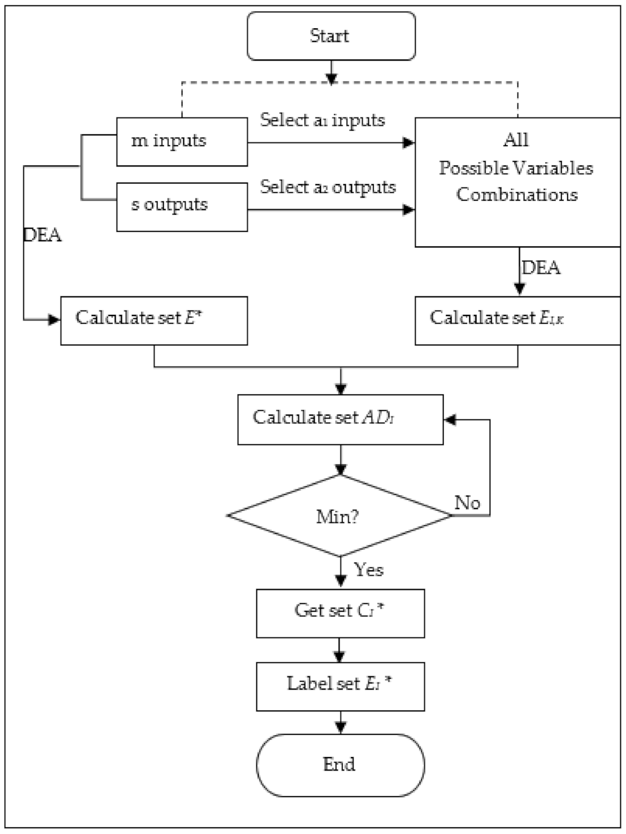
The algorithm for selection procedure is conducted by the following steps.

• Step 1: Run the original DEA model that includes the full set of m input variables and s output variables. Record the efficiency scores of each DMU for this run (set $E^{*}$).
• Step 2: Run a set of k = 1, ... , N_I DEA analyses, keep setting a₁ input variables and a₂ output variables at a time in each run. For each analysis, record the efficiency scores of each DMU (set $E_{I,k}$) for all k runs.
• Step 3: Calculate, for each DMU, the average differences AD_I in the respective DMU efficiency scores by

  $$A{D}_I=\frac{1}{n}\left(E^{*}-E_{I,k}\right)$$

  (4)
• Step 4: Choose the optimal variables combination C_I * to be kept by selecting the variable with the minimum average difference in the efficiency scores from above.

  C_I* = min {AD_I}

  (5)
• Step 5: For the variables selected to be kept, label the DEA results E_I* based on the efficiency scores of the DMUs for the remaining input and output variables.

Through steps 1 to 5, the optimal variables combination C_I* and the corresponding DEA results E_I * are worked out by searching through all the variables’ combinations for case I, which means the optimal a₁ input variables and a₂ output variables have been selected to remain in the model with the minimum average difference in the efficiency scores. Figure 1 shows the flow chart of the GSM algorithm for case I.

Then, for all N cases, calculate all the possible efficiency scores under all combinations of the input and output variables by comparing the changes in efficiency with that of the original model. The total number of possible combinations of the input is:

$$T_c={\displaystyle \sum }_{I=1}^N{N}_I$$

(6)

Theoretically, the method reiterates until only one input and one output variable remain in the model (i.e., for case I = 1). From the practical viewpoint, how many cases should be evaluated depends on the decision criterion to create a parsimonious DEA model. It should also be noted that the GSM procedure does not rely on the particular form of the DEA model. This procedure can be used with either CRS or VRS, or with static or stochastic data, as long as the same model is used consistently in all steps. The complexity analysis of this method is attached in Appendix A.

4. Results

The proposed GSM of DEA variables can easily be demonstrated by using an example. We consider the data sets from eighteen logistics companies (as shown in

Table 1. Data of 18 logistics companies.

DMU	I1	I2	I3	I4	I5	I6	O1	O2	O3
DMU1	7,173,039	4,665,546	2,220,173	11,430,109	11,000	1,076,631	815,161	12,245,269	577,488
DMU2	153,707	145,476	7181	7277	280	2194	905	8182	4457
DMU3	939,409	902,449	36,960	290,085	18	32,467	415,204	705,289	379,699
DMU4	493,906	307,173	147,059	517,766	1549	37,473	17,141	534,907	26,262
DMU5	35,333	25,084	9826	22,173	97	4559	1912	24,085	1441
DMU6	466,368	396,445	70,260	530,222	493	24,630	39,389	569,611	25,323
DMU7	98,994	66,529	32,388	112,552	83	16,247	9994	122,546	9641
DMU8	719,315	505,479	192,045	293,421	2288	162,686	142,624	436,045	150,716
DMU9	638,625	528,936	72,211	173,320	1392	32,952	17,494	190,814	15,970
DMU10	466,216	334,537	125,959	225,573	1445	46,286	27,270	252,843	21,727
DMU11	213,201	166,998	38,928	134,985	563	27,054	28,037	163,022	16,580
DMU12	2,187,708	2,117,114	69,256	257,920	371	29,239	350,222	608,142	481,361
DMU13	74,547	69,426	5518	67,645	1540	18,799	6234	73,879	4441
DMU14	130,826	94,929	35,848	227,195	276	15,628	2880	230,075	2418
DMU15	522,852	232,016	266,412	222,264	762	22,885	9358	231,622	12,690
DMU16	305,799	232,079	69,433	277,171	551	13,413	10,697	287,868	8080
DMU17	27,951,845	25,189,736	2,700,867	8,688,422	8916	909,224	2,510,523	11,198,945	2,861,949
DMU18	930,044	748,004	163,564	492,289	573	33,756	65,324	557,613	35,763

), with the labels of DMU1 to DMU18. The data set contained information of six input variables and three output variables. In this case, the inputs are the following operations indicators.

• I1: total asset
• I2: total capital
• I3: total current liabilities
• I4: total operating expenses
• I5: no. of employees
• I6: selling, general & administrate

The outputs are the following variables:

• O1: operating income
• O2: net sales or revenues
• O3: net profit

4.1. Search the Best Combination in All Possible Cases

In this conciliation, first we ignore the rule of thumb and let N = 8, try to consider all possible combinations of input and output variables in the DEA model and run the GSM model with all cases from step 1 to step 5. Figure 2 shows the trend of average change of efficiency with number of omitted variables. It indicates that as the number of variables decreases, the average of the efficiency change will increase.

Table 2. Optimal combinations in all possible cases.

No. of Kept Variables	Inputs	Outputs	Average Efficiency Change
2	I6	O2	0.3107
3	I2	O2, O3	0.2769
	I6, I4	O1	0.0406
4	I2	O1, O2, O3	0.2718
	I1, I6	O1, O3	0.0389
	I1, I4, I5	O1	0.0169
5	I2, I3, I4, I6	O2	0.0053
	I2, I4, I6	O2, O3	0.0152
	I2, I4	O1, O2, O3	0.0486
6	I2, I4, I6	O1, O2, O3	0.0152
	I2, I3, I4, I6	O2, O3	0.0036
	I1, I2, I4, I5, I6	O1	0.0017
7	I2, I3, I4, I6	O1, O2, O3	0.0117
	I1, I2, I3, I4, I6	O1, O3	1.04E-09
	I1, I2, I3, I4, I5, I6	O2	0.0017
8	I1, I2, I3, I4, I6	O1, O2, O3	9.94E−10
	I1, I2, I3, I4, I5, I6	O2, O3	9.63E−10
9	I1, I2, I3, I4, I5, I6	O1, O2, O3	0

shows the optimal combinations in all possible cases. As for managers, the GSM model not only gives a method of efficiency analysis for decision-making, but also gives alternative options even the number of variables are determined. When examining which of the input and output variables can be kept and the effect on the previously efficient DMUs as they do, provides valuable managerial information. We can also see the output variable “net sales or revenues” has vital effect on the analysis, because, among all the optimal cases, such a variable has always been kept and never been omitted.

4.2. Search the Best Combination under the Rule of Thumb

In this sample, m = 6, s = 3, and n = 18. By applying the rule of thumb, here 3(m + s) = 27, ms = 18. Hence we have

$$n<\max \left\{3(m+s),ms\right\}=3(m+s)$$

(7)

This indicates that the number of inputs/outputs should be omitted to match the condition in (1). Denote a₁ input variables and a₂ output variables will be kept, then it will match

$$(a_1+a_2^{})\le \frac{n}{3}=6,\mathrm{where}{a}_1,a_2\in N*$$

(8)

Therefore, the total optimal number of input/output variables should be no more than 6. Here, if the manager chose six variables of inputs and outputs to keep, this indicates that three variables need to be omitted from total nine inputs/outputs variables. Considering that at least one input and one output should be kept in normal DEA model, and then the possible cases are shown in the following

Table 3. Possible cases of combinations with six variables.

Cases	No. of Inputs (a1)	No. of Outputs (a2)	No. of Combinations
Case1	5	1	18
Case2	4	2	45
Case3	3	3	20

.

In Table 3, for each case, the number of combinations can be calculated by (3). By using the GSM model to do the analysis, the best combination for each case can be easily figured out by comparing the efficiency scores with the original DEA model. As a result, the optimal input variables and output variables have been selected to remain in the model with minimum average difference in efficiency scores.

Table 4. Optimal combinations with six variables.

Cases	Inputs	Outputs	Average Efficiency Change
Case1	I2, I3, I4, I5, I6	O2	0.0017
Case2	I2, I3, I4, I6	O2, O3	0.0036
Case3	I2, I4, I6	O1, O2, O3	0.0152

shows the optimal combination for each case with six variables.

From Table 4, we can find that the combination (I2, I3, I4, I5, I6 and O2) in Case 1 shows the minimum average difference in efficiency scores and hence it is selected as the optimal combination when six variables are selected to be remained. This is due to about 99.83% of the information has been kept after omitting three variables. It means that the input variable “total assets” and output variables “operating income” and “net profit”, which have less contribution to the efficiency scores, could be omitted with a minimum loss of information and no change in DEA scores.

4.3. Find the Key Input and Output Variables

The GSM model can also be used to identify the key variables i.e., the factors that play a significant role in the company’s operations. Identification of key variables is important to managers because this can help them focus on the primary issue of the company. In Table 2, I4 and O2 are identified as the key input and key output; this is because, after the omission of the other variables, the remaining two variables can still keep about 68.93% (where the average efficiency change is 31.07%) of information from the original model with nine variables. However, in most applications this modest change in efficiencies is outweighed by the gains that result in developing a more parsimonious model.

5. Further Illustration and Validations

In this section, the proposed GSM method is further tested and validated using two established numerical examples then followed by a case study. The examples from [11,22] are used here.

5.1. Example 1: Compared with Partial Correlation in Jenkins and Anderson

We begin with a simple exercise using the CCR-I primal model and compare our results with Jenkins and Anderson [11]. In

Table 5. Data for Example 1.

DMU	I1	I2	I3	I4	I5	I6	O1	O2
A	1.5	2.7	70	2.3	1.8	3.3	85	82
B	0.5	0.2	70	1.5	1.1	0.5	96	93
C	2.5	2.6	75	2.2	2.4	3.2	78	87
D	1.8	1.5	75	1.8	1.6	2.3	87	88
E	0.9	0.4	80	0.5	1.4	2.6	89	94
F	0.6	0.2	80	1.3	0.9	2.8	93	93
G	1.4	0.6	85	1.4	1.3	2.1	92	91
H	1.7	1.7	90	0.3	1.7	1.8	97	92

, there are six inputs, two outputs and only eight DMUs.

In order to compare with the method of partial correlation in [11], we omitted the same number of input variables and kept all outputs.

Table 6. The results of GSM model and partial correlation.

No. of Input Variables	GSM		Partial Correlation
	Inputs Kept	E*	Inputs Kept	E*
2	I3, I5	0.005	I1, I3	0.063
3	I3, I4, I5	0	I1, I3, I6	0.063
4	I2, I3, I4, I5	0	I3, I4, I5, I6	0
5	I1, I2, I3, I4, I5	0	I2, I3, I4, I5, I6	0

shows the results of GSM and Jenkins and Anderson’s [11].

From Table 6, we can see the advantage of the GSM model with less efficiency change. If considering two input variables to be kept, the GSM model selects I3 and I5, the partial correlation model selects I1 and I3. However, the GSM analysis shows that if I3 and I5 are to be kept as to retain as much information as possible (measured by average efficiency change), I3 and I5 are the best pair to be kept. The most surprising result is perhaps the choice of variables to keep, which is certainly not accurate from the partial correlation, and how much information is retained by a judicious choice of fewer variables. The partial correlation is indirectly related to the resulting changes in efficiencies, while the GSM model can retain as much as information when choosing the same number of input variables.

5.2. Example 2: Compared with Wagner and Shimsak

In this section, we conduct a further analysis by comparing our GSM model with other related variables selection methods, i.e., stepwise [22] and selective measures [21]. Using the data provided earlier in Table 1 above, we obtain the following results.

Table 7. Results of GSM and Stepwise.

No. of Variables to Be Kept	GSM			Stepwise			Improved by (%)
	Input Kept	Output Kept	E*	Input Kept	Output Kept	E*
2	I6	O2	0.302	I4	O2	0.304	0.13%
3	I1, I6	O1	0.197	I2, I4	O2	0.290	9.21%
4	I1, I4, I5	O1	0.174	I2, I4, I6	O2	0.288	11.48%
5	I1, I4, I5	O1, O3	0.173	I2, I3, I4, I6	O2	0.288	11.49%
6	I1, I2, I4, I5, I6	O1	0.217	I2, I3, I4, I5, I6	O2	0.288	7.10%
7	I1, I2, I3, I4, I5, I6	O2	5.45E−16	I1, I2, I3, I4, I5, I6	O2	5.45E−16	0.00%
8	I1, I2, I3, I4, I5, I6	O2, O3	1.86E−16	I1, I2, I3, I4, I5, I6	O2, O3	1.86E−16	0.00%
Average	-	-	-	-	-	-	5.63%

shows the results of GSM and stepwise. As a general view, GSM model is able to choose the more important variables with less efficiency change, and the results of GSM have 5.63% improvement compared with stepwise model. If we want to choose the ‘core’ variable of the DEA model, which means to select one representative input and output variable with least information lost. The GSM model selects I6 and O2 with average efficiency change of 0.302, which is less than 0.304 from the stepwise method that chooses I4 and O2. In addition, the GSM method can provide valuable and accurate managerial information to the decision-maker that is not available from traditional DEA analysis.

To compare with selective measures method [21], for instance now, here if managers choose to keep five input/output variables, then the results are shown in

Table 8. GSM model vs other methods.

DMU	GSM Model			Step-Wise	Selective Measures	E*
	Variables to Be Kept
	I2, I3, I4, I6, O2	I2, I4, I6, O2, O3	I2, I4, O1, O2, O3	I2, I3, I4, I6, O2	I2, I4, I5, I6, O2	All
DMU1	1.00000	1.00000	1.00000	1.00000	1.00000	1.00000
DMU2	0.46245	0.46281	0.46281	0.46245	0.46245	0.46281
DMU3	1.00000	1.00000	1.00000	1.00000	1.00000	1.00000
DMU4	0.93322	0.93322	0.88721	0.93322	0.93322	0.93322
DMU5	0.75687	0.75687	0.75687	0.75687	0.75687	0.75687
DMU6	1.00000	1.00000	0.86486	1.00000	1.00000	1.00000
DMU7	0.93591	0.93591	0.93591	0.93591	1.00000	1.00000
DMU8	0.85763	0.85763	0.85763	0.85763	0.85763	0.85763
DMU9	0.45843	0.45843	0.45843	0.45843	0.45843	0.45843
DMU10	0.69527	0.69527	0.69527	0.69527	0.69527	0.69527
DMU11	0.81139	0.81139	0.81139	0.81139	0.81139	0.81139
DMU12	0.96979	1.00000	1.00000	0.96979	0.96979	1.00000
DMU13	1.00000	0.79007	0.79007	1.00000	0.79007	1.00000
DMU14	1.00000	1.00000	0.94100	1.00000	1.00000	1.00000
DMU15	0.74907	0.74907	0.74907	0.74907	0.74907	0.74907
DMU16	0.93189	0.93189	0.80683	0.93189	0.93189	0.93189
DMU17	0.56520	0.56520	0.55444	0.56520	0.56520	0.56520
DMU18	0.74498	0.74498	0.69470	0.74498	0.74498	0.74498
average change with E*	0.0053	0.0152	0.0486	0.0053	0.0134	0

.

The results in Table 8 indicate that, when choosing five variables to keep, the GSM model gives three alternative options: four inputs and one output, three inputs and two outputs, two inputs and three outputs, while the stepwise model and selective measures can give only one choice. Overall, if the manager chooses four inputs and one output to keep, both GSM and stepwise selected inputs: “total capital”, “total current liabilities”, “total operating expenses, selling, general & administrate” and output: “net sales or revenues”. This option is the best choice because it has smallest information lost and kept 99.47% information compared with original model. However, stepwise does not consider the rule of thumb, and each selection step is only based on the minimum efficiency change with the last step that is just local optimal, so it may not lead to the optimal global decision in some cases. As for selective measures, it has greater efficiency change and may lose more managerial information, because this approach mainly focuses on maximizing its individual or aggregate efficiency, not considering the information losing from the global views. In addition, selective measures cannot determine exactly which variables and how many should be selected, because they consider those performance measures “appear the most often”, while, here, in order to compare the result, we choose the result case with smallest efficiency change, even though doing so may incur the risk of losing important information.

From the above analysis, we can see that our GSM model has shown a great advance in performance variables selection in the normal DEA model. First, it has considered the rule of thumb to keep the balance between the number of DMUs and the number of variables. Second, it can determine the exactly which variables to be selected and alternative options for different decision-making. Third, it can help decision-makers to find the key input and output variables that make the main contribution to improving efficiency.

5.3. Case Study: US Banks

The GSM model helps to select variables in DEA and provides a framework for a number of alternative implementations. As previously mentioned, as long as a normal DEA model is used in each step, the GSM algorithm can be used with a variety of efficiency models. In this section, we conduct the analysis in the banking industry using the model by [23]. The data used in this model were captured from fifteen US banks with six ratios in 2011. The GSM is suitable to be applied to this US banks example because there are many ratios in the analysis of efficiency. Most of the time, the number of DMUs is not enough to meet the minimum criteria. Therefore, the use of GSM here helps greatly to overcome this problem. Table 8 shows the fifteen US banks with six ratios. The ratios are as follows.

• R1: Current Ratio
• R2: Return on Total Assets
• R3: Price Earning Ratio
• R4: Profit Margin
• R5: Equity/Total Assets
• R6: Dividend Pay-Out

Table 9. Fifteen US banks with six ratios.

	Bank Name	R1	R2	R3	R4	R5	R6
B1	CITIGROUP INC	0.62	0.78	6.86	15.15	9.58	0.72
B2	ZIONS BANCORPORATION	0.19	0.98	9.30	−19.70	13.14	2.28
B3	CAPITAL ONE FINANCIAL CORP	0.05	2.23	6.18	26.67	14.40	2.89
B4	DISCOVER FINANCIAL SERVICES	0.10	5.10	5.88	19.06	11.98	4.93
B5	ASSOCIATED BANC-CORP.	0.04	0.84	13.87	−4.20	13.07	5.01
B6	FIRST MIDWEST BANCORP, INC	0.10	0.52	20.64	−10.33	12.07	8.14
B7	WEBSTER FINANCIAL CORP	0.02	1.12	11.79	11.84	9.86	9.23
B8	SUNTRUST BANKS	0.06	0.42	14.40	0.24	11.35	9.70
B9	METLIFE, INC.	0.64	1.25	4.74	8.06	7.52	11.31
B10	MORGAN STANLEY	1.62	0.82	6.28	20.54	9.35	13.82
B11	WELLS FARGO & COMPANY	0.12	1.80	8.97	22.50	10.78	15.65
B12	TD AMERITRADE HOLDING CORP	15.73	5.94	13.04	37.61	24.03	17.91
B13	PRUDENTIAL FINANCIAL INC	0.12	0.85	6.49	27.06	6.05	18.94
B14	PNC FINANCIAL SERVICES GROUP	0.05	1.50	9.88	26.20	13.73	19.67
B15	US BANCORP	0.05	1.95	10.78	23.29	10.28	20.07

shows the ratios of the banks and

Table 10. GSM in US banks with ratios.

	Case 5	Case 4	Case 3	Case 2	Case 1	E*
Ratio Kept	R6	R3, R4	R2, R3, R6	R2, R3, R5, R6	R2, R3, R4, R5, R6	All 6 Ratios
B1	0.0359	0.4874	0.3722	0.4574	0.4874	0.4874
B2	0.1136	0.4506	0.4995	0.6235	0.6235	0.6235
B3	0.144	0.7091	0.4355	0.5993	0.7091	0.7091
B4	0.2456	0.5068	0.8586	0.8586	0.8586	0.8586
B5	0.2496	0.7052	0.7042	0.7833	0.7833	0.7833
B6	0.4056	1	1	1	1	1
B7	0.4599	0.7192	0.7033	0.7033	0.7192	0.7192
B8	0.4833	0.7598	0.8136	0.8136	0.8136	0.8136
B9	0.5635	0.3167	0.5674	0.5745	0.5745	0.5745
B10	0.6886	0.5461	0.6886	0.701	0.7165	0.7165
B11	0.7798	0.6598	0.7975	0.7995	0.8071	0.8071
B12	0.8924	1	1	1	1	1
B13	0.9437	0.7195	0.9437	0.9437	0.9748	0.9748
B14	0.9801	0.7385	0.9801	1	1	1
B15	1	0.7616	1	1	1	1
Average change with E*	0.0940	0.0457	0.0223	0.0080	2.62E−10	0

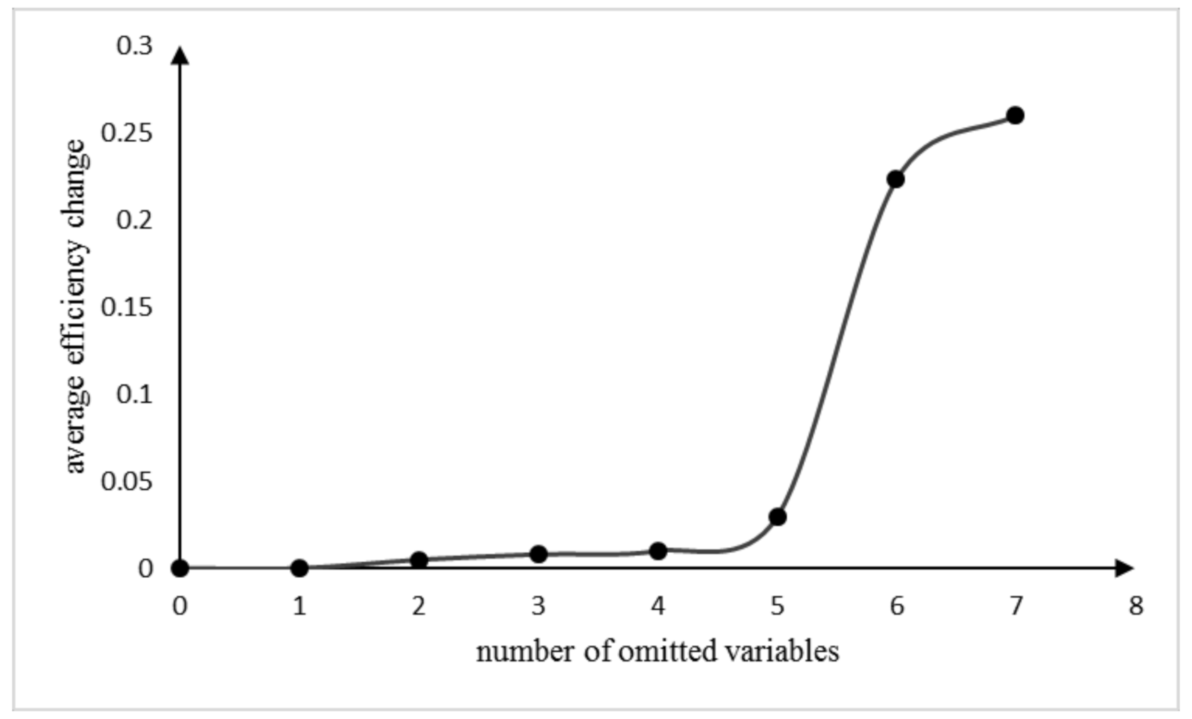
shows the efficiency scores of each DMU. The last row in Table 10 indicates the average change in the efficiency score. At the beginning, the analysis of the ratio model containing all six ratio variables yields four efficient banks (B6, B12, B14, and B15). For Case 1, removing “Current Ratio” shows the smallest average change in the efficiency scores (2.62E−10). When it is omitted from the model, the same four banks remain efficient. For Case 2 with four ratio variables, “Current Ratio” and “Profit Margin” are selected to be dropped with an average change in efficiency score of 0.008 resulting in the same efficient banks.

For Case 3, the ratio variables of “Return on Total Assets”, “Price Earning Ratio” and “Dividend Pay-Out” are kept and the average change in the efficiency score is 0.0223. For Case 4 with two ratio variables, “Return on Total Assets” and “Price Earning Ratio” are kept and the average change in the efficiency score is 0.0457. For Case 5 with only one variable (“Dividend Pay-Out”) kept, a fairly large average change in the efficiency score of 0.094 occurs. The efficiency scores for some DMUs (e.g., B6) are reduced by as much as 59%. In this case, there is only one efficient bank, i.e., B15. When the GSM algorithm is taken to its conclusion, there will always be one ratio variable identified as the most important for the efficiency score. In this US banks analysis, the key variable that has been identified for these banks is “Dividend Pay-Out” (the single remaining ratio). Managerially, we interpret this result as indicating that the core strategy for banks is to focus their capability of making profits, therefore gaining greater “Dividend Pay-Out”.

6. Implications

According to the illustrations and case studies presented in Section 5, the implications pertaining to the proposed method can be deduced. Effective decision-making approaches are fundamentally based on the ability to precisely identify a set of factors or criteria that have the greatest effect on performance. Knowledge of these factors is needed by decision-makers in taking appropriate strategy to improve their performance. This study sheds light on how the suggested methodology, which is based on the information regarding changes in efficiency ratings, is useful for evaluating efficiency, as well as offering prescriptive recommendations that managers can follow in controlling the performance of their business. This study improves the DEA method for measuring efficiency, which is a crucial notion in performance. It provides a searching method for variable selection, which includes factors having the greatest influence on the DEA findings, and the methodology is based on an optimization method.

This research provides important management insights for decision-makers to make trustworthy decisions and to utilize as recommendations to alter or symmetrize their plans and needs with effective resource allocation. According to the results of the preceding investigation, the proposed GSM model outperformed the standard DEA model in terms of performance variable selection. The GSM model examined the general guidelines of maintaining a symmetry between the number of DMUs and the number of variables. The model also specifies which variables should be used and provides alternatives for various decision-making scenarios. The method can assist decision-makers in identifying the important input and output factors that have the greatest impact on efficiency.

7. Concluding Remarks

In conclusion, the present study has proposed a GSM model to select the optimal combinations of input and output variables in DEA efficiency analysis. This method acts directly upon information regarding the change in the efficiency scores and it provides tips for DMUs as to which input or output variable has the most influence in maintaining the efficiency. Nevertheless, it is significant to note that the process of making a strategic decision is complex and can be affected by many factors (e.g., negotiation, persuasion and environment). Therefore, in future it is suggested to focus on the efficient variables selection and their impacts on ensemble selection with the issue of fuzzy and big datasets, which will help decision-makers to refine the performance estimation. In particular, investigations as to whether the required number of variables in terms of classes can be relaxed are required and the effect of using different DEA models needs further analysis.

References

1. Zhu, D. A hybrid approach for efficient ensembles. Decis. Support Syst. 2010, 48, 480–487. [Google Scholar] [CrossRef] [Green Version]
2. Zheng, Z.; Padmanabhan, B. Constructing Ensembles from Data Envelopment Analysis. INFORMS J. Comput. 2007, 19, 486–496. [Google Scholar] [CrossRef] [Green Version]
3. Provost, F.; Fawcett, T. Robust Classification for Imprecise Environments. Mach. Learn. 2001, 42, 203–231. [Google Scholar] [CrossRef]
4. Baumgartner, D.; Serpen, G. Performance of global-local hybrid ensemble versus boosting and baggin ensembles. Int. J. Mach. Learn. Cybern. 2013, 4, 301–317. [Google Scholar] [CrossRef]
5. Charnes, A.; Cooper, W.; Rhodes, E. Measuring the efficiency of decision-making units. Eur. J. Oper. Res. 1979, 3, 339. [Google Scholar] [CrossRef]
6. Cooper, W. Data Envelopment Analysis in Encyclopedia of Operations Research and Management Science; Gass, S., Fu, M., Eds.; Springer: Berlin/Heidelberg, Germany, 2013; pp. 349–358. [Google Scholar]
7. Jomthanachai, S.; Wong, W.-P.; Lim, C.-P. A Coherent Data Envelopment Analysis to Evaluate the Efficiency of Sustainable Supply Chains. IEEE Trans. Eng. Manag. 2021, PP, 1–18. [Google Scholar] [CrossRef]
8. Misiunas, N.; Oztekin, A.; Chen, Y.; Chandra, K. DEANN. A healthcare analytic methodology of data envelopment analysis and artificial neural networks for the prediction of organ recipient functional status. Omega 2016, 58, 46–54. [Google Scholar]
9. Zhu, Q.; Wu, J.; Song, M. Efficiency evaluation based on data envelopment analysis in the big data context. Comput. Oper. Res. 2018, 98, 291–300. [Google Scholar] [CrossRef]
10. Golany, B.; Roll, Y. An application procedure for DEA. Omega 1989, 17, 237–250. [Google Scholar] [CrossRef]
11. Jenkins, L.; Anderson, M. A multivariate statistical approach to reducing the number of variables in data envelopment analysis. Eur. J. Oper. Res. 2003, 147, 51–61. [Google Scholar] [CrossRef]
12. Morita, H.; Avkiran, N.K. Selecting inputs and outputs in data envelopment analysis by designing statistical experiments(Operations Research for Performance Evaluation). J. Oper. Res. Soc. Jpn. 2009, 52, 163–173. [Google Scholar] [CrossRef] [Green Version]
13. Cooper, W.W.; Seiford, L.M.; Tone, K. Data Envelopment Analysis: A Comprenhensive Text with Models, Applications, Ref-erences and DEA-Solver Software, 2nd ed.; Springer: Berlin/Heidelberg, Germany, 2007. [Google Scholar]
14. Nunamaker, T.R. Using data envelopment analysis to measure the efficiency of non-profit organizations: A critical evaluation. Manag. Decis. Econ. 1985, 6, 50–58. [Google Scholar] [CrossRef]
15. Chilingerian, J.A. Evaluating physician efficiency in hospitals: A multivariate analysis of best practices. Eur. J. Oper. Res. 1995, 80, 548–574. [Google Scholar] [CrossRef]
16. Salinas-Jimenez, J.; Smith, P. Data envelopment analysis applied to quality in primary health care. Ann. Oper. Res. 1996, 67, 141–161. [Google Scholar] [CrossRef]
17. Appa, G.; Norman, M.; Stoker, B. Data Envelopment Analysis: The Assessment of Performance. J. Oper. Res. Soc. 1992, 43, 919. [Google Scholar] [CrossRef]
18. Banker, R.D. Hypothesis tests using data envelopment analysis. J. Prod. Anal. 1996, 7, 139–159. [Google Scholar] [CrossRef]
19. Pastor, J.T.; Ruiz, J.L.; Sirvent, I. A Statistical Test for Nested Radial Dea Models. Oper. Res. 2002, 50, 728–735. [Google Scholar] [CrossRef]
20. Amirteimoori, A.; Despotis, D.K.; Kordrostami, S. Variables reduction in data envelopment analysis. Optimization 2012, 63, 735–745. [Google Scholar] [CrossRef]
21. Toloo, M.; Barat, M.; Masoumzadeh, A. Selective measures in data envelopment analysis. Ann. Oper. Res. 2015, 226, 623–642. [Google Scholar] [CrossRef]
22. Wagner, J.M.; Shimshak, D.G. Stepwise selection of variables in data envelopment analysis: Procedures and managerial per-spectives. Eur. J. Operat. Res. 2007, 180, 57–67. [Google Scholar] [CrossRef]
23. Halkos, G.E.; Salamouris, D.S. Efficiency measurement of the Greek commercial banks with the use of financial ratios: A data envelopment analysis approach. Manag. Account. Rese. 2004, 15, 201–224. [Google Scholar] [CrossRef]
24. Hofri, M. “Introduction,” in Probabilistic Analysis of Algorithms: On Computing Methodologies for Computer Algorithms Performance Evaluation; Springer: New York, NY, USA, 1987; pp. 1–10. [Google Scholar]
25. Rayward-Smith, V.J.; Cormen, T.H.; Leiserson, C.E.; Rivest, R.L. Introduction to Algorithms. J. Oper. Res. Soc. 1991, 42, 816. [Google Scholar] [CrossRef]
Figure 1. The flow chart of the GSM algorithm for case I.
Symmetry 13 01155 g001
Figure 2. The average efficiency change will increase if more variables are omitted.
Symmetry 13 01155 g002