
Symmetric Reciprocal Symbiosis Mode of China’s Digital Economy and Real Economy Based on the Logistic Model

Abstract
:1. Introduction
2. Literature Overview
2.1. The Characteristics of Digital Economy
2.2. Overview of Industrial Convergence Theory
2.3. Overview of Industrial Coevolution Theory
3. Research Methodology
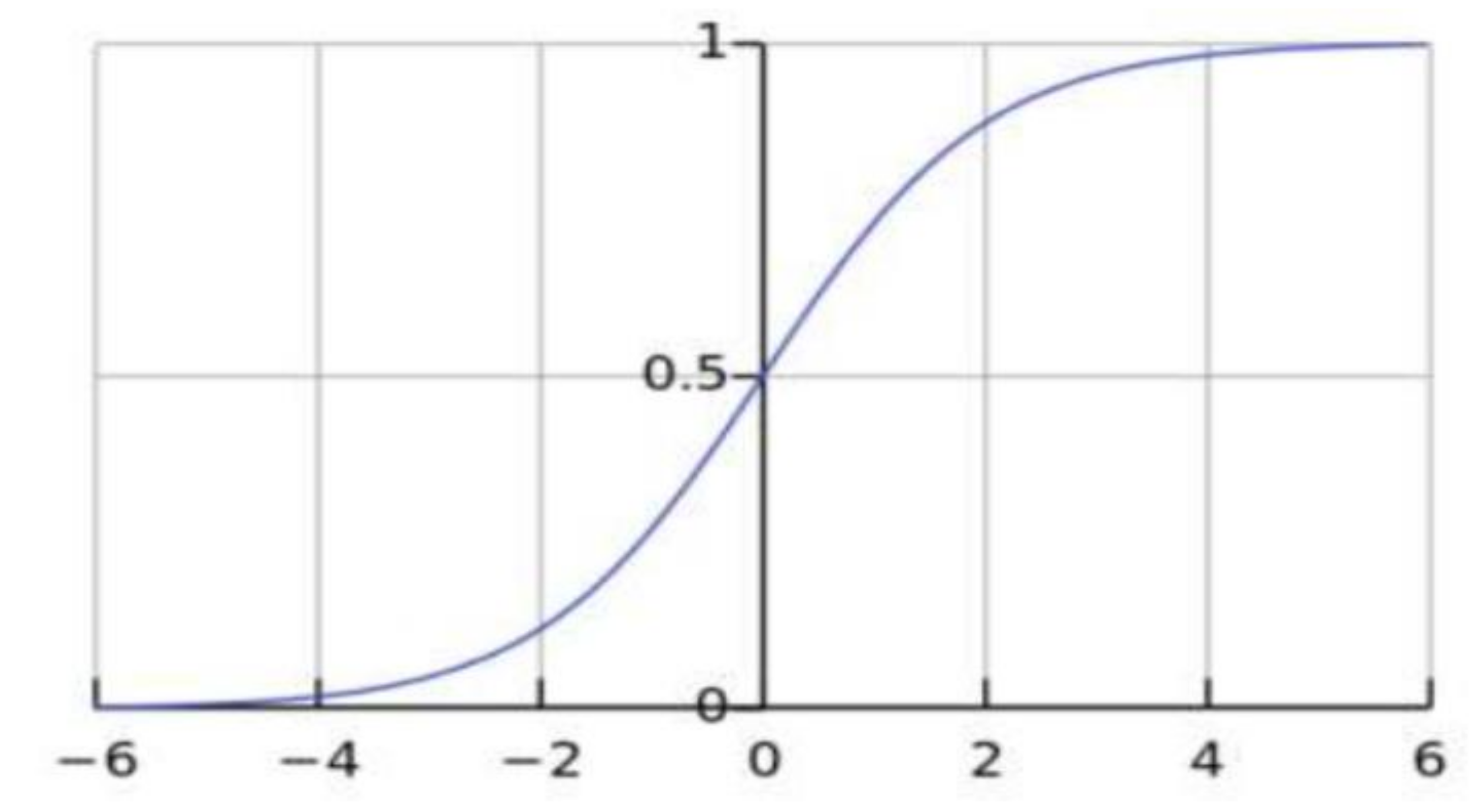
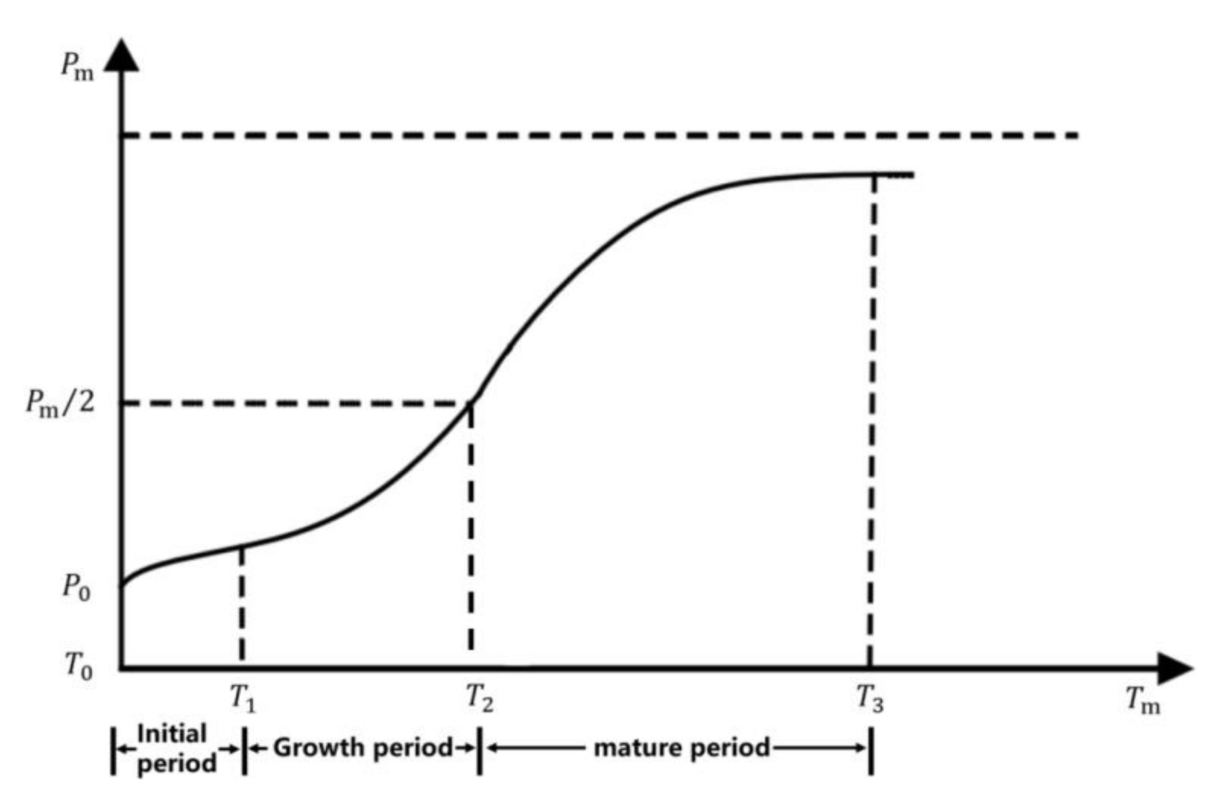
3.1. Logistic Evolution Model
3.2. Model Construction
- Independent development of the digital economy and real economy
- The interacting development of the digital economy and real economy
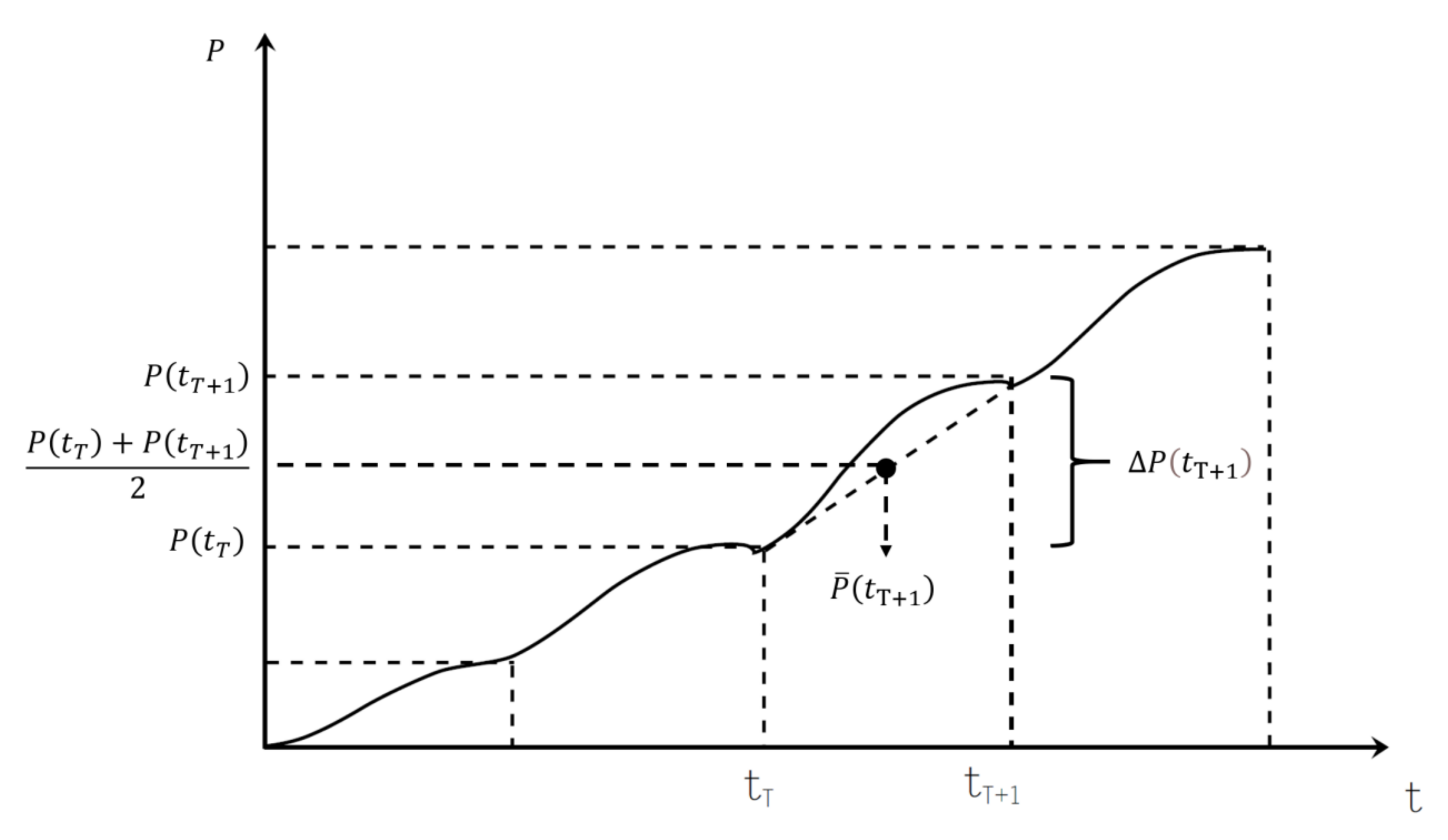
3.3. Parameter Estimation Method
- Standardizing the data
- Finding the information entropy value of each indicator
- Determining the weight of each indicator
3.4. Variable Selection and Data Source
3.4.1. Variable Selection
- (1)
- The statistics of the digital economy include C39 (computer, communication and other electronic equipment manufacturing) and I63~I65 (information transmission, software and information technology service industry).
- (2)
- The statistics of the real economy statistics include:
3.4.2. Data Sources
4. Empirical Research
4.1. Analysis of the Coevolution Model
- (1)
- The first step: Using Equations (14) to (21) to calculate the annual intrinsic growth rate and maximum environmental capacity under the independent development of the digital economy and real economy from 2005 to 2019. Since this part of the data is large and only used for subsequent calculations, the processing data is not displayed. If readers are interested, they can obtain this part of data from the authors.
- (2)
- The second step: Calculating the population growth rate () and the maximum environmental capacity of the population () under the interacting development between the digital economy and real economy from 2005 to 2019 by adopting the Equations (22) to (25). Similarly, since this part of the data is large and only used for subsequent calculations, the processing data is not displayed. If readers are interested, they can obtain this part of data from the authors.
- (3)
- The third step: The intrinsic growth rate (, ) and the maximum environmental capacity ( and ) under the independent development can be obtained through the first step. Meanwhile, the natural growth rate ( and )and the maximum environmental capacity ( and ) under the interacting development are obtained through the second step. Furthermore, the coevolution factors ( and ) of the digital economy and real economy in the four dimensions (A1, A2, B1, and B2) after incorporating the above parameters into Equation (26) can be identified.
- (4)
- The fourth step: The entropy value can be obtained after standardizing the data of A1, A2, B1, and B2 respectively. The weight of each dimension index is determined by the entropy value as illustrated in Table 3:
4.2. Simulation of the Coevolution Path of Digital Economy and Real Economy
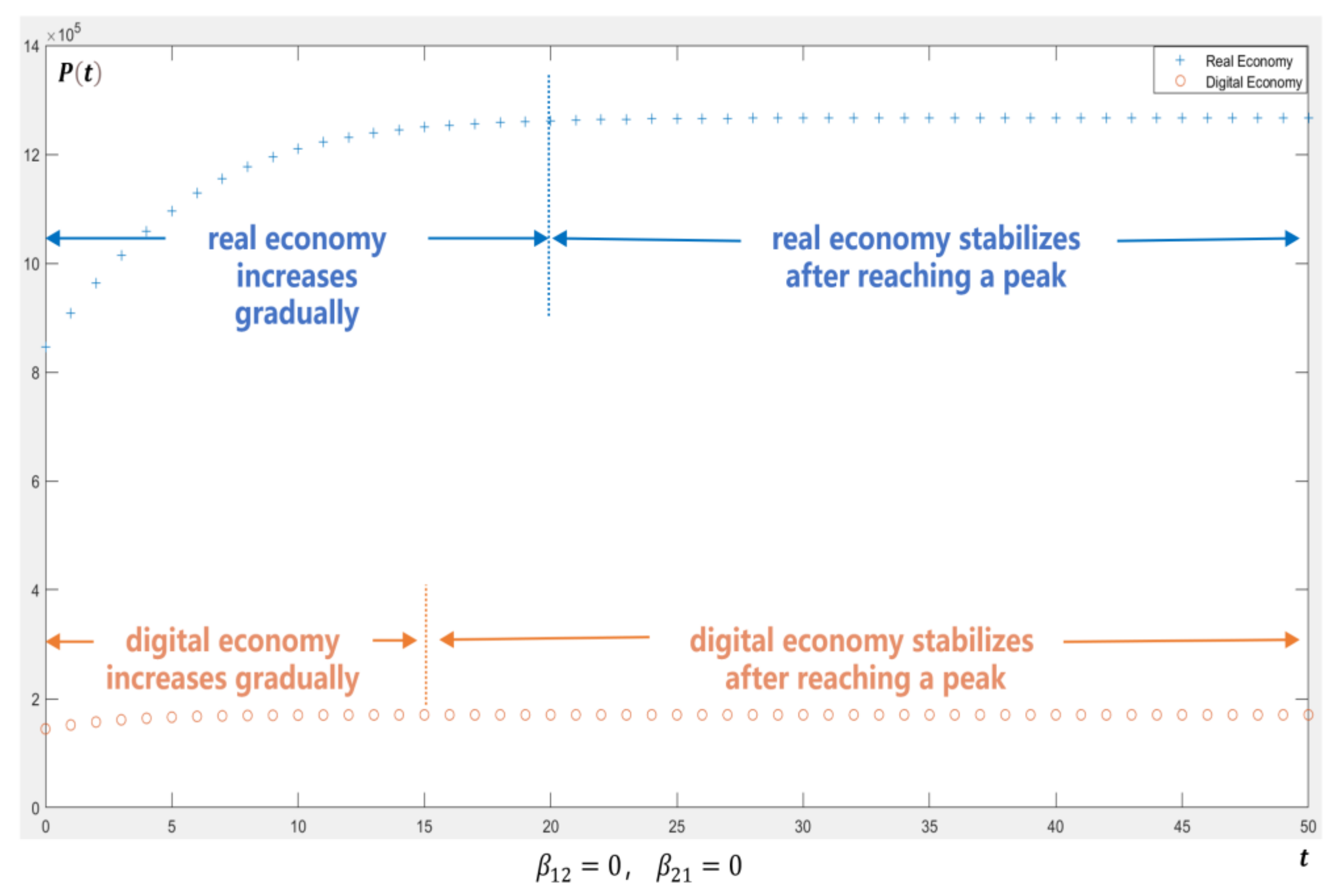
- Independent mode:
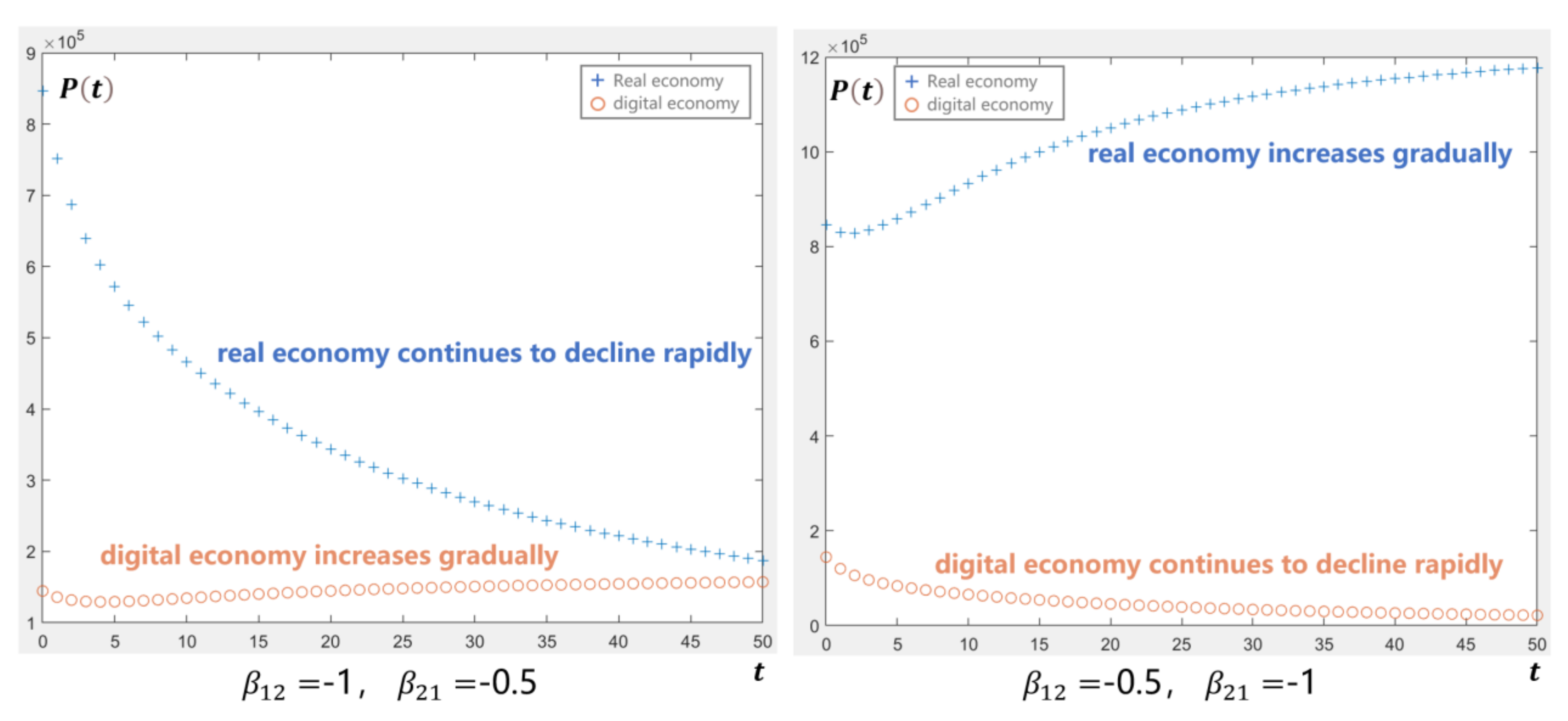
- Competition mode:
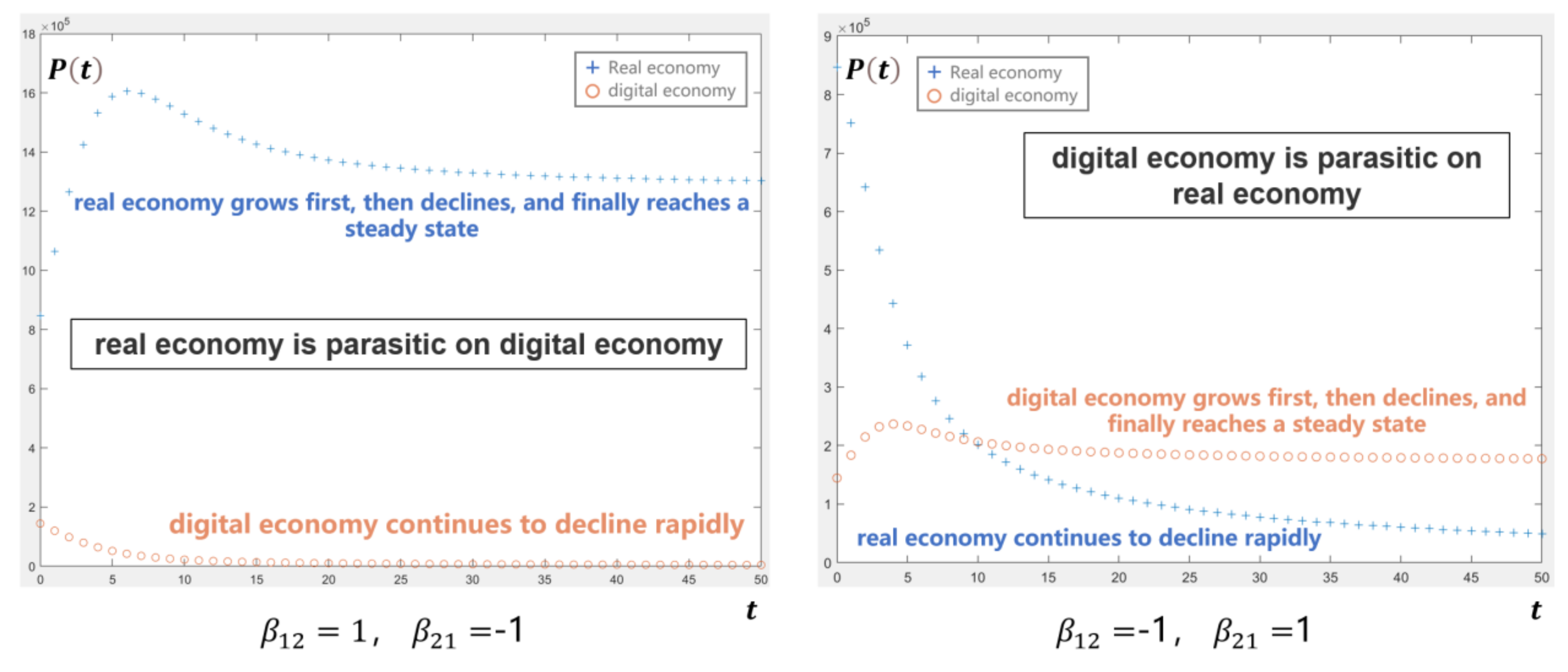
- Parasitism mode
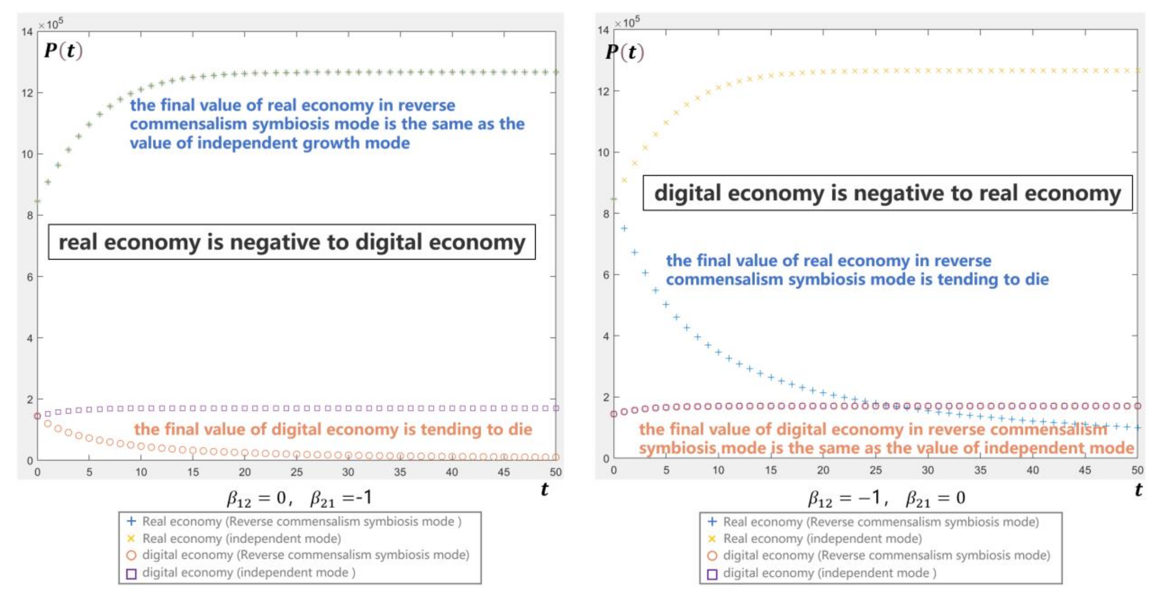
- Commensalism symbiosis/Reverse commensalism symbiosis modes
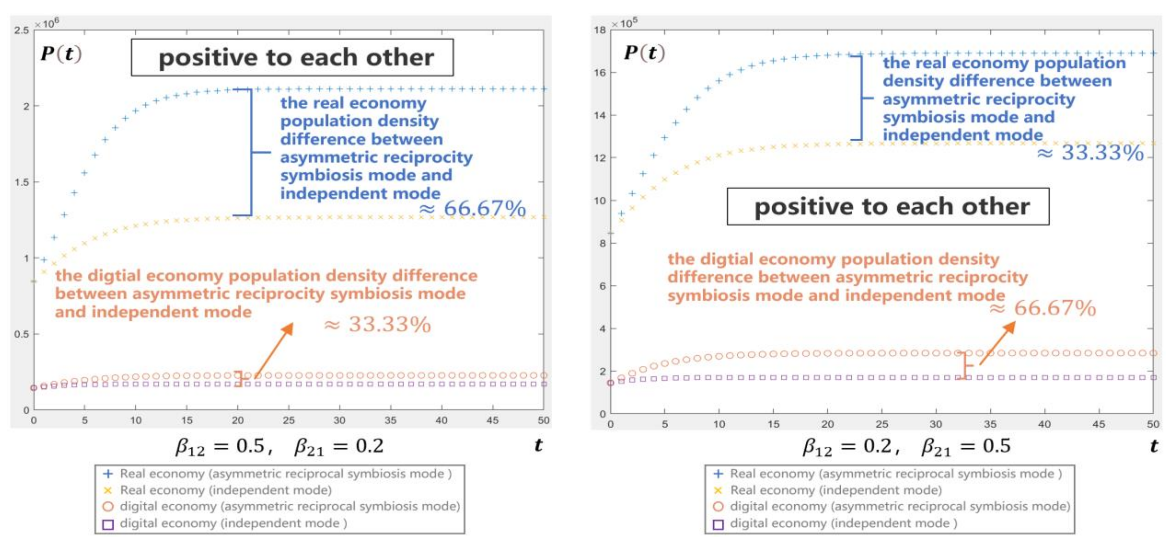
- Asymmetric reciprocal symbiosis mode
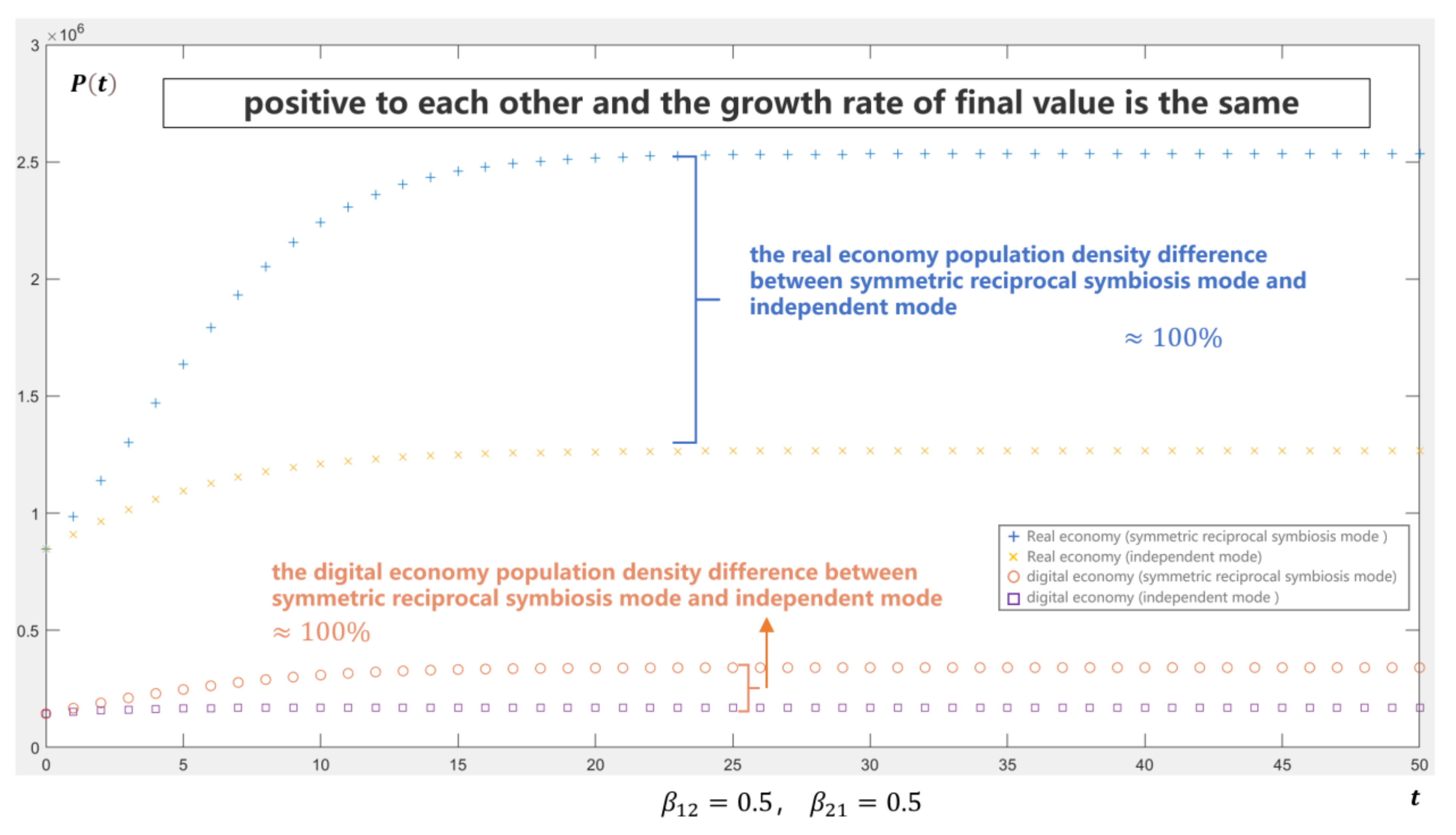
- Symmetric reciprocal symbiosis mode
5. Conclusions
- (1)
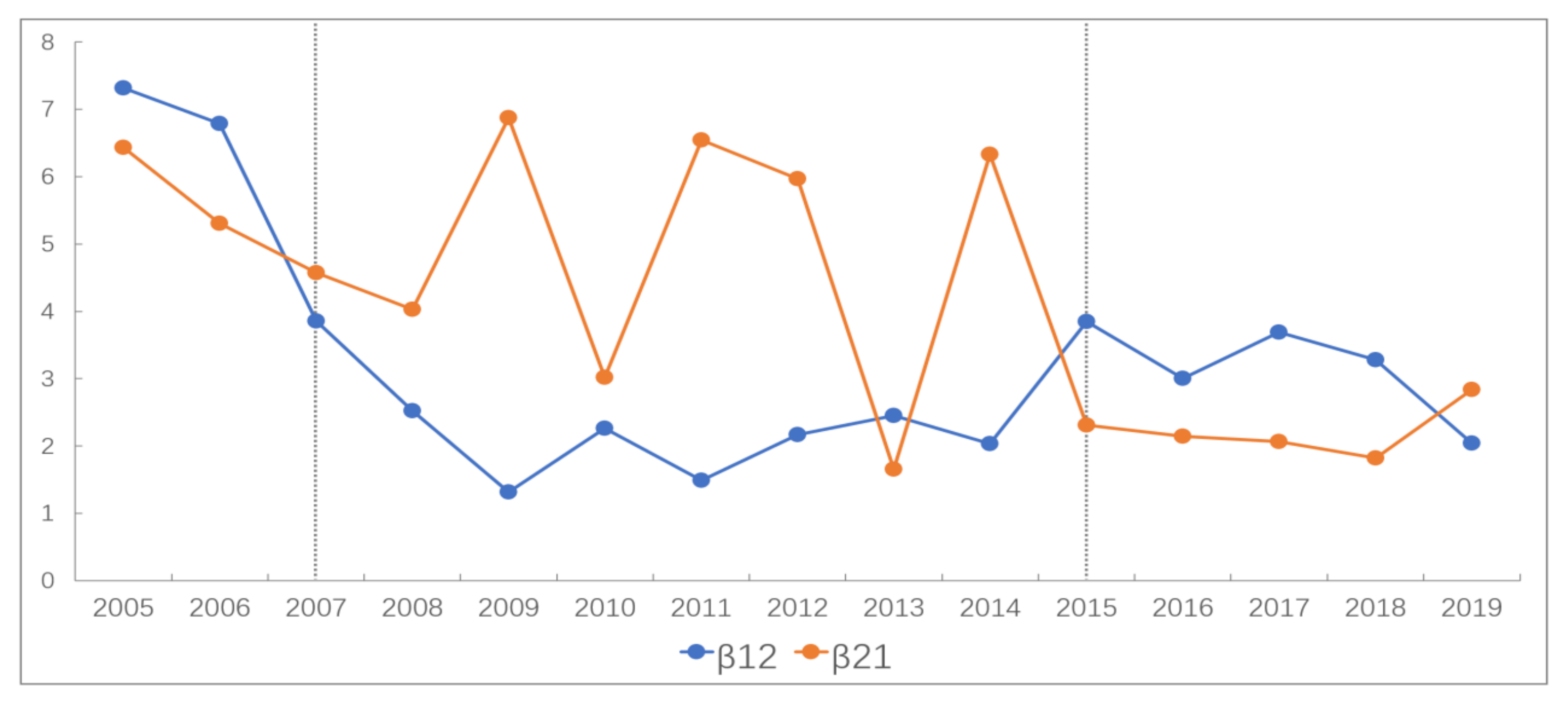
- Generally speaking, the relationship between the digital economy and the real economy during the period from 2005 to 2019 was the asymmetric reciprocal symbiosis mode. From 2005 to 2007, the real economy’s positive driving role in the digital economy was greater than the digital economy’s enabling role in the real economy when the scale and level of development of the digital economy were relatively low. From 2008 to 2015, the rapid growth of the digital economy benefited from the explosive growth of the consumer internet industry, which made much greater impacts on real economy comparing with the positive driving effect of the real economy. From 2016 to 2019, the coevolution coefficient of the digital economy and real economy continued to converge, and the real economy’s positive driving role was slightly higher than the digital economy’s enabling effect.
- (2)
- The relationship between the digital economy and primary industry was overall in the asymmetric reciprocal symbiosis mode during the period from 2005 to 2019. From 2005 to 2008, the driving effect of primary industry on the digital economy was greater than the enabling the role of digital economy. Gradually, the depth of the convergence of the digital economy and primary industry was insufficient from 2009 to 2015, therefore, the coordination coefficient showed an unstable and fluctuating state. From 2016 to 2019, the driving effect of primary industry was again higher, which indicated that the convergence needed to be in close connection with the characteristics of the primary industry to carry out the innovation and practice of digital transformation.
- (3)
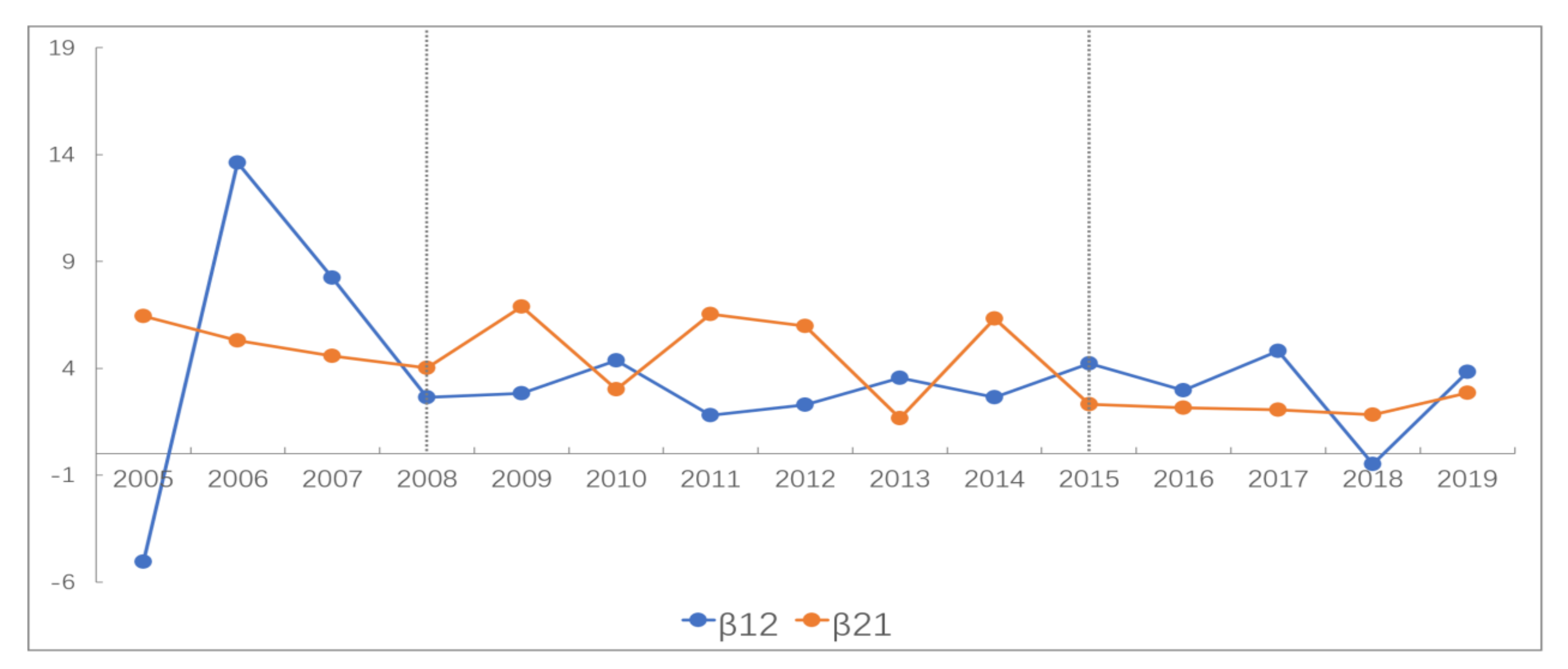
- During the period from 2005 to 2019, the overall relationship between the digital economy and secondary industry was also in the asymmetric reciprocal symbiosis mode. From 2005 to 2008, secondary industry played a stronger role in the digital economy, which effectively promoted the transition from the initial stage to the growth one. The co-evolutionary factors from 2009 to 2014 flipped back and forth while the enabling effect of the digital economy was gradually increasing. The role of secondary industry in driving the digital economy was significantly greater from 2015 to 2017; however, from 2018 to 2019, the convergence entered the “deep water” area. The technological dividends in the previous development had been fully released and digital infrastructure had become the main driving force for the coordinated development of the digital economy and secondary industry.
- (4)
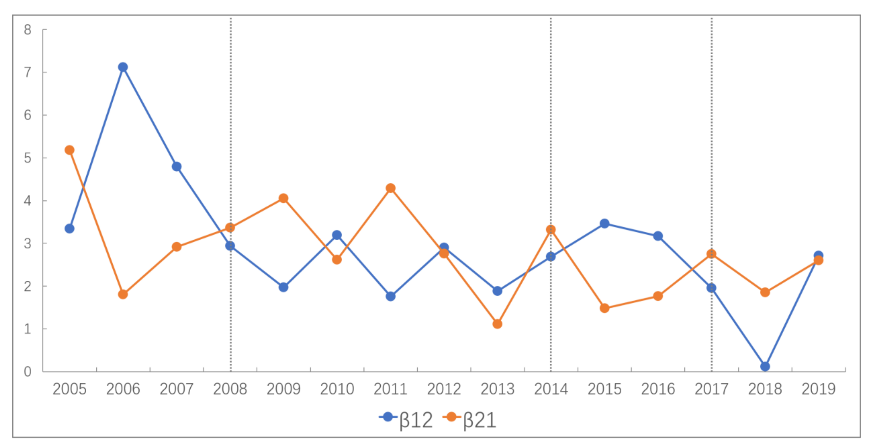
- The relationship between the digital economy and tertiary industry evolved from an asymmetric reciprocal symbiosis mode to a symmetric reciprocal symbiosis mode from 2005 to 2019. Tertiary industry made a strong driving effect on the digital economy during the period from 2005 to 2008. However, the co-evolutionary factors changed from declining growth to convergence along with the increasing influences of the digital economy from 2009 to 2014. Moreover, the convergence reached a high level, which further converged the co-evolutionary factors from 2015 to 2019. Thus, the previous mode developed into the symmetric reciprocal symbiosis mode.
- (5)
- Through simulation analysis, it could be found that the digital economy and real economy did not interfere with each other and the increasing trend was stabilizing while they were in the independent mode. Nevertheless, in the competitive mode, parasitism mode or reverse commensalism symbiosis, one of both sides would always be negatively affected by the reverse effect of the other, which would be a declining risk of population density or even extinction. In other words, the effect of coevolution was not effective. Moreover, when the two major economies were in the commensalism symbiosis mode or the asymmetric reciprocity symbiosis mode, one of the two would be affected from the positive synergy to increase the population density with better coevolution effect. While in the symmetric reciprocal symbiosis mode, the final value added would increase more than the value in the asymmetric reciprocal symbiosis mode. Consequently, the symmetric reciprocal symbiosis mode should be the best mode for realizing the convergence of China’s digital economy and real economy.
Author Contributions
Funding
Institutional Review Board Statement
Informed Consent Statement
Data Availability Statement
Conflicts of Interest
References
- Hanna, N. Mastering Digital Transformation; Emerald Publishing: Bingley, UK, 2016. [Google Scholar]
- Avi, G.; Catherine, T. Digital economics. J. Econ. Lit. 2019, 1, 3–43. [Google Scholar]
- Martin, H.R. From Industrial Economics to Digital Economics: An Introduction to the Transition; ECLAC: Mexico City, Mexico, 2001. [Google Scholar]
- Eric, B.; Nicolas, C. Internet and Digital Economics: Principles, Methods and Applications; Cambridge University Press: Cambridge, UK, 2007. [Google Scholar]
- Tong, F.; Zhang, G. The Connotation Characteristics, Unique Advantages and Path Dependence of China’s Development of Digital Economy. Science and Technology Management Research 2020, 40, 262–266. [Google Scholar]
- Yang, X. Digital Economy: Economic Logic of In-depth Transition of Traditional Economy. J. Shenzhen Univ. (Humanit. Soc. Sci.) 2017, 34, 101–104. [Google Scholar]
- OECD. OECD Digital Economy Outlook 2017; OECD Publishing: Paris, France, 2017. [Google Scholar]
- Metcalfe, B. Metcalfe’s Law: Network Becomes more Valuable as it Reaches More Users. InfoWorld 1995, 17, 53. [Google Scholar]
- Yoffie, D.B. Competing in the Age of Digital Convergence (Hardcover); Harvard Business School Press: Boston, MA, USA, 1997; p. 1. [Google Scholar]
- Uekusa, M. Mix of Communication and Information Industry. China Ind. Econ. 2001, 2, 24–27. [Google Scholar]
- Curran, C.S.; Broring, S.; Leker, J. Anticipating converging industries using publicly available data. Technol. Forecast. Soc. Chang. 2010, 77, 385–395. [Google Scholar] [CrossRef]
- Curran, C.S.; Leker, J. Patent indicators for monitoring convergence–examples from NFF and ICT. Technol. Forecast. Soc. Chang. 2011, 78, 256–273. [Google Scholar] [CrossRef]
- Yu, R.G.; Li, Y. The Impact of Industrial Convergence on the Policy of Industrial Organization. Financ. Trade Econ. 2004, 10, 18–22. [Google Scholar]
- Yu, G.R.; Li, Y. Research on technology Innovation and Industry Integration. Product. Res. 2003, 6, 175–177. [Google Scholar]
- Yu, R.G. The classification of three industries and the trend of industry integration. Rev. Econ. Res. 1997, 25, 46–47. [Google Scholar]
- Xie, K.; Xiao, J.; Zhou, X.; Wu, J. Quality of Integration of Industrialization and informatization in China: Theory and Demonstration. Zhongguo Xinxihua 2017, 4, 71–83. [Google Scholar]
- Xie, K.; Xiao, J. Integration of Industrialization and informatization: A theoretical model. J. Sun Yatsen Univ. (Soc. Sci. Ed.) 2011, 51, 210–216. [Google Scholar]
- Xiao, J.; Xie, K.; Zhou, X.; Wu, J. The Development Model of Informatization-Promoting-Industrialization. J. Sun Yatsen Univ. (Soc. Sci. Ed.) 2006, 46, 98–104. [Google Scholar]
- Nelson, R.R. The Co-evolution of Technology, Industrial Structure, and Supporting Institutions. Ind. Corp. Chang. 1994, 3, 47–63. [Google Scholar] [CrossRef]
- Murmann, J.P. Knowledge and Competitive Advantage: Knowledge and Competitive Advantage: The Coevolution of Firms, Technology, and National Institutions; Cambridge University Press: Cambridge, UK, 2003. [Google Scholar]
- Huang, K. Comments on the Theory of Coevolution. J. China Univ. Geosci. (Soc. Sci. Ed.) 2008, 4, 97–101. [Google Scholar]
- Li, D.; Xiang, B. Review on the co evolution theory of organization and environment. Foreign Econ. Manag. 2007, 29, 9–17. [Google Scholar]
- Zhang, Q. An Empirical Study on the Co-Evolution of China’us Manufacturing Industry and Productive Service Industry; LiaoNing University: Shenyang, China, 2018. [Google Scholar]
- Verhulst, P.F. Recherches mathématiques sur la loi d’accroissement de la population. Nouveaux Mémoires de l’Académie Royale des Sciences et Belles-Lettres de Bruxelles 1845, 1, 1–42. [Google Scholar]
- Michael, G.; Steven, K. Time Paths in the Diffusion of Product Innovations. Econ. J. 1982, 92, 630–653. [Google Scholar]
- Pang, B.H. Research About Symbiotic Evolutionary Model of Producer Services and Manufacturing Industry in China. Chin. J. Manag. Sci. 2012, 20, 176–183. [Google Scholar]
- Tang, R.Q.; Xu, X.L.; He, Z.L. A Model and Empirical Study of the Symbiotic Develop-ment between the Producer-service Industry and the Manufacturing Industry. Nankai Bus. Rev. 2009, 12, 20–26. [Google Scholar]
- Olsson, D.M.; Nelson, L.S. The Nelder-Mead simplex procedure for function minimization. Technometrics 1975, 17, 45–51. [Google Scholar] [CrossRef]
- Ahn, B. Compatible weighting method with rank order centroid: Maximum entropy ordered weighted averaging approach. Eur. J. Oper. Res. 2011, 212, 552–559. [Google Scholar] [CrossRef]
- Citil, H.G. Important Notes for a Fuzzy Boundary Value Problem. Appl. Math. Nonlinear Sci. 2019, 4, 305–314. [Google Scholar] [CrossRef] [Green Version]
- Jefferson, G.H.; Rawski, T.G.; Zhang, Y. Productivity growth and convergence across China’s industrial economy. J. Chin. Econ. Bus. Stud. 2008, 6, 121–140. [Google Scholar] [CrossRef]
- Kwon, O.; An, Y.; Kim, M.; Lee, C. Anticipating technology-driven industry convergence: Evidence from large-scale patent analysis. Technol. Anal. Strateg. Manag. 2020, 32, 363–378. [Google Scholar] [CrossRef]
- Kim, N.; Lee, H.; Kim, W.; Lee, H.; Suh, J.H. Dynamic patterns of industry convergence: Evidence from a large amount of unstructured data. Res. Policy 2015, 44, 1734–1748. [Google Scholar] [CrossRef]
- Yu, S. Research on the Relationship between Virtual Economy and Real Economy Development in China. J. Phys. Conf. Ser. 2019, 1237, 2. [Google Scholar]
- Taddeo, R.; Simboli, A.; Morgante, A.; Erkman, S. The development of industrial symbiosis in existing contexts. Experiences from three Italian clusters. Ecol. Econ. 2017, 139, 55–67. [Google Scholar] [CrossRef]
- Lawal, M.; Alwi, S.R.W.; Manan, Z.A.; Ho, W.S. Industrial symbiosis TOOLS—A review. J. Clean. Prod. 2020, 280, 1–20. [Google Scholar]
- Li, Y.Y. Industry Convergence, Technology Progress and the Growth of Hi-Tech Industry. J. Converg. Inf. Technol. 2013, 8, 946–953. [Google Scholar]
- National Bureau of Statistics of China, Web of National Bureau of Statistics of China. National Bureau of Statistics of China. Available online: http://www.stats.gov.cn/tjsj/tjbz/ (accessed on 15 October 2020).
- G20 Research Group. G20 digital economy development and cooperation initiative. G20 Res. Group Univ. Tor. 2016, 1, 1–9. [Google Scholar]
- Kevin, B.; Curtis, D.; Jolliff, W.; Nicholson, J.R.; Omohundro, R. Defining and measuring the digital economy. US Dep. Commer. Bur. Econ. Anal. Wash. DC 2018, 15, 1–25. [Google Scholar]
- Zhang, D. A Brief Analysis of the Status Quo of Russian Digital Economy. Russ. Stud. 2018, 2, 130–158. [Google Scholar]
- National Bureau of Statistics of China. Web of National Bureau of Statistics of China. Available online: http://www.stats.gov.cn/tjsj/ndsj/ (accessed on 16 October 2020).
- Ministry of Industry and Information Technology of the People’s Republic of China. Annual Statistical Report on Software and Information Technology Services Industry of China. 2019. Available online: https://www.miit.gov.cn/jgsj/xxjsfzs/xyyx/art/2020/art_7431516acb7944b38db842281c7eebba.html (accessed on 16 October 2020).


| Number | Value | Mode | Characteristics |
|---|---|---|---|
| 1 | Independent | Two economies develop independently and there is no symbiotic relationship. | |
| 2 | , | Competition | Digital economy and real economy compete for the resources. |
| 3 | , | Parasitism | One side achieves growth while restraining the other side’s growth |
| 4 | , | Commensalism symbiosis | One side’s growth drives the other side’s growth, yet other side’s growth does not promote itself. |
| 5 | , | Reverse commensalism symbiosis | One side’s growth restricts the growth of the other side while the growth of the other side does not promote itself. |
| 6 | , | Asymmetric reciprocal symbiosis | When one side achieves growth to drive the growth of the other side, the growth of the other side will drive the growth of itself, but the driving effect is asymmetric. |
| 7 | , | Symmetric reciprocal symbiosis | When one side’s growth to drive the growth of the other side, the growth of the other side will promote its own growth and the driving effects are symmetric. |
| Indicators | Index | Dimension | Definitions | Unit |
|---|---|---|---|---|
| A1 | Economic benefits | Value Added | Value added of industries | Billion Yuan |
| A2 | Fixed asset investment | Total investment in fixed assets | Billion Yuan | |
| B1 | Social benefits | Number of employees | Total employed persons | thousand people |
| B2 | Number of market players | Number of enterprises or legal persons | person |
| Indicators | A1 | A2 | B1 | B2 |
|---|---|---|---|---|
| Real economy | 0.2369 | 0.2550 | 0.1589 | 0.3492 |
| Primary industry | 0.1655 | 0.2813 | 0.1897 | 0.3636 |
| Secondary industry | 0.2598 | 0.2884 | 0.1267 | 0.3251 |
| Tertiary Industry | 0.2244 | 0.2306 | 0.2334 | 0.3115 |
| Digital economy | 0.1822 | 0.2960 | 0.1383 | 0.3835 |
| Year | β12(t) | β21(t) |
|---|---|---|
| 2005 | 7.3153 | 6.4296 |
| 2006 | 6.7875 | 5.3037 |
| 2007 | 3.8526 | 4.5708 |
| 2008 | 2.5247 | 4.0273 |
| 2009 | 1.3168 | 6.8785 |
| 2010 | 2.2655 | 3.0160 |
| 2011 | 1.4927 | 6.5439 |
| 2012 | 2.1661 | 5.9663 |
| 2013 | 2.4509 | 1.6565 |
| 2014 | 2.0316 | 6.3297 |
| 2015 | 3.8475 | 2.3099 |
| 2016 | 3.0061 | 2.1403 |
| 2017 | 3.6873 | 2.0617 |
| 2018 | 3.2825 | 1.8208 |
| 2019 | 2.0396 | 2.8411 |
| Year | β12(t) | β21(t) |
|---|---|---|
| 2005 | −5.0619 | 6.4296 |
| 2006 | 13.6245 | 5.3037 |
| 2007 | 8.2317 | 4.5708 |
| 2008 | 2.6345 | 4.0273 |
| 2009 | 2.8237 | 6.8785 |
| 2010 | 4.3606 | 3.0160 |
| 2011 | 1.8047 | 6.5439 |
| 2012 | 2.2928 | 5.9663 |
| 2013 | 3.5478 | 1.6565 |
| 2014 | 2.6307 | 6.3297 |
| 2015 | 4.2342 | 2.3099 |
| 2016 | 2.9559 | 2.1403 |
| 2017 | 4.8095 | 2.0617 |
| 2018 | −0.4861 | 1.8208 |
| 2019 | 3.8364 | 2.8411 |
| Year | β12(t) | β21(t) |
|---|---|---|
| 2005 | 3.3439 | 5.1772 |
| 2006 | 7.1164 | 1.8030 |
| 2007 | 4.7943 | 2.9180 |
| 2008 | 2.9369 | 3.3632 |
| 2009 | 1.9666 | 4.0554 |
| 2010 | 3.1895 | 2.6195 |
| 2011 | 1.7536 | 4.2862 |
| 2012 | 2.9015 | 2.7613 |
| 2013 | 1.8799 | 1.1121 |
| 2014 | 2.6862 | 3.3220 |
| 2015 | 3.4618 | 1.4820 |
| 2016 | 3.1717 | 1.7669 |
| 2017 | 1.9552 | 2.7489 |
| 2018 | 0.1203 | 1.8556 |
| 2019 | 2.7098 | 2.6012 |
| Year | β12(t) | β21(t) |
|---|---|---|
| 2005 | 6.3600 | 4.5295 |
| 2006 | 7.2471 | 2.0639 |
| 2007 | 5.4725 | 2.5091 |
| 2008 | 2.8159 | 3.1947 |
| 2009 | 1.4688 | 7.1145 |
| 2010 | 3.0172 | 3.0136 |
| 2011 | 2.1114 | 3.7690 |
| 2012 | 2.4176 | 3.1565 |
| 2013 | 1.7159 | 2.8944 |
| 2014 | 1.9620 | 4.6184 |
| 2015 | 3.2341 | 2.5901 |
| 2016 | 2.6249 | 2.4504 |
| 2017 | 3.1632 | 2.5668 |
| 2018 | 2.2756 | 2.0769 |
| 2019 | 2.3962 | 2.6412 |
Publisher’s Note: MDPI stays neutral with regard to jurisdictional claims in published maps and institutional affiliations. |
© 2021 by the authors. Licensee MDPI, Basel, Switzerland. This article is an open access article distributed under the terms and conditions of the Creative Commons Attribution (CC BY) license (https://creativecommons.org/licenses/by/4.0/).
Share and Cite
Xu, G.; Lu, T.; Liu, Y. Symmetric Reciprocal Symbiosis Mode of China’s Digital Economy and Real Economy Based on the Logistic Model. Symmetry 2021, 13, 1136. https://doi.org/10.3390/sym13071136
Xu G, Lu T, Liu Y. Symmetric Reciprocal Symbiosis Mode of China’s Digital Economy and Real Economy Based on the Logistic Model. Symmetry. 2021; 13(7):1136. https://doi.org/10.3390/sym13071136
Chicago/Turabian StyleXu, Guoteng, Tingjie Lu, and Yiman Liu. 2021. "Symmetric Reciprocal Symbiosis Mode of China’s Digital Economy and Real Economy Based on the Logistic Model" Symmetry 13, no. 7: 1136. https://doi.org/10.3390/sym13071136
APA StyleXu, G., Lu, T., & Liu, Y. (2021). Symmetric Reciprocal Symbiosis Mode of China’s Digital Economy and Real Economy Based on the Logistic Model. Symmetry, 13(7), 1136. https://doi.org/10.3390/sym13071136