Abstract
Unidirectional unsteady flows of the incompressible Burgers’ fluids between two infinite horizontal parallel plates are analytically studied when the magnetic and porous effects are taken into consideration. The fluid motion is induced by the two plates, which move in their planes with time-dependent velocities. Exact general expressions are established both for the dimensionless velocity and shear stress fields as well as the corresponding Darcy’s resistance in the channel using the Laplace transform. If both plates move with equal velocities in the same direction, the fluid motion becomes symmetric with respect to the mid-plane between them. Otherwise, its motion is non-symmetric. To bring to light the behavior of the fluid, the dimensionless velocity profiles versus the spatial variable as well as its time evolution are presented both for the symmetric and asymmetric case. Finally, for comparison, similar graphical representations are presented together for the velocities of the incompressible Oldroyd-B and Burgers’ fluids. For large values of the time t, as expected, the behavior of the two different fluids is almost identical. The Darcy’s resistance against y is also graphically represented for the symmetric flow at different values of the time t. The influence of the magnetic field on the fluid motion is graphically revealed and discussed.
1. Introduction
Earlier, Burgers [1] developed a one-dimensional linear model whose constitutive equation is given by the relation
where is the stress, is the one-dimensional strain and and are the material constants. This model was used to characterize the behavior of different viscoelastic materials such as soil, asphalt and food products such as cheese [2,3]. Lee and Markwick [4] as well as Saal and Labout [5] have shown that the mechanical behavior of asphalt can be approximated well enough by the Burgers’ model. It has also been used in determining the transient creep properties of the Earth’s mantle [6,7] and for the study of high-temperature viscoelasticity of fine-grained polycrystalline olivine [8].
Unfortunately, the constitutive formula in Equation (1) does not satisfy the objectivity principle. More exactly, neither the linearized strain nor its material time derivative is frame-indifferent. A nonlinear three-dimensional generalization of Equation (1), namely
which is frame-indifferent, was proposed by Krishan and Rajagopal [9], who used a thermodynamic framework developed by Rajagopal and Srinivasa [10] for modeling rate-type viscoelastic fluids. In the above relations, T is the Cauchy stress, is the undetermined spherical stress due to the constraint of incompressibility, S is the constitutively determined extra stress tensor, L is the gradient of the velocity field , is the fluid viscosity, and are material constants (material moduli) and the upper convected derivative is defined by
An exact solution for the velocity field corresponding to the steady motion of such a fluid in an orthogonal rheometer was obtained by Ravindran et al. [11]. Other exact solutions, albeit for unsteady motions of the incompressible Burgers’ fluids between two parallel walls perpendicular to a moving plate or over an infinite plate, were established by Khan et al. [12] and Safia et al. [13], respectively. If or in Equation (2)2, the corresponding constitutive formula in Equation (2) characterizes the incompressible Oldroyd-B, Maxwell and Newtonian fluids, respectively. In some particular cases, like the motions to be considered here, the governing equations for the Burgers’ fluids resemble those of second grade fluids. Consequently, it is expected for the present solutions to be easily particularized to give similar solutions corresponding to the above-mentioned fluids.
Magnetohydrodynamic (MHD) flows between parallel plates have been considerably investigated due to their extensive applications in science and engineering. Exact solutions for such motions of the incompressible Newtonian fluids can be found, for instance, in the book of Schlichting [14] and the review works of Wang [15,16]. The unsteady generalized Couette flow of the same fluids was studied by Erdogan [17]. The first exact solutions for the velocity field corresponding to the motions of non-Newtonian fluids (more exactly, second grade fluids) seem to be those of Rajagopal [18] and Siddiqui et al. [19]. An interesting mixed initial boundary value problem for Kelvin–Voigt fluids was studied by Baranovskii [20]. Recently, Fetecau et al. [21,22] determined exact solutions for the velocity and non-trivial shear stress fields, corresponding to the motions of the incompressible Maxwell fluids between infinite horizontal parallel plates embedded in a porous medium. To the best of our knowledge, such solutions for motions of Burgers’ fluids are lacking in the existing literature.
The purpose of this work is to provide exact solutions for some unsteady MHD flows of incompressible Burgers’ fluids through a porous medium between infinite horizontal parallel plates. The fluid motion is generated by plates which move in their planes with arbitrary time-dependent velocities. Analytical expressions are determined for the dimensionless velocity and shear stress fields as well as the corresponding Darcy’s resistance by means of Laplace transforms. They satisfy all imposed initial and boundary conditions and can be easily reduced to the similar solutions corresponding to Oldroyd-B and second grade fluids. Finally, the velocity profiles versus the spatial variable and its time variation are graphically depicted and discussed. A comparison with Oldroyd-B fluids, as well as the variation of the Darcy’s resistance in the channel, is also included.
2. Statement of the Problem and Governing Equations
Let us consider an incompressible electrically conducting Burgers’ fluid at rest in a porous medium between two infinite horizontal parallel plates at the distance d apart. A magnetic field of the uniform strength acts perpendicular to the plates. The induced magnetic field can be neglected if the magnetic Reynolds number is considered to be small enough. At the moment , both plates begin to move in their planes in the same direction with the time-dependent velocities and , where U is a constant velocity, the functions and are two derivable times and the following is true:
The motion of incompressible Newtonian fluids between two infinite horizontal parallel plates, which at the moment began to move in their planes with the same constant velocity U, was studied by Erdogan [17]. Owing to the shear, the fluid begins to move and, since the plates are boundless, all physical entities characterizing the fluid motion are functions of y and t only in a suitable Cartesian x, y and z coordinate system whose y axis is perpendicular to the plates.
Following Khan et al. [23], we are looking for a velocity field of the following form:
where i is the unit vector along the x direction of the coordinate system. If the fluid and the whole system are at rest at the moment , we assume that
By introducing the velocity field from Equation (5) into Equation (2)2 and keeping in mind the initial conditions from Equation (6), it is not difficult to prove that the components and of the extra stress tensor S are zero (see for instance Fetecau et al. [24]), while the non-trivial shear stress has to satisfy the following differential equation:
The continuity equation is clearly satisfied, while the balance of the linear momentum, in the absence of a pressure gradient in the flow direction, reduces to the following partial differential equation [23]:
where is the constant density of the fluid, is its electrical conductivity and the Darcy’s resistance has to satisfy the next differential equation [23, Equation (8)]:
where the constants k and represent the porous medium permeability and its porosity, respectively.
By eliminating between Equations (7) and (8), and bearing in mind Equation (9) for , the following partial differential equation for the dimensional velocity field is obtained:
In the above relation, is the kinematic viscosity of the fluid. The corresponding initial and boundary conditions are (see also Equation (6) for the velocity field)
By using the next non-dimensional variables and functions
in the governing expression in Equation (10) and dropping the star notation, the following initial and boundary value problem results in the non-dimensional velocity field :
In order to determine the dimensionless frictional force per unit area exerted by the fluid on the stationary plate, the non-trivial shear stress , for instance, has to be determined. To do that, the following differential equation with the initial conditions
has to be solved. In the above relation, is the Reynolds number, and the dimensionless constants , M and K are defined by the following equalities:
The non-dimensional form of Equation (9) is given by the following equality function:
In addition, the appropriate initial conditions for the dimensionless Darcy’s resistance are
3. Solution of the Problem
In the following, we shall solve the initial and boundary value problems from Equations (14–16) and the ordinary differential Equations (17) and (20) with the corresponding initial conditions by using the Laplace transform technique.
3.1. Closed Form Expression for the Velocity Field
By applying the Laplace transform to the equality in Equation (14) and bearing in mind the initial and boundary conditions in Equations (15) and (16), one obtains for the Laplace transform of the following boundary value problem:
In the above equation, the function is defined by the following relation:
In addition, the constants and are given by the following equalities:
The solution of the boundary value problem in Equation (22) is given by the relation
In order to determine the inverse Laplace transform of the right member of Equation (25), we rewrite in the following equivalent but suitable form:
where and
As the functions and satisfy the conditions of Equation (4), the result is that the inverse Laplace transforms and of and , respectively, are given by the following relations:
where the star notation “” means the convolution product of the two functions.
To determine the inverse Laplace transforms and of and , respectively, let us introduce the following auxiliary function:
whose inverse Laplace transform (see Equation (A1) from Appendix A) is as follows:
Since and , the result is that [25]
where the function (see Equations (A2) and (A3) from Appendix A) is given by the following expression:
This is the inverse Laplace transform of . In the above relation, is the standard Bessel function of the first kind of zero order and the function is defined in Appendix A. Of course, knowing the functions and , the result is that the non-dimensional velocity field is given by the following relation (see the equality in Equation (26)):
3.2. Determination of the Non-Trivial Shear Stress
Once the velocity field is known, the dimensionless non-null shear stress can be determined using the ordinary differential Equation (17) with the initial conditions from Equation (18). Consequently, by applying the Laplace transform to Equation (17) and bearing in mind the conditions in Equation (18), the result is that the Laplace transform of is given by the next equality:
where
and where . Based on the equalities in Equation (A4) from Appendix A, it is not difficult to show that the inverse Laplace transform of has the following simple form:
From Equation (26), the result is the following:
Let us now introduce a new auxiliary function, specifically
whose inverse Laplace transform is (see Equation (A1)2)
Since and , the result is that the inverse Laplace transforms and of and , respectively, are given by the following relations (see, for instance, [25]):
where the function is given by Equation (33). Consequently, the derivative of with respect to y is given by the following relation:
Additionally, the dimensionless shear stress has the following expression (see Equation (35)):
3.3. Closed Form Expression for the Dimensionless Darcy’s Resistance
By applying the Laplace transform to Equation (20) and taking into account the initial conditions of Equation (21), the result is that the inverse Laplace transform of is given by the following relation:
Consequently, the non-dimensional Darcy’s resistance in the channel is given by the following relation:
4. Some Numerical Results and Discussion
General expressions have been previously determined for the dimensionless velocity, shear stress and Darcy’s resistance, corresponding to the unsteady MHD flow of the incompressible Burgers’ fluids between two infinite horizontal parallel plates embedded in a porous medium. The main purpose of this section is to apply the obtained results to two specific cases, namely when , and with corresponding to non-symmetric and symmetric flows, respectively, with regard to the median plane between plates. In order to obtain the numerical values and the corresponding graphical representations of the non-dimensional velocity and the Darcy’s resistance given by the equalities in Equations (34) and (46), respectively, Mathcad 15 software was used to generate Figure 1, Figure 2, Figure 3, Figure 4, Figure 5, Figure 6, Figure 7, Figure 8 and Figure 9.
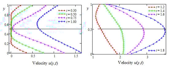
Figure 1.
The velocity profiles versus the spatial coordinate y for the non-symmetric flow.
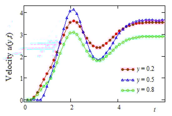
Figure 2.
The time evolution of the fluid velocity for three channel positions (non-symmetric case).
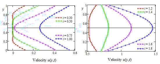
Figure 3.
The velocity profiles versus the spatial coordinate y for the symmetric flow.
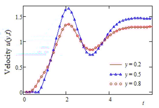
Figure 4.
The time evolution of the fluid velocity for three channel positions (symmetric case).
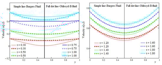
Figure 5.
The velocity profiles of the Oldroyd-B and Burgers’ fluids versus the spatial coordinate y for the symmetric flow.
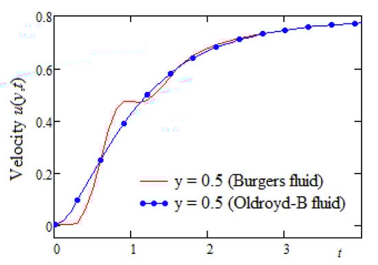
Figure 6.
Time evolution of the velocity of the Oldroyd-B fluid and Burgers’ fluid in the middle of the channel (symmetric flow).
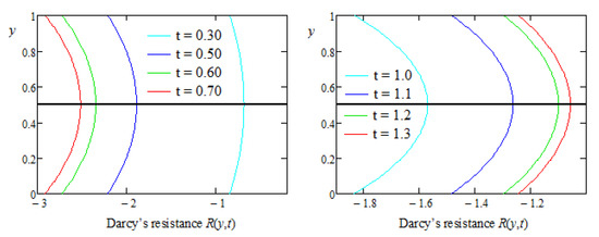
Figure 7.
Darcy’s resistance versus y for the symmetric flow.
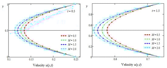
Figure 8.
The velocity profiles versus the spatial coordinate y for the symmetric flow at different values of the parameter M.
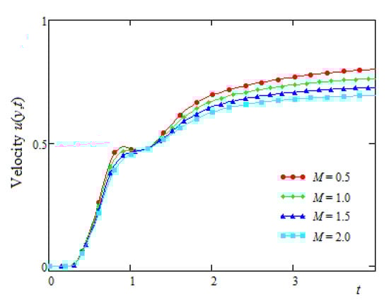
Figure 9.
Time evolution of the fluid velocity at the middle of the channel.
In Figure 1, the profiles of the non-symmetric velocity versus y at several values of the time t are presented. The velocities of the two walls of the channel slightly increased from zero to constant velocities of three and two at high values of the time t. Their movement generated the fluid’s motion and the velocity profiles change in space and time. At small values of time t, the fluid moved slower in the central area of the channel, but the opposite behavior appeared later. In addition, the curves representing the fluid velocity were asymmetric with respect to the symmetry plane of the channel. Furthermore, the fluid located in the lower semi-channel moved faster than the fluid from the upper semi-channel. Of course, this behavior was due to the fact that the speed of the lower plate was higher than the velocity of the upper one.
The time evolution of the fluid velocity at the middle of the channel (y = 0.5) and in two symmetric positions with regard to the symmetry plane of the channel, namely where and , is depicted in Figure 2. The non-symmetric aspect of the fluid velocity is clearly seen from the respective diagrams. It can also be observed that for large values of time t, the fluid velocity tended to be hold at constant asymptotic values because the walls’ velocities approached or .
Figure 3 and Figure 4 were sketched for the flow of the fluid induced by the channel’s walls, which moved in their planes with equal velocities in the same direction. As expected, in this case, the velocity profiles were symmetric with respect to the median plane of the channel. Like in Figure 1, as was to be expected, the fluid velocity increased over time. The symmetry property of the flow in this case is also highlighted in Figure 4, which clearly shows that the velocity’s diagrams corresponding to the symmetric positions are identical. In all these figures, we used the same numerical values for the dimensionless parameters, namely and For comparison, the velocities’ profiles corresponding to the Oldroyd-B () and Burgers’ fluids against y and their time evolutions at the middle of the channel are presented together in Figure 5 and Figure 6. The values of the non-dimensional material coefficients which were used here were and for the Oldroyd-B and Burgers’ fluids, respectively. At small values of time t, as is apparent from the results from the graphical representations, the Burgers’ fluid flowed slower than the Oldroyd-B fluid, but this behavior changed many times later. Figure 6 clearly shows that, as expected, for large values of time t, the velocities of the two fluids became almost identical.
In Figure 7, the Darcy’s resistance versus y is depicted for the symmetric case at different values of time t. At the beginning of the motion (up to a critical value of t being less than one), the Darcy’s resistance was a decreasing function with respect to time t, but its behavior changed over time. As expected, it was symmetric with respect to the median plane and took on the minimum values on the lateral walls. For the parameters and , the same values as for Figure 1, Figure 2, Figure 3 and Figure 4 were used.
Finally, the profiles of the velocity field versus the spatial variable y and its time variations at the middle of the channel are presented in Figure 8 and Figure 9, respectively, for the symmetric flow at several values of the non-dimensional magnetic parameter M. From these graphical representations, it is clear that the fluid velocity had a decreasing function with respect to the parameter M. This was possibly due to the application of a transverse magnetic field inducing a resistive force of a Lorentz type, which tends to reduce the fluid velocity. From Figure 9, as well as from Figure 2, Figure 4 and Figure 6, it is clearly shown that at large values of time t, the fluid velocity tended toward constant, asymptotic values. The values of the parameters and from the equalities of Equation (24) which have been used here corresponded, respectively, to and
5. Conclusions
In this work, some unsteady flows of the incompressible Burgers’ fluids between infinite horizontal parallel plates were analytically studied using the Laplace transform technique. Exact general solutions were established both for the dimensionless velocity and the shear stress fields as well as the corresponding Darcy’s resistance when the magnetic and porous effects were taken into consideration. In order to bring to light some physical insight of the results that were obtained here, a few graphical representations were provided for the symmetric and asymmetric flows with respect to the median plane of the channel. In both cases, at small values of the dimensionless time t, the fluid moved slower in the central area of the channel, but the opposite behavior was observed after a critical value between 1.2 and 1.4. Moreover, for the values of the dimensionless time t greater than five, the fluid velocity tended toward constant asymptotic values for each y belonging to (0,1), and the fluid motion became steady. A comparison between the behavior of the Oldroyd-B and Burgers’ fluids showed that the diagrams corresponding to their velocities were almost identical for when t was greater than 2.7. This is not a surprise because, as was already known from the existing literature, at large values of time t, the behavior of the non-Newtonian fluids can be well enough described by that of the Newtonian fluids. The Darcy’s resistance is a decreasing function with regard to time t up to a critical value less than one when it begins to increase.
The influence of the magnetic field on the fluid velocity was revealed in the last two figures for the symmetric flow. It was found that, as expected, an increase of the magnetic parameter M involved a decrease of the fluid velocity. This behavior was due to a restrictive force similar to the drag force that tends to reduce the fluid velocity.
Author Contributions
Conceptualization, C.F. and D.V.; methodology, C.F. and D.V.; software, D.V.; validation, D.V. and C.F.; writing—review and editing, C.F. All authors have read and agreed to the published version of the manuscript.
Funding
This research received no external funding.
Institutional Review Board Statement
Not applicable.
Informed Consent Statement
Not applicable.
Acknowledgments
The authors would like to thank the reviewers for their careful assessment and fruitful observations, suggestions and recommendations.
Conflicts of Interest
The authors declare no conflict of interest.
Nomenclature
| Cauchy stress tensor | |
| Extra stress tensor | |
| L | Velocity gradient |
| I | Identity tensor |
| Velocity vector | |
| p [kg⋅m−1⋅s−2] | Pressure |
| [m] | Cartesian coordinates |
| [m⋅s−1] | Fluid velocity |
| U [m⋅s−1] | Constant velocity |
| [kg⋅m−2⋅s−2] | Darcy’s resistance |
| k [m2] | Medium porosity |
| Re | Reynolds number |
| M | Non-dimensional magnetic parameter |
| K | Non-dimensional porosity parameter |
| [s] | Material constants |
| [s2] | Material constant |
| [S⋅m−1] | Electrical conductivity |
| [m2⋅s−1] | Kinematic viscosity |
| [kg⋅m−3] | Fluid density |
| [Kg⋅m−1⋅s−1] | Dynamic viscosity |
| Porous medium permeability | |
| [Kg⋅m−1⋅s−2] | Shear stress |
| Non-dimensional constants |
Appendix A
The following are known identities, denoting with the inverse Laplace transform of the function :
where is the Dirac’s distribution, having been used in the manuscript.
References
- Burgers, J.M. Mechanical Considerations—Model Systems—Phenomenological Theories of Relaxation and of Viscosity; Burgers, J.M., Ed.; First Report on Viscosity and Plasticity; Nordemann Publishing Company: New York, NY, USA, 1935. [Google Scholar]
- Tovar, C.A.; Cerdeirina, C.A.; Romani, L.; Prieto, B.; Carballo, J. Viscoelastic behavior of Arzua-Ulloa cheese. J. Texture Stud. 2003, 34, 115–129. [Google Scholar] [CrossRef]
- Krishnan, J.M.; Rajagopal, K.R. Review of the uses and modeling of bitumen from and ancient to modern times. Appl. Mech. Rev. 2003, 56, 149–214. [Google Scholar] [CrossRef]
- Lee, A.R.; Markwick, A.H.D. The mechanical properties of bituminous surfacing materials under constant stress. J. Indian Chem. Soc. 1937, 56, 146–156. [Google Scholar]
- Saal, R.N.J.; Labout, J.W.A. Rheological Properties of Asphalts; Eirich, F.R., Ed.; Rheology: Theory and Applications; Academic Press: New York, NY, USA, 1958; Chapter 9; Volume 2. [Google Scholar]
- Yuen, D.A.; Peltier, W.R. Normal modes of the viscoelastic earth. Geophys. J. Int. 1982, 69, 495–526. [Google Scholar] [CrossRef] [Green Version]
- Rumpker, G.; Wolf, D. Viscoelastic relaxation of a Burgers half-space; implications for the interpretation of the Fennoscandian uplift. Geophys. J. Int. 1996, 124, 541–555. [Google Scholar] [CrossRef] [Green Version]
- Tan, B.H.; Jackson, I.; Gerald, J.D.F. High-temperature viscoelasticity of fine-grained polycrystalline olivine. Phys. Chem. Miner. 2001, 28, 641–664. [Google Scholar] [CrossRef]
- Krishnan, J.M.; Rajagopal, K.R. A thermodynamic framework for the constitutive modeling of asphalt concrete: Theory and applications. J. Mater. Civ. Eng. 2004, 16, 155–166. [Google Scholar] [CrossRef]
- Rajagopal, K.R.; Srinivasa, A.R. A thermodynamic frame work for rate type fluid models. J. Nonnewton. Fluid Mech. 2000, 88, 207–227. [Google Scholar] [CrossRef]
- Ravindran, P.; Krishnan, J.M.; Rajagopal, K.R. A note on the flow of a Burgers’ fluid in an orthogonal rheometer. Int. J. Eng. Sci. 2004, 42, 1973–1985. [Google Scholar] [CrossRef]
- Khan, M.; Malik, R.; Fetecau, C.; Fetecau, C. Exact solutions for the unsteady flow of a Burgers’ fluid between two side wals perpendicular to a plate. Chem. Eng. Commun. 2010, 197, 1367–1386. [Google Scholar] [CrossRef]
- Akram, S.; Anjum, A.; Khan, M.; Hussain, A. On Stokes’ second problem for Burgers’ fluid over a plane wall. J. Appl. Comput. Mech. 2020. [Google Scholar] [CrossRef]
- Schlichting, H. Boundary Layer Theory; McGraw-Hill: New York, NY, USA, 1960. [Google Scholar]
- Wang, C.Y. Exact solutions of the unsteady Navier-Stokes equations. Appl. Mech. Rev. 1969, 42, 270–282. [Google Scholar] [CrossRef]
- Wang, C.Y. Exact solutions of the steady-state Navier-Stokes equations. Annu. Rev. Fluid Mech. 1991, 23, 159–177. [Google Scholar] [CrossRef]
- Erdogan, M.E. On the unsteady unidirectional flows generated by impulsive motion of a boundary or sudden application of a pressure gradient. Int. J. Non Linear Mech. 2002, 37, 1091–1106. [Google Scholar] [CrossRef]
- Rajagopal, K.R. A note on unsteady unidirectional flows of non-Newtonian fluid. Int. J. Non Linear Mech. 1992, 17, 369–373. [Google Scholar] [CrossRef]
- Siddiqui, A.M.; Hayat, T.; Asghar, S. Periodic flows of a non-Newtonian fluid between two parallel plates. Int. J. Non Linear Mech. 1999, 34, 895–899. [Google Scholar] [CrossRef]
- Baranovskii, E.S. Mixed initial-boundary value problem for equations of motion of Kelvin-Voigt fluids. Comput. Math. Math. Phys. 2016, 56, 1363–1371. [Google Scholar] [CrossRef]
- Fetecau, C.; Ellahi, R.; Sait, S.M. Mathematical analysis of Maxwell fluid flow through a porous plate channel induced by a constantly accelerating or oscillating wall. Mathematics 2021, 9, 90. [Google Scholar] [CrossRef]
- Fetecau, C.; Vieru, D.; Zeeshan, A. Analytical Solutions for Two Mixed Initial-Boundary Value Problems Corresponding to Unsteady Motions of Maxwell Fluids through a Porous Plate Channel. Math. Probl. Eng. 2021, 2021, 5539007. [Google Scholar] [CrossRef]
- Khan, M.; Malik, R.; Anjun, A. Exact solutions of MHD second Stokes flow of generalized Burgers fluid. Appl. Math. Mech. Engl. 2015, 36, 211–224. [Google Scholar] [CrossRef]
- Fetecau, C.; Vieru, D.; Abbas, T.; Ellahi, R. Analytical solutions of upper convected Maxwell fluid with exponential dependence of viscosity under the influence of pressure. Mathematics 2021, 9, 334. [Google Scholar] [CrossRef]
- Robert, G.E.; Kaufman, H. Table of Laplace Transforms; W.B. Saunders Co.: Philadelphia, PA, USA, 1966. [Google Scholar]
Publisher’s Note: MDPI stays neutral with regard to jurisdictional claims in published maps and institutional affiliations. |
© 2021 by the authors. Licensee MDPI, Basel, Switzerland. This article is an open access article distributed under the terms and conditions of the Creative Commons Attribution (CC BY) license (https://creativecommons.org/licenses/by/4.0/).