A Class of Novel Mann-Type Subgradient Extragradient Algorithms for Solving Quasimonotone Variational Inequalities

Abstract

Symmetries play an important role in the dynamics of physical systems. As an example, quantum physics and microworld are the basis of symmetry principles. These problems are reduced to solving inequalities in general. That is why in this article, we study the numerical approximation of solutions to variational inequality problems involving quasimonotone operators in an infinite-dimensional real Hilbert space. We prove that the iterative sequences generated by the proposed iterative schemes for solving variational inequalities with quasimonotone mapping converge strongly to some solution. The main advantage of the proposed iterative schemes is that they use a monotone and non-monotone step size rule based on operator knowledge rather than a Lipschitz constant or some line search method. We present a number of numerical experiments for the proposed algorithms.

1. Introduction

Our main concern here is to study the different iterative algorithms that are used to evaluate the numerical solution of the variational inequality problem (shortly, (1)) involving quasimonotone operators in any real Hilbert space $\mathcal{E}.$ Let $\mathcal{E}$ be a real Hilbert space and $\mathcal{K}$ be a nonempty closed and convex subset of a real Hilbert space $\mathcal{E}.$ Let $\mathcal{T}:\mathcal{E}\to \mathcal{E}$ be an operator. The variational inequality problem for $\mathcal{T}$ on $\mathcal{K}$ is defined as follows [1,2]:

$$\mathrm{Find}{u}^{*}\in \mathcal{K}\mathrm{such}\mathrm{that}⟨\mathcal{T}\left(u^{*}\right),y-u^{*}⟩\ge 0,\forall y\in \mathcal{K}$$

(1)

In order to prove the strong convergence, it is assumed that the following conditions are satisfied:

($\mathcal{T}$1)

The solution set for the problem (1) is denoted by $VI(\mathcal{K},\mathcal{T})$ and it is nonempty;

($\mathcal{T}$2)

A mapping $\mathcal{T}:\mathcal{E}\to \mathcal{E}$ is said to be quasimonotone if

$$⟨\mathcal{T}\left(u_1\right),u_2-u_1⟩>0⟹⟨\mathcal{T}\left(u_2\right),u_1-u_2⟩\le 0,\forall u_1,u_2\in \mathcal{K};$$

($\mathcal{T}$3)

A mapping $\mathcal{T}:\mathcal{E}\to \mathcal{E}$ is said to be Lipschitz continuous if there exists a constant $L>0$ such that

$$\parallel \mathcal{T}\left(u_1\right)-\mathcal{T}\left(u_2\right)\parallel \le L\parallel u_1-u_2\parallel ,\forall u_1,u_2\in \mathcal{K};$$

($\mathcal{T}$4)

A mapping $\mathcal{T}:\mathcal{E}\to \mathcal{E}$ is said to be weakly sequentially continuous if $\left\{\mathcal{T}\left(u_n\right)\right\}$ weakly converges to $\mathcal{T}\left(u\right)$ for each sequence $\left\{u_n\right\}$ that weakly converges to $u.$

It is well-established that the problem (1) is a key problem in nonlinear analysis. It is an important mathematical model that incorporates many important topics in pure and applied mathematics, such as a nonlinear system of equations, optimization conditions for problems with the optimization process, complementarity problems, network equilibrium problems and finance (see [3,4,5,6,7,8,9,10,11,12,13] and others in [14,15,16,17,18,19]). As a result, this problem has a number of applications in engineering, mathematical programming, network economics, transportation analysis, game theory and software engineering. Moreover, symmetries play an important role in the dynamics of physical systems. The basis of symmetry principles, for example, is quantum physics and the microworld. These problems are reduced to solving inequalities in general.

Most solution techniques for problem (1) are iterative since analytic or explicit solutions are hard to find. The class of regularized methods and the projection methods are two well-known and common techniques for evaluating a numerical solution to variational inequalities. It should also be noted that the first approach is most commonly used to solve the variational inequalities involving the class of monotone operators. In the class of regularized methods, the regularized sub-problem is strongly monotone and its unique solution exists. In this study, we focus on projection methods that are well-known and widely used due to their simple numerical computations.

The gradient projection method was the first well-established projection method for solving variational inequalities, and it was followed by several other projection methods, including the well-known extragradient method [20], the subgradient extragradient method [21,22] and others in [23,24,25,26,27]. These methods are used to solve variational inequalities involving strongly monotone, monotone or inverse monotone operators. These methods have serious flaws. The first is the constant step size, which requires knowledge or approximation of the Lipschitz constant of the relevant operator and only converges weakly in Hilbert spaces. In most cases, the Lipschitz constants are undefined or impossible to compute. Estimating the Lipschitz constant a priori may be difficult from a computational point of view, which may affect the convergence rate and applicability of the method.

The objective of this study is to solve the variational inequalities involving a quasimonotone operator in an infinite-dimensional Hilbert space. We prove that the proposed iterative sequence generated by the subgradient extragradient algorithms for solving variational inequalities involving quasimonotone operators converges strongly to a solution. Subgradient extragradient algorithms use both the monotone and the new non-monotone variable step size rule. For the proposed algorithms, we present a set of computational experiments.

The paper is arranged in the following way. In Section 2, some basic results are presented. Section 3 presents two new algorithms and proves their convergence analysis. Finally, Section 4 presents some numerical results to explain the practical efficiency of the proposed methods.

2. Preliminaries

For each $u,y\in \mathcal{E},$ the following inequality holds:

$${\parallel u+y\parallel }^2={\parallel u\parallel }^2+2⟨u,y⟩+{\parallel y\parallel }^2.$$

A metric projection $P_{\mathcal{K}}\left(u_1\right)$ of $u_1\in \mathcal{E}$ is defined by:

$$P_{\mathcal{K}}\left(u_1\right)=\underset{}{argmin}\{\parallel u_1-u_2\parallel :u_2\in \mathcal{K}\}.$$

Lemma 1.

[28] For any $u_1,u_2\in \mathcal{E}$ and $\ell \in \mathbb{R}$. Then:

(i)

$$\parallel \ell u_1+(1-\ell )u_2{\parallel }^2=\ell \parallel u_1{\parallel }^2+(1-\ell )\parallel u_2{\parallel }^2-\ell (1-\ell ){\parallel u_1-u_2\parallel }^2.$$

(ii)

$$\parallel u_1+u_2{\parallel }^2\le {\parallel u_1\parallel }^2+2⟨u_2,u_1+u_2⟩.$$

Lemma 2.

[29] Assume that $\left\{p_n\right\}\subset [0,+\infty )$ is a sequence satisfying the following inequality:

$$p_{n+1}\le (1-q_n)p_n+q_n{r}_n,\forall n\in \mathbb{N}.$$

Moreover, two sequences $\left\{q_n\right\}\subset (0,1)$ and $\left\{r_n\right\}\subset \mathbb{R}$ meet the following conditions:

$$\underset{n\to +\infty }{lim}{q}_n=0,\sum _{n=1}^{+\infty }{q}_n=+\infty \mathit{and}\underset{n\to +\infty }{lim\; sup}{r}_n\le 0.$$

Then, ${lim}_{n\to +\infty }{p}_n=0.$

Lemma 3.

[30] Let $\left\{p_n\right\}$ be a sequence of real numbers and there exists a subsequence $\left\{n_i\right\}$ of $\left\{n\right\}$ such that

$$p_{n_i}<p_{n_{i+1}},\forall i\in \mathbb{N}.$$

Then, there exists a nondecreasing sequence $m_k\subset \mathbb{N}$ such that $m_k\to +\infty$ as $k\to +\infty ,$ and the following inequality for $k\in \mathbb{N}$ is satisfied:

$$p_{m_k}\le p_{m_{k+1}}\mathit{and}{p}_k\le p_{m_{k+1}}.$$

Indeed, $m_k=max\{j\le k:p_j\le p_{j+1}\}.$

3. Main Results

In this section, we propose two new methods for solving quasimonotone variational inequalities in real Hilbert spaces and prove strong convergence theorems. Both methods use the monotonic self-adaptive step rule to make the method independent of the Lipschitz constant.

Lemma 4.

A sequence $\left\{{\gamma }_n\right\}$  generated by (2) is convergent and monotonically decreasing.

Proof. 

Due to the Lipschitz continuity mapping $\mathcal{T}$, there exists a real fixed number $L>0.$ Suppose that $⟨\mathcal{T}\left(u_n\right)-\mathcal{T}\left(y_n\right),z_n-y_n⟩>0,$ such that:

$$\begin{array}{cc}\hfill \frac{\mu (\parallel u_n-y_n{\parallel }^2+\parallel z_n-y_n{\parallel }^2)}{2⟨\mathcal{T}\left(u_n\right)-\mathcal{T}\left(y_n\right),z_n-y_n⟩}& \ge \frac{2\mu \parallel u_n-y_n\parallel \parallel z_n-y_n\parallel }{2\parallel \mathcal{T}\left(u_n\right)-\mathcal{T}\left(y_n\right)\parallel \parallel z_n-y_n\parallel }\hfill \\ \hfill & \ge \frac{2\mu \parallel u_n-y_n\parallel \parallel z_n-y_n\parallel }{2L\parallel u_n-y_n\parallel \parallel z_n-y_n\parallel }\hfill \\ \hfill & \ge \frac{\mu }{L}.\hfill \end{array}$$

We can easily see that the sequence $\left\{{\gamma }_n\right\}$ is monotonically decreasing and bounded. Hence, sequence $\left\{{\gamma }_n\right\}$ is convergent to some $\gamma >0.$    □

Lemma 5.

Let a mapping $\mathcal{T}:\mathcal{E}\to \mathcal{E}$ satisfy the conditions ($\mathcal{T}$1)–($\mathcal{T}$4) and a sequence $\left\{u_n\right\}$ be generated by Algorithm 1. For each $u^{*}\in VI(\mathcal{K},\mathcal{T}),$ we have:

$$\parallel z_n-u^{*}{\parallel }^2\le \parallel u_n-u^{*}{\parallel }^2-\left(1-\frac{\mu {\gamma }_n}{{\gamma }_{n+1}}\right)\parallel u_n-y_n{\parallel }^2-\left(1-\frac{\mu {\gamma }_n}{{\gamma }_{n+1}}\right){\parallel z_n-y_n\parallel }^2.$$

Algorithm 1 (Monotonic Explicit Mann-Type Subgradient Extragradient Method)

Step 0: Choose $u_1\in \mathcal{K},$ $\mu \in (0,1)$ and ${\gamma }_1>0.$ Moreover, $\left\{{\alpha }_n\right\}\subset (a,b)\subset (0,1-{\beta }_n)$ and $\left\{{\beta }_n\right\}\subset (0,1)$ satisfying the following conditions: $$\underset{n\to +\infty }{lim}{\beta }_n=0\mathrm{and}\sum _{n=1}^{+\infty }{\beta }_n=+\infty .$$ Step 1: Compute $$y_n=P_{\mathcal{K}}(u_n-{\gamma }_n\mathcal{T}\left(u_n\right)).$$ If $u_n=y_n$, then STOP. Otherwise, go to Step 2. Step 2: First construct a set $${\mathcal{E}}_n=\{z\in \mathcal{E}:⟨u_n-{\gamma }_n\mathcal{T}\left(u_n\right)-y_n,z-y_n⟩\le 0\}$$ and compute $$z_n=P_{{\mathcal{E}}_n}(u_n-{\gamma }_n\mathcal{T}\left(y_n\right)).$$ Step 3: Compute $$u_{n+1}=(1-{\alpha }_n-{\beta }_n)u_n+{\alpha }_n{z}_n.$$ Step 4: Compute $${\gamma }_{n+1}=\left\{\begin{array}{l}min\left\{{\gamma }_n,\frac{\mu \parallel u_n-y_n{\parallel }^2+\mu {\parallel z_n-y_n\parallel }^2}{2\left[⟨\mathcal{T}\left(u_n\right)-\mathcal{T}\left(y_n\right),z_n-y_n⟩\right]}\right\}\mathrm{if}⟨\mathcal{T}\left(u_n\right)-\mathcal{T}\left(y_n\right),z_n-y_n⟩>0,\\ {\gamma }_n,\mathrm{otherwise}.\end{array}\right.$$ (2) Set $n:=n+1$ and go back to Step 1.

Proof. 

Consider that:

$$\begin{array}{cc}\hfill {∥z_n-u^{*}∥}^2& ={∥P_{{\mathcal{E}}_n}[u_n-{\gamma }_n\mathcal{T}\left(y_n\right)]-u^{*}∥}^2\hfill \\ \hfill & ={∥P_{{\mathcal{E}}_n}[u_n-{\gamma }_n\mathcal{T}\left(y_n\right)]+[u_n-{\gamma }_n\mathcal{T}\left(y_n\right)]-[u_n-{\gamma }_n\mathcal{T}\left(y_n\right)]-u^{*}∥}^2\hfill \\ \hfill & ={∥[u_n-{\gamma }_n\mathcal{T}\left(y_n\right)]-u^{*}∥}^2+{∥P_{{\mathcal{E}}_n}[u_n-{\gamma }_n\mathcal{T}\left(y_n\right)]-[u_n-{\gamma }_n\mathcal{T}\left(y_n\right)]∥}^2\hfill \\ \hfill & +2⟨P_{{\mathcal{E}}_n}[u_n-{\gamma }_n\mathcal{T}\left(y_n\right)]-[u_n-{\gamma }_n\mathcal{T}\left(y_n\right)],[u_n-{\gamma }_n\mathcal{T}\left(y_n\right)]-u^{*}⟩.\hfill \end{array}$$

(3)

Since $u^{*}\in VI(\mathcal{K},\mathcal{T})\subset \mathcal{K}\subset {\mathcal{E}}_n,$ we have:

$$\begin{array}{cc}\hfill & {∥P_{{\mathcal{E}}_n}[u_n-{\gamma }_n\mathcal{T}\left(y_n\right)]-[u_n-{\gamma }_n\mathcal{T}\left(y_n\right)]∥}^2\hfill \\ \hfill & +⟨P_{{\mathcal{E}}_n}[u_n-{\gamma }_n\mathcal{T}\left(y_n\right)]-[u_n-{\gamma }_n\mathcal{T}\left(y_n\right)],[u_n-{\gamma }_n\mathcal{T}\left(y_n\right)]-u^{*}⟩\hfill \\ \hfill & =⟨[u_n-{\gamma }_n\mathcal{T}\left(y_n\right)]-P_{{\mathcal{E}}_n}[u_n-{\gamma }_n\mathcal{T}\left(y_n\right)],u^{*}-P_{{\mathcal{E}}_n}[u_n-{\gamma }_n\mathcal{T}\left(y_n\right)]⟩\le 0.\hfill \end{array}$$

(4)

The above expression implies that:

$$\begin{array}{cc}\hfill & ⟨P_{{\mathcal{E}}_n}[u_n-{\gamma }_n\mathcal{T}\left(y_n\right)]-[u_n-{\gamma }_n\mathcal{T}\left(y_n\right)],[u_n-{\gamma }_n\mathcal{T}\left(y_n\right)]-u^{*}⟩\hfill \\ \hfill & \le -{∥P_{{\mathcal{E}}_n}[u_n-{\gamma }_n\mathcal{T}\left(y_n\right)]-[u_n-{\gamma }_n\mathcal{T}\left(y_n\right)]∥}^2.\hfill \end{array}$$

(5)

From Expressions (3) and (5), we obtain:

$$\begin{array}{cc}\hfill \parallel z_n-u^{*}{\parallel }^2& \le {∥u_n-{\gamma }_n\mathcal{T}\left(y_n\right)-u^{*}∥}^2-{∥P_{{\mathcal{E}}_n}[u_n-{\gamma }_n\mathcal{T}\left(y_n\right)]-[u_n-{\gamma }_n\mathcal{T}\left(y_n\right)]∥}^2\hfill \\ \hfill & \le \parallel u_n-u^{*}{\parallel }^2-{\parallel u_n-z_n\parallel }^2+2{\gamma }_n⟨\mathcal{T}\left(y_n\right),u^{*}-z_n⟩.\hfill \end{array}$$

(6)

Since $u^{*}\in VI(\mathcal{K},\mathcal{T}),$ we have:

$$⟨\mathcal{T}\left(u^{*}\right),y-u^{*}⟩\ge 0,\forall y\in \mathcal{K}.$$

Due to the definition of $\mathcal{T}$ on $\mathcal{K}$, we obtain:

$$⟨\mathcal{T}\left(y_n\right),y_n-u^{*}⟩\ge 0.$$

Thus, we have:

$$⟨\mathcal{T}\left(y_n\right),u^{*}-z_n⟩=⟨\mathcal{T}\left(y_n\right),u^{*}-y_n⟩+⟨\mathcal{T}\left(y_n\right),y_n-z_n⟩\le ⟨\mathcal{T}\left(y_n\right),y_n-z_n⟩.$$

(7)

Combining Expressions (6) and (7), we obtain:

$$\begin{array}{cc}\parallel z_n-u^{*}{\parallel }^2\hfill & \le \parallel u_n-u^{*}{\parallel }^2-{\parallel u_n-z_n\parallel }^2+2{\gamma }_n⟨\mathcal{T}\left(y_n\right),y_n-z_n⟩\hfill \\ & \le \parallel u_n-u^{*}{\parallel }^2-{\parallel u_n-y_n+y_n-z_n\parallel }^2+2{\gamma }_n⟨\mathcal{T}\left(y_n\right),y_n-z_n⟩\hfill \\ & \le \parallel u_n-u^{*}{\parallel }^2-\parallel u_n-y_n{\parallel }^2-{\parallel y_n-z_n\parallel }^2+2⟨u_n-{\gamma }_n\mathcal{T}\left(y_n\right)-y_n,z_n-y_n⟩.\hfill \end{array}$$

(8)

Now, taking $z_n=P_{{\mathcal{E}}_n}[u_n-{\gamma }_n\mathcal{T}\left(y_n\right)]$ we have:

$$\begin{array}{cc}\hfill & 2⟨u_n-{\gamma }_n\mathcal{T}\left(y_n\right)-y_n,z_n-y_n⟩\hfill \\ \hfill & =2⟨u_n-{\gamma }_n\mathcal{T}\left(u_n\right)-y_n,z_n-y_n⟩+2{\gamma }_n⟨\mathcal{T}\left(u_n\right)-\mathcal{T}\left(y_n\right),z_n-y_n⟩\hfill \\ \hfill & \le \frac{{\gamma }_n}{{\gamma }_{n+1}}2{\gamma }_{n+1}⟨\mathcal{T}\left(u_n\right)-\mathcal{T}\left(y_n\right),z_n-y_n⟩\hfill \\ \hfill & \le \frac{\mu {\gamma }_n}{{\gamma }_{n+1}}\parallel u_n-y_n{\parallel }^2+\frac{\mu {\gamma }_n}{{\gamma }_{n+1}}{\parallel z_n-y_n\parallel }^2.\hfill \end{array}$$

(9)

Combining Expressions (8) and (9), we obtain:

$$\begin{array}{cc}\hfill & \parallel z_n-u^{*}{\parallel }^2\hfill \\ \hfill & \le \parallel u_n-u^{*}{\parallel }^2-\parallel u_n-y_n{\parallel }^2-{\parallel y_n-z_n\parallel }^2+\frac{{\gamma }_n}{{\gamma }_{n+1}}\left[\mu \parallel u_n-y_n{\parallel }^2+\mu {\parallel z_n-y_n\parallel }^2\right]\hfill \\ \hfill & \le \parallel u_n-u^{*}{\parallel }^2-\left(1-\frac{\mu {\gamma }_n}{{\gamma }_{n+1}}\right)\parallel u_n-y_n{\parallel }^2-\left(1-\frac{\mu {\gamma }_n}{{\gamma }_{n+1}}\right){\parallel z_n-y_n\parallel }^2.\hfill \end{array}$$

(10)

   □

Lemma 6.

Let $\mathcal{T}:\mathcal{E}\to \mathcal{E}$ be an operator that satisfies the conditions ($\mathcal{T}$1)–($\mathcal{T}$4). If there exists a subsequence $\left\{u_{n_k}\right\}$ weakly convergent to $\widehat{u}$ and ${lim}_{k\to \infty }\parallel u_{n_k}-y_{n_k}\parallel =0$, then $\widehat{u}\in VI(\mathcal{K},\mathcal{T}).$

Proof. 

Since $\left\{u_{n_k}\right\}$ is weakly convergent to $\widehat{u}$ and due to ${lim}_{k\to \infty }\parallel u_{n_k}-y_{n_k}\parallel =0,$ the sequence $\left\{y_{n_k}\right\}$ is also weakly convergent to $\widehat{u}.$ Next, we need to prove that $\widehat{u}\in VI(\mathcal{K},\mathcal{T}).$ By the value of $y_n,$ we have:

$$y_{n_k}=P_{\mathcal{K}}[u_{n_k}-{\gamma }_{n_k}\mathcal{T}\left(u_{n_k}\right)]$$

that is equivalent to 

$$⟨u_{n_k}-{\gamma }_{n_k}\mathcal{T}\left(u_{n_k}\right)-y_{n_k},y-y_{n_k}⟩\le 0,\forall y\in \mathcal{K}.$$

(11)

The above inequality implies that:

$$⟨u_{n_k}-y_{n_k},y-y_{n_k}⟩\le {\gamma }_{n_k}⟨\mathcal{T}\left(u_{n_k}\right),y-y_{n_k}⟩,\forall y\in \mathcal{K}.$$

(12)

Thus, we obtain:

$$\frac{1}{{\gamma }_{n_k}}⟨u_{n_k}-y_{n_k},y-y_{n_k}⟩+⟨\mathcal{T}\left(u_{n_k}\right),y_{n_k}-u_{n_k}⟩\le ⟨\mathcal{T}\left(u_{n_k}\right),y-u_{n_k}⟩,\forall y\in \mathcal{K}.$$

(13)

By the use of ${lim}_{k\to \infty }\parallel u_{n_k}-y_{n_k}\parallel =0$ and $k\to \infty$ in (13), we have:

$$\underset{k\to \infty }{lim\; inf}⟨\mathcal{T}\left(u_{n_k}\right),y-u_{n_k}⟩\ge 0,\forall y\in \mathcal{K}.$$

(14)

Furthermore, it implies that:

$$\begin{array}{cc}\hfill & ⟨\mathcal{T}\left(y_{n_k}\right),y-y_{n_k}⟩\hfill \\ \hfill & =⟨\mathcal{T}\left(y_{n_k}\right)-\mathcal{T}\left(u_{n_k}\right),y-u_{n_k}⟩+⟨\mathcal{T}\left(u_{n_k}\right),y-u_{n_k}⟩+⟨\mathcal{T}\left(y_{n_k}\right),u_{n_k}-y_{n_k}⟩.\hfill \end{array}$$

(15)

Since ${lim}_{k\to \infty }\parallel u_{n_k}-y_{n_k}\parallel =0.$ Thus, we have:

$$\begin{array}{c}\hfill \underset{k\to \infty }{lim}\parallel \mathcal{T}\left(u_{n_k}\right)-\mathcal{T}\left(y_{n_k}\right)\parallel =0,\end{array}$$

(16)

and together with (15) and (16), we obtain:

$$\underset{k\to \infty }{lim\; inf}⟨\mathcal{T}\left(y_{n_k}\right),y-y_{n_k}⟩\ge 0,\forall y\in \mathcal{K}.$$

(17)

Moreover, let us take a positive sequence $\left\{{ϵ}_k\right\}$ that is decreasing and convergent to zero. For each $\left\{{ϵ}_k\right\}$ there exists a least positive integer denoted by $m_k$ such that

$$⟨\mathcal{T}\left(u_{n_i}\right),y-u_{n_i}⟩+{ϵ}_k>0,\forall i\ge m_k.$$

(18)

Since $\left\{{ϵ}_k\right\}$ is a decreasing sequence and it is easy to see that the sequence $\left\{m_k\right\}$ is increasing, if there exists a natural number $N_0\in \mathbb{N}$ such that for all $\mathcal{T}\left(u_{n_{m_k}}\right)\ne 0,$ $n_{m_k}\ge N_0.$ Consider that:

$${{\rm Y}}_{n_{m_k}}=\frac{\mathcal{T}\left(u_{n_{m_k}}\right)}{\parallel \mathcal{T}\left(u_{n_{m_k}}\right){\parallel }^2},\forall n_{m_k}\ge N_0.$$

(19)

Due to the above definition, we have:

$$⟨\mathcal{T}\left(u_{n_{m_k}}\right),{{\rm Y}}_{n_{m_k}}⟩=1,\forall n_{m_k}\ge N_0.$$

(20)

Moreover, from Expressions (18) and (20) for all $n_{m_k}\ge N_0,$ we have:

$$⟨\mathcal{T}\left(u_{n_{m_k}}\right),y+{ϵ}_k{{\rm Y}}_{n_{m_k}}-u_{n_{m_k}}⟩>0.$$

(21)

By the definition of quasimonotone, we have:

$$⟨\mathcal{T}(y+{ϵ}_k{{\rm Y}}_{n_{m_k}}),y+{ϵ}_k{{\rm Y}}_{n_{m_k}}-u_{n_{m_k}}⟩>0.$$

(22)

For all $n_{m_k}\ge N_0,$ we have

$$⟨\mathcal{T}\left(y\right),y-u_{n_{m_k}}⟩\ge ⟨\mathcal{T}\left(y\right)-\mathcal{T}(y+{ϵ}_k{{\rm Y}}_{n_{m_k}}),y+{ϵ}_k{{\rm Y}}_{n_{m_k}}-u_{n_{m_k}}⟩-{ϵ}_k⟨\mathcal{T}\left(y\right),{{\rm Y}}_{n_{m_k}}⟩.$$

(23)

Due to the fact that $\left\{u_{n_k}\right\}$ converges weakly to $\widehat{u}\in \mathcal{K}$ with $\mathcal{T}$ being weakly sequentially continuous on the set $\mathcal{K}$ we obtain that $\left\{\mathcal{T}\left(u_{n_k}\right)\right\}$ converges weakly to $\mathcal{T}\left(\widehat{u}\right).$ Let $\mathcal{T}\left(\widehat{u}\right)\ne 0$; it implies that:

$$\parallel \mathcal{T}\left(\widehat{u}\right)\parallel \le \underset{k\to \infty }{lim\; inf}\parallel \mathcal{T}\left(u_{n_k}\right)\parallel .$$

(24)

Since $\left\{u_{n_{m_k}}\right\}\subset \left\{u_{n_k}\right\}$ and ${lim}_{k\to \infty }{ϵ}_k=0,$ we have:

$$0\le \underset{k\to \infty }{lim}\parallel {ϵ}_k{{\rm Y}}_{n_{m_k}}\parallel =\underset{k\to \infty }{lim}\frac{{ϵ}_k}{\parallel \mathcal{T}\left(u_{n_{m_k}}\right)\parallel }\le \frac{0}{\parallel \mathcal{T}\left(\widehat{u}\right)\parallel }=0.$$

(25)

By letting $k\to \infty$ in (23), we obtain:

$$⟨\mathcal{T}\left(y\right),y-\widehat{u}⟩\ge 0,\forall y\in \mathcal{K}.$$

(26)

Let $u\in \mathcal{K}$ be an arbitrary element and for $0<\lambda \le 1,$ let:

$${\widehat{u}}_{\lambda }=\lambda u+(1-\lambda )\widehat{u}.$$

(27)

Then ${\widehat{u}}_{\lambda }\in \mathcal{K}$ and from (26) we have:

$$\lambda ⟨\mathcal{T}\left({\widehat{u}}_{\lambda }\right),u-\widehat{u}⟩\ge 0.$$

(28)

Hence:

$$⟨\mathcal{T}\left({\widehat{u}}_{\lambda }\right),u-\widehat{u}⟩\ge 0.$$

(29)

Let $\lambda \to 0.$ Then ${\widehat{u}}_{\lambda }\to \widehat{u}$ along a line segment. By the continuity of an operator, $\mathcal{T}\left({\widehat{u}}_{\lambda }\right)$ converges to $\mathcal{T}\left(\widehat{u}\right)$ as $\lambda \to 0.$ It follows from (29) that:

$$⟨\mathcal{T}\left(\widehat{u}\right),u-\widehat{u}⟩\ge 0.$$

(30)

Therefore $\widehat{u}$ is a solution of problem (1).    □

Theorem 1.

Let $\mathcal{T}:\mathcal{E}\to \mathcal{E}$ be an operator that satisfies the conditions($\mathcal{T}$1)–($\mathcal{T}$4). Then, $\left\{u_n\right\}$ generated by Algorithm 1 converges strongly to $u^{*}=P_{VI(\mathcal{K},\mathcal{T})}\left(0\right).$

Proof. 

By Lemma 5, we have:

$$\parallel z_n-u^{*}{\parallel }^2\le {\parallel u_n-u^{*}\parallel }^2,\forall n\ge n_1.$$

(31)

The above expression is obtained due to ${\gamma }_n\to \gamma$ and there exists a number $ϵ\in (0,1-\mu )$, such that:

$$\underset{n\to \infty }{lim}\left(1-\frac{\mu {\gamma }_n}{{\gamma }_{n+1}}\right)=1-\mu >ϵ>0.$$

Thus, there exits a number $n_1\in \mathbb{N}$ such that

$$\left(1-\frac{\mu {\gamma }_n}{{\gamma }_{n+1}}\right)>ϵ>0,\forall n\ge n_1.$$

(32)

It is given that $u^{*}\in VI(\mathcal{K},\mathcal{T})$, we have:

$$\begin{array}{cc}\hfill ∥u_{n+1}-u^{*}∥& =∥(1-{\alpha }_n-{\beta }_n)u_n+{\alpha }_n{z}_n-u^{*}∥\hfill \\ \hfill & =∥(1-{\alpha }_n-{\beta }_n)(u_n-u^{*})+{\alpha }_n(z_n-u^{*})-{\beta }_n{u}^{*}∥\hfill \\ \hfill & \le ∥(1-{\alpha }_n-{\beta }_n)(u_n-u^{*})+{\alpha }_n(z_n-u^{*})∥+{\beta }_n\parallel u^{*}\parallel .\hfill \end{array}$$

(33)

Next, we need to compute the following:

$$\begin{array}{cc}& {∥(1-{\alpha }_n-{\beta }_n)(u_n-u^{*})+{\alpha }_n(z_n-u^{*})∥}^2\hfill \\ & ={(1-{\alpha }_n-{\beta }_n)}^2\parallel u_n-u^{*}{\parallel }^2+{\alpha }_n^2\parallel z_n-u^{*}{\parallel }^2+2⟨(1-{\alpha }_n-{\beta }_n)(u_n-u^{*}),{\alpha }_n(z_n-u^{*})⟩\hfill \\ & \le {(1-{\alpha }_n-{\beta }_n)}^2\parallel u_n-u^{*}{\parallel }^2+{\alpha }_n^2\parallel z_n-u^{*}{\parallel }^2+2{\alpha }_n(1-{\alpha }_n-{\beta }_n)\parallel u_n-u^{*}\parallel \parallel z_n-u^{*}\parallel \hfill \\ \hfill \end{array}$$

(34)

$$\begin{array}{cc}& \le {(1-{\alpha }_n-{\beta }_n)}^2\parallel u_n-u^{*}{\parallel }^2+{\alpha }_n^2\parallel z_n-u^{*}{\parallel }^2\hfill \\ & +{\alpha }_n(1-{\alpha }_n-{\beta }_n)\parallel u_n-u^{*}{\parallel }^2+{\alpha }_n(1-{\alpha }_n-{\beta }_n)\parallel z_n-u^{*}{\parallel }^2\hfill \\ & \le (1-{\alpha }_n-{\beta }_n)(1-{\beta }_n)\parallel u_n-u^{*}{\parallel }^2+{\alpha }_n(1-{\beta }_n)\parallel z_n-u^{*}{\parallel }^2.\hfill \end{array}$$

(35)

Substituting (31) into (35), we obtain:

$$\begin{array}{cc}\hfill & {∥(1-{\alpha }_n-{\beta }_n)(u_n-u^{*})+{\alpha }_n(z_n-u^{*})∥}^2\hfill \\ \hfill & \le (1-{\alpha }_n-{\beta }_n)(1-{\beta }_n)\parallel u_n-u^{*}{\parallel }^2+{\alpha }_n(1-{\beta }_n)\parallel u_n-u^{*}{\parallel }^2\hfill \\ \hfill & ={(1-{\beta }_n)}^2\parallel u_n-u^{*}{\parallel }^2.\hfill \end{array}$$

(36)

The above expression implies that:

$$\begin{array}{c}\hfill ∥(1-{\alpha }_n-{\beta }_n)(u_n-u^{*})+{\alpha }_n(z_n-u^{*})∥\le (1-{\beta }_n)\parallel u_n-u^{*}\parallel .\end{array}$$

(37)

Combining Expressions (33) and (37), we obtain:

$$\begin{array}{cc}\hfill ∥u_{n+1}-u^{*}∥& \le (1-{\beta }_n)∥u_n-u^{*}∥+{\beta }_n\parallel u^{*}\parallel \hfill \\ \hfill & \le max\left\{∥u_n-u^{*}∥,\right.∥u^{*}\parallel \}\hfill \\ \hfill & \le max\left\{∥u_{n_1}-u^{*}∥,\right.∥u^{*}\parallel \}.\hfill \end{array}$$

(38)

Thus, the above expression implies that $\left\{u_n\right\}$ is a bounded sequence. Indeed, by the use of the definition of $\left\{u_{n+1}\right\},$ we have:

$$\begin{array}{cc}\hfill {∥u_{n+1}-u^{*}∥}^2& ={∥(1-{\alpha }_n-{\beta }_n)u_n+{\alpha }_n{z}_n-u^{*}∥}^2\hfill \\ \hfill & ={∥(1-{\alpha }_n-{\beta }_n)(u_n-u^{*})+{\alpha }_n(z_n-u^{*})-{\beta }_n{u}^{*}∥}^2\hfill \\ \hfill & ={∥(1-{\alpha }_n-{\beta }_n)(u_n-u^{*})+{\alpha }_n(z_n-u^{*})∥}^2+{\beta }_n^2\parallel u^{*}{\parallel }^2\hfill \\ \hfill & -2⟨(1-{\alpha }_n-{\beta }_n)(u_n-u^{*})+{\alpha }_n(z_n-u^{*}),{\beta }_n{u}^{*}⟩.\hfill \end{array}$$

(39)

By the use of Expression (35), we have:

$$\begin{array}{cc}\hfill & {∥(1-{\alpha }_n-{\beta }_n)(u_n-u^{*})+{\alpha }_n(z_n-u^{*})∥}^2\hfill \\ \hfill & \le (1-{\alpha }_n-{\beta }_n)(1-{\beta }_n)\parallel u_n-u^{*}{\parallel }^2+{\alpha }_n(1-{\beta }_n)\parallel z_n-u^{*}{\parallel }^2.\hfill \end{array}$$

(40)

Combining Expressions (39) and (40) (for some $K_2>0$), we obtain:

$$\begin{array}{cc}& {∥u_{n+1}-u^{*}∥}^2\hfill \\ & \le (1-{\alpha }_n-{\beta }_n)(1-{\beta }_n)\parallel u_n-u^{*}{\parallel }^2+{\alpha }_n(1-{\beta }_n)\parallel z_n-u^{*}{\parallel }^2+{\beta }_n{K}_2\hfill \\ & \le (1-{\alpha }_n-{\beta }_n)(1-{\beta }_n)\parallel u_n-u^{*}{\parallel }^2+{\beta }_n{K}_2\hfill \\ & +{\alpha }_n(1-{\beta }_n)\left[\parallel u_n-u^{*}{\parallel }^2-\left(1-\frac{\mu {\gamma }_n}{{\gamma }_{n+1}}\right)\parallel u_n-y_n{\parallel }^2-\left(1-\frac{\mu {\gamma }_n}{{\gamma }_{n+1}}\right){\parallel z_n-y_n\parallel }^2\right]\hfill \\ & ={(1-{\beta }_n)}^2{\parallel u_n-u^{*}\parallel }^2+{\beta }_n{K}_2\hfill \\ & -{\alpha }_n(1-{\beta }_n)\left[\left(1-\frac{\mu {\gamma }_n}{{\gamma }_{n+1}}\right)\parallel u_n-y_n{\parallel }^2+\left(1-\frac{\mu {\gamma }_n}{{\gamma }_{n+1}}\right){\parallel z_n-y_n\parallel }^2\right]\hfill \\ & \le \parallel u_n-u^{*}{\parallel }^2+{\beta }_n{K}_2\hfill \\ & -{\alpha }_n(1-{\beta }_n)\left[\left(1-\frac{\mu {\gamma }_n}{{\gamma }_{n+1}}\right)\parallel u_n-y_n{\parallel }^2+\left(1-\frac{\mu {\gamma }_n}{{\gamma }_{n+1}}\right){\parallel z_n-y_n\parallel }^2\right].\hfill \end{array}$$

(41)

Assume that ${\Pi }_n=(1-{\alpha }_n)u_n+{\alpha }_n{z}_n.$ Thus, we obtain:

$$u_{n+1}={\Pi }_n-{\beta }_n{u}_n=(1-{\beta }_n){\Pi }_n-{\beta }_n(u_n-{\Pi }_n)=(1-{\beta }_n){\Pi }_n-{\beta }_n{\alpha }_n(u_n-z_n).$$

(42)

where $u_n-{\Pi }_n=u_n-(1-{\alpha }_n)u_n-{\alpha }_n{z}_n={\alpha }_n(u_n-z_n).$ Thus, we obtain:

$$\begin{array}{cc}& {∥u_{n+1}-u^{*}∥}^2\hfill \\ & ={∥(1-{\beta }_n){\Pi }_n+{\alpha }_n{\beta }_n(z_n-u_n)-u^{*}∥}^2\hfill \\ & ={∥(1-{\beta }_n)({\Pi }_n-u^{*})+\left[{\alpha }_n{\beta }_n(z_n-u_n)-{\beta }_n{u}^{*}\right]∥}^2\hfill \\ & \le {(1-{\beta }_n)}^2\parallel {\Pi }_n-u^{*}{\parallel }^2+2⟨{\alpha }_n{\beta }_n(z_n-u_n)-{\beta }_n{u}^{*},(1-{\beta }_n)({\Pi }_n-u^{*})+{\alpha }_n{\beta }_n(z_n-u_n)-{\beta }_n{u}^{*}⟩\hfill \\ & ={(1-{\beta }_n)}^2\parallel {\Pi }_n-u^{*}{\parallel }^2+2⟨{\alpha }_n{\beta }_n(z_n-u_n)-{\beta }_n{u}^{*},{\Pi }_n-{\beta }_n{\Pi }_n-{\beta }_n(u_n-{\Pi }_n)-u^{*}⟩\hfill \\ & =(1-{\beta }_n)\parallel {\Pi }_n-u^{*}{\parallel }^2+2{\alpha }_n{\beta }_n⟨z_n-u_n,u_{n+1}-u^{*}⟩+2{\beta }_n⟨u^{*},u^{*}-u_{n+1}⟩\hfill \\ & \le (1-{\beta }_n)\parallel {\Pi }_n-u^{*}{\parallel }^2+2{\alpha }_n{\beta }_n\parallel z_n-u_n\parallel \parallel u_{n+1}-u^{*}\parallel +2{\beta }_n⟨u^{*},u^{*}-u_{n+1}⟩.\hfill \end{array}$$

(43)

Next, we need to evaluate:

$$\begin{array}{cc}& \parallel {\Pi }_n-u^{*}{\parallel }^2\hfill \\ & =\parallel (1-{\alpha }_n)u_n+{\alpha }_n{z}_n-u^{*}{\parallel }^2\hfill \\ & =\parallel (1-{\alpha }_n)(u_n-u^{*})+{\alpha }_n(z_n-u^{*}){\parallel }^2\hfill \\ & ={(1-{\alpha }_n)}^2\parallel u_n-u^{*}{\parallel }^2+{\alpha }_n^2\parallel z_n-u^{*}{\parallel }^2+2⟨(1-{\alpha }_n)(u_n-u^{*}),{\alpha }_n(z_n-u^{*})⟩\hfill \\ & \le {(1-{\alpha }_n)}^2\parallel u_n-u^{*}{\parallel }^2+{\alpha }_n^2\parallel z_n-u^{*}{\parallel }^2+2{\alpha }_n(1-{\alpha }_n)\parallel u_n-u^{*}\parallel \parallel z_n-u^{*}\parallel \hfill \\ & \le {(1-{\alpha }_n)}^2\parallel u_n-u^{*}{\parallel }^2+{\alpha }_n^2\parallel z_n-u^{*}{\parallel }^2+{\alpha }_n(1-{\alpha }_n)\parallel u_n-u^{*}{\parallel }^2+{\alpha }_n(1-{\alpha }_n)\parallel z_n-u^{*}{\parallel }^2\hfill \\ & =(1-{\alpha }_n)\parallel u_n-u^{*}{\parallel }^2+{\alpha }_n\parallel z_n-u^{*}{\parallel }^2\hfill \\ & \le (1-{\alpha }_n)\parallel u_n-u^{*}{\parallel }^2+{\alpha }_n\parallel u_n-u^{*}{\parallel }^2\hfill \\ & =\parallel u_n-u^{*}{\parallel }^2.\hfill \end{array}$$

(44)

Combining Expressions (43) and (44), we obtain:

$$\begin{array}{cc}\hfill & {∥u_{n+1}-u^{*}∥}^2\hfill \\ \hfill & \le (1-{\beta }_n)\parallel u_n-u^{*}{\parallel }^2+{\beta }_n[2{\alpha }_n\parallel z_n-u_n\parallel \parallel u_{n+1}-u^{*}\left.∥+2⟨u^{*},u^{*}-u_{n+1}⟩\right].\hfill \end{array}$$

(45)

Case 1: Suppose that there exists a fixed number $n_2\in \mathbb{N}$ ($n_2\ge n_1$) such that:

$$\parallel u_{n+1}-u^{*}\parallel \le \parallel u_n-u^{*}\parallel ,\forall n\ge n_2.$$

(46)

Thus, ${lim}_{n\to \infty }\parallel u_n-u^{*}\parallel$ exists. By the use of Expression (41), we have:

$$\begin{array}{cc}\hfill & {\alpha }_n(1-{\beta }_n)\left[\left(1-\frac{\mu {\gamma }_n}{{\gamma }_{n+1}}\right)\parallel u_n-y_n{\parallel }^2+\left(1-\frac{\mu {\gamma }_n}{{\gamma }_{n+1}}\right){\parallel z_n-y_n\parallel }^2\right]\hfill \\ \hfill & \le \parallel u_n-u^{*}{\parallel }^2+{\beta }_n{K}_2-{\parallel u_{n+1}-u^{*}\parallel }^2.\hfill \end{array}$$

(47)

By the use of limit existence of ${lim}_{n\to +\infty }\parallel u_n-u^{*}\parallel$ and ${\beta }_n\to 0$, we can deduce that:

$$\underset{n\to \infty }{lim}\parallel u_n-y_n\parallel =\underset{n\to \infty }{lim}\parallel z_n-y_n\parallel =0.$$

(48)

Consequently, we have:

$$\underset{n\to \infty }{lim}\parallel u_n-z_n\parallel \le \underset{n\to \infty }{lim}\parallel u_n-y_n\parallel +\underset{n\to \infty }{lim}\parallel y_n-z_n\parallel =0.$$

(49)

It follows from Expression (49) and ${\beta }_n\to 0$ that:

$$\begin{array}{cc}\hfill ∥u_{n+1}-u_n∥& =∥(1-{\alpha }_n-{\beta }_n)u_n+{\alpha }_n{z}_n-u_n∥\hfill \\ \hfill & =∥u_n-{\beta }_n{u}_n+{\alpha }_n{z}_n-{\alpha }_n{u}_n-u_n∥\hfill \\ \hfill & \le {\alpha }_n∥z_n-u_n∥+{\beta }_n∥u_n∥,\hfill \end{array}$$

(50)

which gives that

$$\parallel u_{n+1}-u_n\parallel \to 0\mathrm{as}n\to +\infty .$$

(51)

It is given that $u^{*}=P_{VI(\mathcal{K},\mathcal{T})}\left(0\right)$; we thus have:

$$⟨0-u^{*},y-u^{*}⟩\le 0,\forall y\in VI(\mathcal{K},\mathcal{T}).$$

(52)

Since $\left\{u_n\right\}$ is bounded sequence and thus there exists a subsequence $\left\{u_{n_k}\right\}$ that weakly converges to some $\widehat{u}\in \mathcal{E}.$ By using Lemma 6, we have

$$\begin{array}{cc}\hfill & \underset{n\to \infty }{lim\; sup}⟨u^{*},u^{*}-u_n⟩\hfill \\ \hfill & =\underset{k\to \infty }{lim\; sup}⟨u^{*},u^{*}-u_{n_k}⟩=⟨u^{*},u^{*}-\widehat{u}⟩\le 0.\hfill \end{array}$$

(53)

By the use of ${lim}_{n\to \infty }∥u_{n+1}-u_n∥=0.$ It follows that:

$$\begin{array}{cc}\hfill & \underset{n\to \infty }{lim\; sup}⟨u^{*},u^{*}-u_{n+1}⟩\hfill \\ \hfill & \le \underset{n\to \infty }{lim\; sup}⟨u^{*},u^{*}-u_n⟩+\underset{n\to \infty }{lim\; sup}⟨u^{*},u_n-u_{n+1}⟩\le 0.\hfill \end{array}$$

(54)

By the use of Expressions (45), (54) and Lemma 2 we deduce that $∥u_n-u^{*}∥\to 0$ as $n\to +\infty .$

Case 2: Suppose that there exits a subsequence $\left\{n_i\right\}$ of $\left\{n\right\}$ such that:

$$\parallel u_{n_i}-u^{*}\parallel \le \parallel u_{n_{i+1}}-u^{*}\parallel ,\forall i\in \mathbb{N}.$$

By Lemma 3 there exists a sequence $\left\{m_k\right\}\subset \mathbb{N}$ ($\left\{m_k\right\}\to \infty$) such that

$$\parallel u_{m_k}-u^{*}\parallel \le \parallel u_{m_{k+1}}-u^{*}\parallel \mathrm{and}\parallel u_k-u^{*}\parallel \le \parallel u_{m_{k+1}}-u^{*}\parallel ,\forall k\in \mathbb{N}.$$

(55)

From Expression (41), we have:

$$\begin{array}{cc}\hfill & {\alpha }_{m_k}(1-{\beta }_{m_k})\left[\left(1-\frac{\mu {\gamma }_{m_k}}{{\gamma }_{m_k+1}}\right)\parallel u_{m_k}-y_{m_k}{\parallel }^2+\left(1-\frac{\mu {\gamma }_{m_k}}{{\gamma }_{m_k+1}}\right){\parallel z_{m_k}-y_{m_k}\parallel }^2\right]\hfill \\ \hfill & \le \parallel u_{m_k}-u^{*}{\parallel }^2+{\beta }_{m_k}{K}_2-{\parallel u_{m_k+1}-u^{*}\parallel }^2.\hfill \end{array}$$

(56)

Due to ${\beta }_{m_k}\to 0$ we can deduce the following:

$$\underset{k\to \infty }{lim}\parallel u_{m_k}-y_{m_k}\parallel =\underset{k\to \infty }{lim}\parallel z_{m_k}-y_{m_k}\parallel =0.$$

(57)

It follows that:

$$\underset{k\to \infty }{lim}\parallel u_{m_k}-z_{m_k}\parallel \le \underset{k\to \infty }{lim}\parallel u_{m_k}-y_{m_k}\parallel +\underset{k\to \infty }{lim}\parallel y_{m_k}-z_{m_k}\parallel =0.$$

(58)

It continues from that:

$$\begin{array}{cc}\hfill ∥u_{m_k+1}-u_{m_k}∥& =∥(1-{\alpha }_{m_k}-{\beta }_{m_k})u_{m_k}+{\alpha }_{m_k}{z}_{m_k}-u_{m_k}∥\hfill \\ \hfill & =∥u_{m_k}-{\beta }_{m_k}{u}_{m_k}+{\alpha }_{m_k}{z}_{m_k}-{\alpha }_{m_k}{u}_{m_k}-u_{m_k}∥\hfill \\ \hfill & \le {\alpha }_{m_k}∥z_{m_k}-u_{m_k}∥+{\beta }_{m_k}∥u_{m_k}∥⟶0.\hfill \end{array}$$

(59)

By using a similar argument as in Case 1, we have

$$\begin{array}{c}\hfill \underset{k\to \infty }{lim\; sup}⟨u^{*},u_{m_k+1}-u^{*}⟩\le 0.\end{array}$$

(60)

By using Expressions (45) and (55), we have:

$$\begin{array}{cc}\hfill {∥u_{m_k+1}-u^{*}∥}^2& \le (1-{\beta }_{m_k})\parallel u_{m_k}-u^{*}{\parallel }^2\hfill \\ \hfill & +{\beta }_{m_k}[2{\alpha }_{m_k}\parallel z_{m_k}-u_{m_k}\parallel \parallel u_{m_k+1}-u^{*}\left.∥+2⟨u^{*},u^{*}-u_{m_k+1}⟩\right]\hfill \\ \hfill & \le (1-{\beta }_{m_k})\parallel u_{m_{k+1}}-u^{*}{\parallel }^2\hfill \\ \hfill & +{\beta }_{m_k}[2{\alpha }_{m_k}\parallel z_{m_k}-u_{m_k}\parallel \parallel u_{m_k+1}-u^{*}\left.∥+2⟨u^{*},u^{*}-u_{m_k+1}⟩\right].\hfill \end{array}$$

(61)

It follows that:

$$\begin{array}{cc}\hfill {∥u_{m_k+1}-u^{*}∥}^2& \le 2{\alpha }_{m_k}\parallel z_{m_k}-u_{m_k}\parallel \parallel u_{m_k+1}-u^{*}\parallel +2{\beta }_{m_k}⟨u^{*},u^{*}-u_{m_k+1}⟩.\hfill \\ \hfill \end{array}$$

(62)

Since ${\beta }_{m_k}\to 0$ and $∥u_{m_k}-u^{*}∥$ is bounded. Thus, we have:

$$\parallel u_{m_k+1}-u^{*}{\parallel }^2\to 0,\mathrm{as}k\to \infty .$$

(63)

By using Expressions (55) and (63), we obtain:

$$\underset{k\to \infty }{lim}\parallel u_k-u^{*}{\parallel }^2\le \underset{k\to \infty }{lim}{\parallel u_{m_k+1}-u^{*}\parallel }^2\le 0.$$

(64)

As a result $u_n\to u^{*}$ as $n\to +\infty .$ This completes the proof of the theorem.    □

Theorem 2.

Let a mapping $\mathcal{T}:\mathcal{E}\to \mathcal{E}$ satisfy the conditions($\mathcal{T}$1)–($\mathcal{T}$4). Then, the sequence $\left\{u_n\right\}$ generated by the Algorithm 2 converges strongly to $u^{*}=P_{VI(\mathcal{K},\mathcal{T})}\left(0\right).$

Algorithm 2 (Inertial Monotonic Explicit Subgradient Extragradient Method)

Step 0: Choose $u_0,u_1\in \mathcal{K},$ $\mu \in (0,1)$ and ${\gamma }_1>0.$ Moreover, $\left\{{\beta }_n\right\}\subset (0,1)$ satisfies the following conditions: $$\underset{n\to +\infty }{lim}{\beta }_n=0\mathrm{and}\sum _{n=1}^{+\infty }{\beta }_n=+\infty .$$ Step 1: Compute $$w_n=u_n+{\rho }_n(u_n-u_{n-1})-{\beta }_n\left[u_n+{\rho }_n(u_n-u_{n-1})\right]$$ where ${\rho }_n$ such that $$0\le {\rho }_n\le \widehat{{\rho }_n}\mathrm{and}\widehat{{\rho }_n}=\left\{\begin{array}{ll}min\left\{\frac{\rho }{2},\frac{{ϵ}_n}{\parallel u_n-u_{n-1}\parallel }\right\}& \mathrm{if}{u}_n\ne u_{n-1},\hfill \\ \frac{\rho }{2}& \mathrm{otherwise},\end{array}\right.$$ (65) where ${ϵ}_n=\circ \left({\beta }_n\right)$ is a positive sequence such that ${lim}_{n\to +\infty }\frac{{ϵ}_n}{{\beta }_n}=0.$ Step 1: Compute $$y_n=P_{\mathcal{K}}(w_n-{\gamma }_n\mathcal{T}\left(w_n\right)).$$ If $w_n=y_n$, then STOP. Otherwise, go to Step 2. Step 2: First construct a set $${\mathcal{E}}_n=\{z\in \mathcal{E}:⟨w_n-{\gamma }_n\mathcal{T}\left(w_n\right)-y_n,z-y_n⟩\le 0\}$$ and compute $$u_{n+1}=P_{{\mathcal{E}}_n}(w_n-{\gamma }_n\mathcal{T}\left(y_n\right)).$$ Step 3: Compute $${\gamma }_{n+1}=\left\{\begin{array}{l}min\left\{{\gamma }_n,\frac{\mu \parallel w_n-y_n{\parallel }^2+\mu {\parallel u_{n+1}-y_n\parallel }^2}{2\left[⟨\mathcal{T}\left(w_n\right)-\mathcal{T}\left(y_n\right),u_{n+1}-y_n⟩\right]}\right\}\mathrm{if}⟨\mathcal{T}\left(w_n\right)-\mathcal{T}\left(y_n\right),u_{n+1}-y_n⟩>0,\\ {\gamma }_n,\mathrm{otherwise}.\end{array}\right.$$ (66) Set $n:=n+1$ and go back to Step 1.

Proof. 

By using the definition of $\left\{w_n\right\}$ we obtain:

$$\begin{array}{cc}\hfill ∥w_n-u^{*}∥& =∥u_n+{\rho }_n(u_n-u_{n-1})-{\beta }_n{u}_n-{\rho }_n{\beta }_n(u_n-u_{n-1})-u^{*}∥\hfill \\ \hfill & =∥(1-{\beta }_n)(u_n-u^{*})+(1-{\beta }_n){\rho }_n(u_n-u_{n-1})-{\beta }_n{u}^{*}∥\hfill \\ \hfill & \le (1-{\beta }_n)∥u_n-u^{*}∥+(1-{\beta }_n){\rho }_n∥u_n-u_{n-1}∥+{\beta }_n∥u^{*}∥\hfill \end{array}$$

(67)

$$\begin{array}{cc}\hfill & \le (1-{\beta }_n)\parallel u_n-u^{*}\parallel +{\beta }_n{K}_1,\hfill \end{array}$$

(68)

where

$$(1-{\beta }_n)\frac{{\rho }_n}{{\beta }_n}∥u_n-u_{n-1}∥+∥u^{*}∥\le K_1.$$

Given ${\gamma }_n\to \gamma$, it implies that there exists a fixed number $\Im \in (0,1-\mu )$ such that:

$$\underset{n\to \infty }{lim}\left(1-\frac{\mu {\gamma }_n}{{\gamma }_{n+1}}\right)=1-\mu >\Im >0.$$

Thus, there exists a finite number $N_1\in \mathbb{N}$ such that:

$$\left(1-\frac{\mu {\gamma }_n}{{\gamma }_{n+1}}\right)>\Im >0,\forall n\ge N_1.$$

(69)

By using Lemma 5, we have:

$$\parallel u_{n+1}-u^{*}{\parallel }^2\le {\parallel w_n-u^{*}\parallel }^2,\forall n\ge N_1.$$

(70)

From Expressions (68) and (70), we have:

$$\begin{array}{cc}\hfill \parallel u_{n+1}-u^{*}\parallel & \le (1-{\beta }_n)\parallel u_n-u^{*}\parallel +{\beta }_n{K}_1\hfill \\ \hfill & \le max\left\{\parallel u_n-u^{*}\parallel ,K_1\right\}\hfill \\ \hfill ⋮\\ \hfill & \le max\left\{\parallel u_{N_1}-u^{*}\parallel ,K_1\right\}.\hfill \end{array}$$

(71)

Thus, we can infer that $\left\{u_n\right\}$ is a bounded sequence. Indeed, from Expression (68), we have:

$$\begin{array}{cc}\hfill {∥w_n-u^{*}∥}^2& \le {(1-{\beta }_n)}^2\parallel u_n-u^{*}{\parallel }^2+{\beta }_n^2{K}_1^2+2K_1{\beta }_n(1-{\beta }_n)\parallel u_n-u^{*}\parallel \hfill \\ \hfill & \le \parallel u_n-u^{*}{\parallel }^2+{\beta }_n\left[{\beta }_n{K}_1^2+2K_1(1-{\beta }_n)\parallel u_n-u^{*}\parallel \right]\hfill \\ \hfill & \le \parallel u_n-u^{*}{\parallel }^2+{\beta }_n{K}_2,\hfill \end{array}$$

(72)

for some $K_2>0.$ Combining Expressions (10) and (72), we have:

$$\begin{array}{cc}\hfill \parallel u_{n+1}-u^{*}{\parallel }^2& \le \parallel u_n-u^{*}{\parallel }^2+{\beta }_n{K}_2\hfill \\ \hfill & -\left(1-\frac{\mu {\gamma }_n}{{\gamma }_{n+1}}\right)\parallel w_n-y_n{\parallel }^2-\left(1-\frac{\mu {\gamma }_n}{{\gamma }_{n+1}}\right){\parallel u_{n+1}-y_n\parallel }^2.\hfill \end{array}$$

(73)

From Expression (67), we can write:

$$\begin{array}{cc}& {∥w_n-u^{*}∥}^2\hfill \\ & ={∥u_n+{\rho }_n(u_n-u_{n-1})-{\beta }_n{u}_n-{\rho }_n{\beta }_n(u_n-u_{n-1})-u^{*}∥}^2\hfill \\ & ={∥(1-{\beta }_n)(u_n-u^{*})+(1-{\beta }_n){\rho }_n(u_n-u_{n-1})-{\beta }_n{u}^{*}∥}^2\hfill \\ & \le {∥(1-{\beta }_n)(u_n-u^{*})+(1-{\beta }_n){\rho }_n(u_n-u_{n-1})∥}^2+2{\beta }_n⟨-u^{*},w_n-u^{*}⟩\hfill \\ & ={(1-{\beta }_n)}^2{∥u_n-u^{*}∥}^2+{(1-{\beta }_n)}^2{\rho }_n^2{∥u_n-u_{n-1}∥}^2\hfill \\ & +2{\rho }_n{(1-{\beta }_n)}^2∥u_n-u^{*}∥∥u_n-u_{n-1}∥+2{\beta }_n⟨-u^{*},w_n-u_{n+1}⟩+2{\beta }_n⟨-u^{*},u_{n+1}-u^{*}⟩\hfill \\ & \le (1-{\beta }_n){∥u_n-u^{*}∥}^2+{\rho }_n^2{∥u_n-u_{n-1}∥}^2+2{\rho }_n(1-{\beta }_n)∥u_n-u^{*}∥∥u_n-u_{n-1}∥\hfill \\ & +2{\beta }_n∥u^{*}∥∥w_n-u_{n+1}∥+2{\beta }_n⟨-u^{*},u_{n+1}-u^{*}⟩\hfill \\ & =(1-{\beta }_n){∥u_n-u^{*}∥}^2+{\beta }_n[{\rho }_n∥u_n-u_{n-1}∥\frac{{\rho }_n}{{\beta }_n}∥u_n-u_{n-1}∥\hfill \\ & +2(1-{\beta }_n)∥u_n-u^{*}∥\frac{{\rho }_n}{{\beta }_n}∥u_n-u_{n-1}∥+2∥u^{*}∥∥w_n-u_{n+1}∥+2⟨u^{*},u^{*}-u_{n+1}⟩].\hfill \end{array}$$

(74)

From Expressions (70) and (74), we obtain:

$$\begin{array}{cc}\hfill & {∥u_{n+1}-u^{*}∥}^2\hfill \\ \hfill & \le (1-{\beta }_n){∥u_n-u^{*}∥}^2+{\beta }_n[{\rho }_n∥u_n-u_{n-1}∥\frac{{\rho }_n}{{\beta }_n}∥u_n-u_{n-1}∥\hfill \\ \hfill & +2(1-{\beta }_n)∥u_n-u^{*}∥\frac{{\rho }_n}{{\beta }_n}∥u_n-u_{n-1}∥+2∥u^{*}∥∥w_n-u_{n+1}∥+2⟨u^{*},u^{*}-u_{n+1}⟩].\hfill \end{array}$$

(75)

Case 1: Assume that there exists a fixed number $N_2\in \mathbb{N}$ ($N_2\ge N_1$) such that

$$\parallel u_{n+1}-u^{*}\parallel \le \parallel u_n-u^{*}\parallel ,\forall n\ge N_2.$$

(76)

The above relation implies that ${lim}_{n\to \infty }\parallel u_n-u^{*}\parallel$ exists and let ${lim}_{n\to \infty }\parallel u_n-u^{*}\parallel =l$, for $l\ge 0.$ By use of Expression (73), we have:

$$\begin{array}{cc}\hfill & \left(1-\frac{\mu {\gamma }_n}{{\gamma }_{n+1}}\right)\parallel w_n-y_n{\parallel }^2+\left(1-\frac{\mu {\gamma }_n}{{\gamma }_{n+1}}\right){\parallel u_{n+1}-y_n\parallel }^2\hfill \\ \hfill & \le \parallel u_n-u^{*}{\parallel }^2+{\beta }_n{K}_2-{\parallel u_{n+1}-u^{*}\parallel }^2.\hfill \end{array}$$

(77)

Due to the existence of the limit of $\parallel u_n-u^{*}\parallel$ and ${\beta }_n\to 0,$ we deduce that:

$$\parallel w_n-y_n\parallel \to 0\mathrm{and}\parallel u_{n+1}-y_n\parallel \to 0\mathrm{as}n\to \infty .$$

(78)

It continues from Expression (78) that:

$$\underset{n\to \infty }{lim}\parallel w_n-u_{n+1}\parallel \le \underset{n\to \infty }{lim}\parallel w_n-y_n\parallel +\underset{n\to \infty }{lim}\parallel y_n-u_{n+1}\parallel =0.$$

(79)

Following that, we evaluate

$$\begin{array}{cc}\hfill \parallel w_n-u_n\parallel & =\parallel u_n+{\rho }_n(u_n-u_{n-1})-{\beta }_n\left[u_n+{\rho }_n(u_n-u_{n-1})\right]-u_n\parallel \hfill \\ \hfill & \le {\rho }_n\parallel u_n-u_{n-1}\parallel +{\beta }_n\parallel u_n\parallel +{\rho }_n{\beta }_n\parallel u_n-u_{n-1}\parallel \hfill \\ \hfill & ={\beta }_n\frac{{\rho }_n}{{\beta }_n}\parallel u_n-u_{n-1}\parallel +{\beta }_n\parallel u_n\parallel +{\beta }_n^2\frac{{\rho }_n}{{\beta }_n}\parallel u_n-u_{n-1}\parallel ⟶0.\hfill \end{array}$$

(80)

The above expression implies that:

$$\underset{n\to \infty }{lim}\parallel u_n-u_{n+1}\parallel \le \underset{n\to \infty }{lim}\parallel u_n-w_n\parallel +\underset{n\to \infty }{lim}\parallel w_n-u_{n+1}\parallel =0.$$

(81)

It is given that $u^{*}=P_{VI(\mathcal{K},\mathcal{T})}\left(0\right),$ we thus have:

$$⟨0-u^{*},y-u^{*}⟩\le 0,\forall y\in VI(\mathcal{K},\mathcal{T}).$$

(82)

By using Lemma 6, we have:

$$\begin{array}{cc}\hfill & \underset{n\to \infty }{lim\; sup}⟨u^{*},u^{*}-u_n⟩\hfill \\ \hfill & =\underset{k\to \infty }{lim}⟨u^{*},u^{*}-u_{n_k}⟩=⟨u^{*},u^{*}-\widehat{u}⟩\le 0,\hfill \end{array}$$

(83)

by using the fact that ${lim}_{n\to \infty }∥u_{n+1}-u_n∥=0$. Thus, using Expression (83) we obtain: 

$$\begin{array}{cc}\hfill & \underset{n\to \infty }{lim\; sup}⟨u^{*},u^{*}-u_{n+1}⟩\hfill \\ \hfill & \le \underset{n\to \infty }{lim\; sup}⟨u^{*},u^{*}-u_n⟩+\underset{n\to \infty }{lim\; sup}⟨u^{*},u_n-u_{n+1}⟩\le 0.\hfill \end{array}$$

(84)

By the use of Expressions (75), (84) and Lemma 2 we deduce that $∥u_n-u^{*}∥\to 0$ as $n\to +\infty .$

Case 2: Consider that there exists a subsequence $\left\{n_i\right\}$ of $\left\{n\right\}$ such that

$$\parallel u_{n_i}-u^{*}\parallel \le \parallel u_{n_{i+1}}-u^{*}\parallel ,\forall i\in \mathbb{N}.$$

By using Lemma 3 there exists a sequence $\left\{m_k\right\}\subset \mathbb{N}$ as $\left\{m_k\right\}\to \infty$ such that

$$\parallel u_{m_k}-u^{*}\parallel \le \parallel u_{m_{k+1}}-u^{*}\parallel \mathrm{and}\parallel u_k-u^{*}\parallel \le \parallel u_{m_{k+1}}-u^{*}\parallel ,\mathrm{for}\mathrm{all}k\in \mathbb{N}.$$

(85)

Similar to Case 1, the expression (77) implies that:

$$\begin{array}{cc}\hfill & \left(1-\frac{\mu {\gamma }_{m_k}}{{\gamma }_{m_k+1}}\right)\parallel w_{m_k}-y_{m_k}{\parallel }^2+\left(1-\frac{\mu {\gamma }_{m_k}}{{\gamma }_{m_k+1}}\right){\parallel u_{m_k+1}-y_{m_k}\parallel }^2\hfill \\ \hfill & \le \parallel u_{m_k}-u^{*}{\parallel }^2+{\beta }_{m_k}{K}_2-{\parallel u_{m_k+1}-u^{*}\parallel }^2.\hfill \end{array}$$

(86)

Due to ${\beta }_{m_k}\to 0$, we can infer the following:

$$\underset{k\to \infty }{lim}\parallel w_{m_k}-y_{m_k}\parallel =\underset{k\to \infty }{lim}\parallel u_{m_k+1}-y_{m_k}\parallel =0.$$

(87)

Furthermore, it follows that:

$$\underset{k\to \infty }{lim}\parallel u_{m_{k+1}}-w_{m_k}\parallel \le \underset{k\to \infty }{lim}\parallel u_{m_{k+1}}-y_{m_k}\parallel +\underset{k\to \infty }{lim}\parallel y_{m_k}-w_{m_k}\parallel =0.$$

(88)

Following that, we must evaluate

$$\begin{array}{cc}\hfill \parallel w_{m_k}-u_{m_k}\parallel & =\parallel u_{m_k}+{\alpha }_{m_k}(u_{m_k}-u_{m_k-1})-{\beta }_{m_k}\left[u_{m_k}+{\alpha }_{m_k}(u_{m_k}-u_{m_k-1})\right]-u_{m_k}\parallel \hfill \\ \hfill & \le {\alpha }_{m_k}\parallel u_{m_k}-u_{m_k-1}\parallel +{\beta }_{m_k}\parallel u_{m_k}\parallel +{\alpha }_{m_k}{\beta }_{m_k}\parallel u_{m_k}-u_{m_k-1}\parallel \hfill \\ \hfill & ={\beta }_{m_k}\frac{{\alpha }_{m_k}}{{\beta }_{m_k}}\parallel u_{m_k}-u_{m_k-1}\parallel +{\beta }_{m_k}\parallel u_{m_k}\parallel +{\beta }_{m_k}^2\frac{{\alpha }_{m_k}}{{\beta }_{m_k}}\parallel u_{m_k}-u_{m_k-1}\parallel ⟶0.\hfill \end{array}$$

(89)

The above expression implies that:

$$\underset{k\to \infty }{lim}\parallel u_{m_k}-u_{m_k+1}\parallel \le \underset{k\to \infty }{lim}\parallel u_{m_k}-w_{m_k}\parallel +\underset{k\to \infty }{lim}\parallel w_{m_k}-u_{m_k+1}\parallel =0.$$

(90)

By following the same argument as in Case 1, such that

$$\begin{array}{c}\hfill \underset{k\to \infty }{lim\; sup}⟨u^{*},u^{*}-u_{m_k+1}⟩\le 0.\end{array}$$

(91)

Combining Expressions (75) and (85), we obtain:

$$\begin{array}{cc}& {∥u_{m_k+1}-u^{*}∥}^2\hfill \\ & \le (1-{\beta }_{m_k}){∥u_{m_k}-u^{*}∥}^2+{\beta }_{m_k}[{\alpha }_{m_k}∥u_{m_k}-u_{m_k-1}∥\frac{{\alpha }_{m_k}}{{\beta }_{m_k}}∥u_{m_k}-u_{m_k-1}∥\hfill \\ & +2(1-{\beta }_{m_k})∥u_{m_k}-u^{*}∥\frac{{\alpha }_{m_k}}{{\beta }_{m_k}}∥u_{m_k}-u_{m_k-1}∥+2∥u^{*}∥∥w_{m_k}-u_{m_k+1}∥+2⟨u^{*},u^{*}-u_{m_k+1}⟩]\hfill \\ & \le (1-{\beta }_{m_k}){∥u_{m_{k+1}}-u^{*}∥}^2+{\beta }_{m_k}[{\alpha }_{m_k}∥u_{m_k}-u_{m_k-1}∥\frac{{\alpha }_{m_k}}{{\beta }_{m_k}}∥u_{m_k}-u_{m_k-1}∥\hfill \\ & +2(1-{\beta }_{m_k})∥u_{m_k}-u^{*}∥\frac{{\alpha }_{m_k}}{{\beta }_{m_k}}∥u_{m_k}-u_{m_k-1}∥+2∥u^{*}∥∥w_{m_k}-u_{m_k+1}∥+2⟨u^{*},u^{*}-u_{m_k+1}⟩].\hfill \end{array}$$

(92)

Thus, we obtain: 

$$\begin{array}{cc}& {∥u_{m_k+1}-u^{*}∥}^2\hfill \\ & \le [{\alpha }_{m_k}∥u_{m_k}-u_{m_k-1}∥\frac{{\alpha }_{m_k}}{{\beta }_{m_k}}∥u_{m_k}-u_{m_k-1}∥\hfill \\ & +2(1-{\beta }_{m_k})∥u_{m_k}-u^{*}∥\frac{{\alpha }_{m_k}}{{\beta }_{m_k}}∥u_{m_k}-u_{m_k-1}∥+2∥u^{*}∥∥w_{m_k}-u_{m_k+1}∥+2⟨u^{*},u^{*}-u_{m_k+1}⟩],\hfill \end{array}$$

(93)

since ${\beta }_{m_k}\to 0$ and $∥u_{m_k}-u^{*}∥$ is a bounded sequence. Thus, following Expressions (91) and (93), we obtain:

$$\parallel u_{m_k+1}-u^{*}{\parallel }^2\to 0\mathrm{as}k\to \infty .$$

(94)

The above expression implies that:

$$\underset{n\to \infty }{lim}\parallel u_k-u^{*}{\parallel }^2\le \underset{n\to \infty }{lim}{\parallel u_{m_k+1}-u^{*}\parallel }^2\le 0$$

(95)

as a result the sequence $u_n\to u^{*}$ as $n\to +\infty .$ This completes the proof of the theorem.    □

Next, we introduce the other variants of Algorithms 1 and 2 in which the constant step size $\lambda$ is chosen adaptively and thus produces a non-monotone step size sequence ${\lambda }_n$ that does not require the knowledge of the Lipschitz-type constant $L.$

Lemma 7.

A sequence $\left\{{\gamma }_n\right\}$ generated by (99) is convergent to γ and satisfies the following inequality:

$${\displaystyle min\left\{\frac{\mu }{L},{\gamma }_1\right\}\le {\gamma }_n\le {\gamma }_1+P\mathit{where}P=\sum _{n=1}^{+\infty }{\phi }_n.}$$

Proof. 

The Lipschitz continuity of a mapping $\mathcal{T}$ and $⟨\mathcal{T}\left(u_n\right)-\mathcal{T}\left(y_n\right),z_n-y_n⟩>0$ implies that:

$$\begin{array}{cc}\hfill \frac{\mu (\parallel u_n-y_n{\parallel }^2+\parallel z_n-y_n{\parallel }^2)}{2⟨\mathcal{T}\left(u_n\right)-\mathcal{T}\left(y_n\right),z_n-y_n⟩}& \ge \frac{2\mu \parallel u_n-y_n\parallel \parallel z_n-y_n\parallel }{2\parallel \mathcal{T}\left(u_n\right)-\mathcal{T}\left(y_n\right)\parallel \parallel z_n-y_n\parallel }\hfill \\ \hfill & \ge \frac{2\mu \parallel u_n-y_n\parallel \parallel z_n-y_n\parallel }{2L\parallel u_n-y_n\parallel \parallel z_n-y_n\parallel }\hfill \\ \hfill & \ge \frac{\mu }{L}.\hfill \end{array}$$

(96)

By using the mathematical induction on the definition of ${\gamma }_{n+1},$ we have:

$$min\left\{\frac{\mu }{L},{\gamma }_1\right\}\le {\gamma }_n\le {\gamma }_1+P.$$

Let

$${[{\gamma }_{n+1}-{\gamma }_n]}^{+}=max\left\{0,{\gamma }_{n+1}-{\gamma }_n\right\}$$

and

$${[{\gamma }_{n+1}-{\gamma }_n]}^{-}=max\left\{0,-({\gamma }_{n+1}-{\gamma }_n)\right\}.$$

By the definition of $\left\{{\gamma }_n\right\}$, we have:

$$\sum _{n=1}^{+\infty }{({\gamma }_{n+1}-{\gamma }_n)}^{+}=\sum _{n=1}^{+\infty }max\left\{0,{\gamma }_{n+1}-{\gamma }_n\right\}\le P<+\infty .$$

(97)

That is, the series ${\displaystyle \sum _{n=1}^{+\infty }{({\gamma }_{n+1}-{\gamma }_n)}^{+}}$ is convergent. Next, we need to prove the convergence of  ${\displaystyle \sum _{n=1}^{+\infty }{({\gamma }_{n+1}-{\gamma }_n)}^{-}.}$ Let ${\displaystyle \sum _{n=1}^{+\infty }{({\gamma }_{n+1}-{\gamma }_n)}^{-}=+\infty }$. Due to the reason that ${\gamma }_{n+1}-{\gamma }_n={({\gamma }_{n+1}-{\gamma }_n)}^{+}-{({\gamma }_{n+1}-{\gamma }_n)}^{-},$ we have:

$${\displaystyle {\gamma }_{k+1}-{\gamma }_1=\sum _{n=0}^k({\gamma }_{n+1}-{\gamma }_n)=\sum _{n=0}^k{({\gamma }_{n+1}-{\gamma }_n)}^{+}-\sum _{n=0}^k{({\gamma }_{n+1}-{\gamma }_n)}^{-}.}$$

(98)

By letting $k\to +\infty$ in (98), we have ${\gamma }_k\to -\infty$ as $k\to +\infty$. This is a contradiction. Due to the convergence of the series ${\displaystyle \sum _{n=0}^k{({\gamma }_{n+1}-{\gamma }_n)}^{+}}$ and ${\displaystyle \sum _{n=0}^k{({\gamma }_{n+1}-{\gamma }_n)}^{-}}$ taking $k\to +\infty$ in (98) we obtain ${lim}_{n\to \infty }{\gamma }_n=\gamma .$ This completes the proof of the theorem.    □

Theorem 3.

Let a mapping $\mathcal{T}:\mathcal{E}\to \mathcal{E}$ satisfy the conditions($\mathcal{T}$1)–($\mathcal{T}$4). Then, $\left\{u_n\right\}$ generated by the Algorithm 3 converges strongly to a solution $u^{*}=P_{VI(\mathcal{K},\mathcal{T})}\left(0\right).$

Proof. 

The proof is the same as for the proof of Theorem 1.    □

Algorithm 3 (Non-Monotonic Explicit Mann-Type Subgradient Extragradient Method)

Step 0: Let $u_1\in \mathcal{K},$ ${\gamma }_1>0,$ $\mu \in (0,1)$ and choose a nonnegative real sequence $\left\{{\phi }_n\right\}$ such that ${\sum }_n^{\infty }{\phi }_n<+\infty .$ Moreover, $\left\{{\alpha }_n\right\}\subset (a,b)\subset (0,1-{\beta }_n)$ and $\left\{{\beta }_n\right\}\subset (0,1)$, satisfying the following conditions: $$\underset{n\to +\infty }{lim}{\beta }_n=0\mathrm{and}\sum _{n=1}^{+\infty }{\beta }_n=+\infty .$$ Step 1: Compute $$y_n=P_{\mathcal{K}}(u_n-{\gamma }_n\mathcal{T}\left(u_n\right)).$$ If $u_n=y_n$, then STOP. Otherwise, go to Step 2. Step 2: Firstly construct a half-space $${\mathcal{E}}_n=\{z\in \mathcal{E}:⟨u_n-{\gamma }_n\mathcal{T}\left(u_n\right)-y_n,z-y_n⟩\le 0\}$$ and compute $$z_n=P_{{\mathcal{E}}_n}(u_n-{\gamma }_n\mathcal{T}\left(y_n\right)).$$ Step 3: Compute $$u_{n+1}=(1-{\alpha }_n-{\beta }_n)u_n+{\alpha }_n{z}_n.$$ Step 4: Compute $${\gamma }_{n+1}=\left\{\begin{array}{l}min\left\{{\gamma }_n+{\phi }_n,\frac{\mu \parallel u_n-y_n{\parallel }^2+\mu {\parallel z_n-y_n\parallel }^2}{2\left[⟨\mathcal{T}\left(u_n\right)-\mathcal{T}\left(y_n\right),z_n-y_n⟩\right]}\right\}\mathrm{if}⟨\mathcal{T}\left(u_n\right)-\mathcal{T}\left(y_n\right),z_n-y_n⟩>0,\\ {\gamma }_n+{\phi }_n,\mathrm{otherwise}.\end{array}\right.$$ (99) Set $n:=n+1$ and go back to Step 1.

Theorem 4.

Let a mapping $\mathcal{T}:\mathcal{E}\to \mathcal{E}$ satisfy the conditions($\mathcal{T}$1)–($\mathcal{T}$4). Then, $\left\{u_n\right\}$ generated by Algorithm 4 converges strongly to a solution $u^{*}=P_{VI(\mathcal{K},\mathcal{T})}\left(0\right).$

Proof. 

The proof is the same as for the proof of Theorem 2.    □

Algorithm 4 (Inertial Non-Monotonic Explicit Subgradient Extragradient Method)

Step 0: Let $u_0,u_1\in \mathcal{K},$ $\mu \in (0,1),$ ${\gamma }_1>0$ and choose a nonnegative real sequence $\left\{{\phi }_n\right\}$ such that ${\sum }_n^{\infty }{\phi }_n<+\infty .$ Moreover, $\left\{{\beta }_n\right\}\subset (0,1)$, satisfying the following conditions: $$\underset{n\to +\infty }{lim}{\beta }_n=0\mathrm{and}\sum _{n=1}^{+\infty }{\beta }_n=+\infty .$$ Step 1: Compute $$w_n=u_n+{\rho }_n(u_n-u_{n-1})-{\beta }_n\left[u_n+{\rho }_n(u_n-u_{n-1})\right]$$ where ${\rho }_n$ such that $$0\le {\rho }_n\le \widehat{{\rho }_n}\mathrm{and}\widehat{{\rho }_n}=\left\{\begin{array}{ll}min\left\{\frac{\rho }{2},\frac{{ϵ}_n}{\parallel u_n-u_{n-1}\parallel }\right\}& \mathrm{if}{u}_n\ne u_{n-1},\hfill \\ \frac{\rho }{2}& \mathrm{otherwise},\end{array}\right.$$ (100) where ${ϵ}_n=\circ \left({\beta }_n\right)$ is a positive sequence such that ${lim}_{n\to +\infty }\frac{{ϵ}_n}{{\beta }_n}=0.$ Step 1: Compute $$y_n=P_{\mathcal{K}}(w_n-{\gamma }_n\mathcal{T}\left(w_n\right)).$$ If $w_n=y_n$, then STOP. Otherwise, go to Step 2. Step 2: First construct a half-space $${\mathcal{E}}_n=\{z\in \mathcal{E}:⟨w_n-{\gamma }_n\mathcal{T}\left(w_n\right)-y_n,z-y_n⟩\le 0\}$$ and compute $$u_{n+1}=P_{{\mathcal{E}}_n}(w_n-{\gamma }_n\mathcal{T}\left(y_n\right)).$$ Step 3: Compute $${\gamma }_{n+1}=\left\{\begin{array}{l}min\left\{{\gamma }_n+{\phi }_n,\frac{\mu \parallel w_n-y_n{\parallel }^2+\mu {\parallel u_{n+1}-y_n\parallel }^2}{2\left[⟨\mathcal{T}\left(w_n\right)-\mathcal{T}\left(y_n\right),u_{n+1}-y_n⟩\right]}\right\}\mathrm{if}⟨\mathcal{T}\left(w_n\right)-\mathcal{T}\left(y_n\right),u_{n+1}-y_n⟩>0,\\ {\gamma }_n+{\phi }_n,\mathrm{otherwise}.\end{array}\right.$$ (101) Set $n:=n+1$ and go back to Step 1.

4. Numerical Illustrations

This section describes the numerical performance of the proposed algorithms, in contrast to some related work in the literature, as well as the analysis of how variations in control parameters affect the numerical effectiveness of the proposed algorithms. All computations were carried out in MATLAB R2018b and run on an HP i-5 Core(TM)i5-6200 8.00 GB (7.78 GB usable) RAM laptop.

Example 1.

Let $\mathcal{E}=l_2$ be a real Hilbert space with with the sequences of real numbers satisfying the following condition:

$$\parallel u_1{\parallel }^2+\parallel u_2{\parallel }^2+\cdots +{\parallel u_n\parallel }^2+\cdots <+\infty .$$

(102)

Assume that a mapping $\mathcal{T}:\mathcal{K}\to \mathcal{K}$ is defined by

$$G\left(u\right)=(5-\parallel u\parallel )u,\forall u\in \mathcal{E}$$

where $\mathcal{K}=\{u\in \mathcal{E}:\parallel u\parallel \le 3\}.$ We can easily see that $\mathcal{T}$ is weakly sequentially continuous on $\mathcal{E}$ and the solution set is $VI(\mathcal{K},\mathcal{T})=\left\{0\right\}.$ For any $u,y\in \mathcal{E},$ we have:

$$\begin{array}{cc}\hfill \parallel \mathcal{T}\left(u\right)-\mathcal{T}\left(y\right)\parallel & =\parallel (5-\parallel u\parallel )u-(5-\parallel y\parallel )y\parallel \hfill \\ \hfill & =\parallel 5(u-y)-\parallel u\parallel (u-y)-(\parallel u\parallel -\parallel y\parallel )y\parallel \hfill \\ \hfill & \le 5\parallel u-y\parallel +\parallel u\parallel \parallel u-y\parallel +|\parallel u\parallel -\parallel y\parallel |\parallel y\parallel \hfill \\ \hfill & \le 5\parallel u-y\parallel +3\parallel u-y\parallel +3\parallel u-y\parallel \hfill \\ \hfill & \le 11\parallel u-y\parallel .\hfill \end{array}$$

(103)

Hence $\mathcal{T}$ is L-Lipschitz continuous with $L=11.$ For any $u,y\in \mathcal{E}$ and let $⟨\mathcal{T}\left(u\right),y-u⟩>0,$ such that

$$(5-\parallel u\parallel )⟨u,y-u⟩>0,$$

since $\parallel u\parallel \le 3$, and it implies that

$$⟨u,y-u⟩>0.$$

Consider that

$$\begin{array}{cc}\hfill ⟨\mathcal{T}\left(y\right),y-u⟩& =(5-\parallel y\parallel )⟨y,y-u⟩\hfill \\ \hfill & \ge (5-\parallel y\parallel )⟨y,y-u⟩-(5-\parallel y\parallel )⟨u,y-u⟩\hfill \\ \hfill & \ge {2\parallel u-y\parallel }^2\ge 0.\hfill \end{array}$$

(104)

Hence a mapping $\mathcal{T}$ is quasimonotone on $\mathcal{K}.$ Let $u=(\frac{5}{2},0,0,\cdots ,0,\cdots )$ and $y=(3,0,0,\cdots ,0,\cdots )$ such that

$$\begin{array}{cc}\hfill ⟨\mathcal{T}\left(u\right)-\mathcal{T}\left(y\right),u-y⟩& ={\left(\frac{5}{2}-3\right)}^3<0.\hfill \end{array}$$

Let us consider the following projection formula:

$$P_{\mathcal{K}}\left(u\right)=\left\{\begin{array}{c}u\mathit{if}\parallel u\parallel \le 3,\hfill \\ \\ \frac{3u}{\parallel u\parallel },\mathit{otherwise}.\hfill \end{array}\right.$$

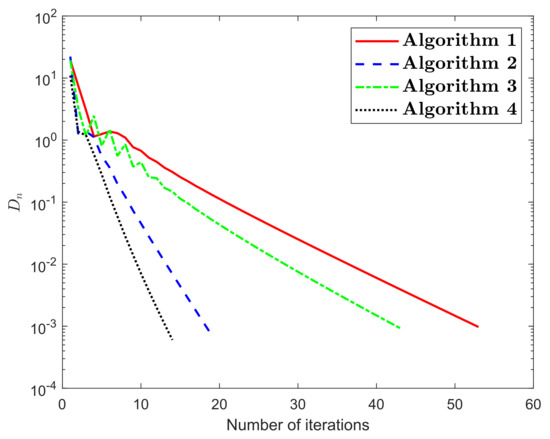
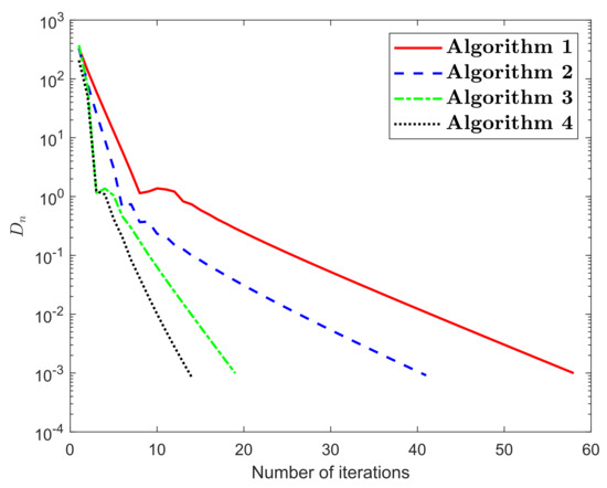
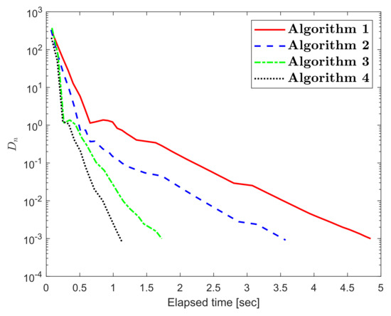
The numerical results for Example 1 are shown in Figure 1, Figure 2, Figure 3, Figure 4, Figure 5 and Figure 6 and Table 1Table 2. The control conditions are taken in the following way:

Figure 1. Numerical illustration of Algorithms 1–4 while $u_1=(1,1,\cdots ,1_{5000},0,0,\cdots ).$

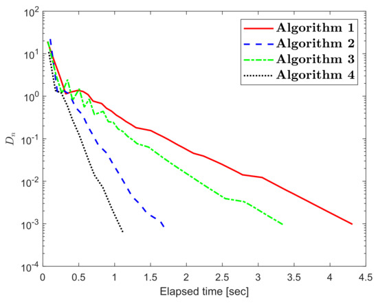
Figure 2. Numerical illustration of Algorithms 1–4 while $u_1=(1,1,\cdots ,1_{5000},0,0,\cdots ).$

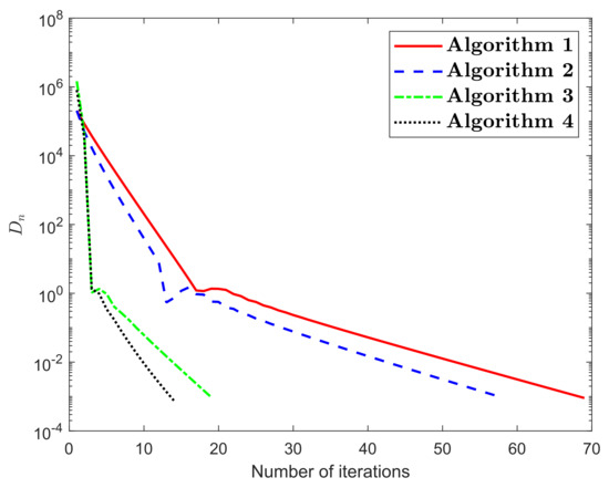
Figure 3. Numerical illustration of Algorithms 1–4 while $u_1=(1,2,\cdots ,5000,0,0,\cdots ).$

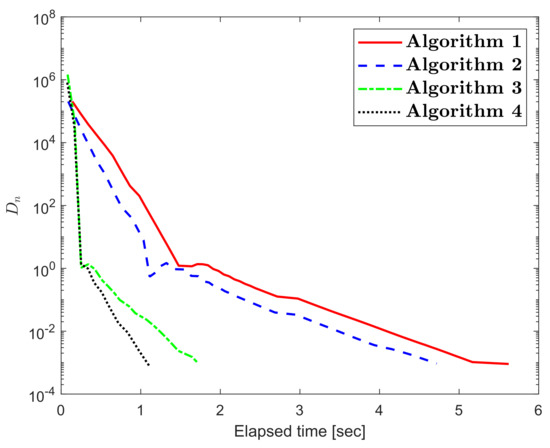
Figure 4. Numerical illustration of Algorithms 1–4 while $u_1=(1,2,\cdots ,5000,0,0,\cdots ).$

Figure 5. Numerical illustration of Algorithms 1–4 while $u_1=(5,5,\cdots ,5_{5000},0,0,\cdots ).$

Figure 6. Numerical illustration of Algorithms 1–4 while $u_1=(5,5,\cdots ,5_{5000},0,0,\cdots ).$

Table 1. Numerical values for Example 1.

	Number of Iterations		Execution Time in Seconds
${\mathbf{u}}_{\mathbf{1}}$	Algorithm 1	Algorithm 3	Algorithm 1	Algorithm 3
$(1,1,\cdots ,1_{5000},0,0,\cdots )$	53	43	4.31228480000000	3.35517350000000
$(1,2,\cdots ,5000,0,0,\cdots )$	69	58	5.62310790000000	4.71896740000000
$(5,5,\cdots ,5_{10000},0,0,\cdots )$	58	41	4.84570940000000	3.57478350000000

Table 2. Numerical values for Example 1.

	Number of Iterations		Execution Time in Seconds
${\mathbf{u}}_{\mathbf{0}}={\mathbf{u}}_{\mathbf{1}}$	Algorithm 2	Algorithm 4	Algorithm 2	Algorithm 4
$(1,1,\cdots ,1_{5000},0,0,\cdots )$	19	14	1.71126830000000	1.12075030000000
$(1,2,\cdots ,5000,0,0,\cdots )$	19	14	1.71955850000000	1.11015910000000
$(5,5,\cdots ,5_{10000},0,0,\cdots )$	19	14	1.72444340000000	1.12638850000000

(i)

Algorithm 1 (shortly, Algorithm 1):

$${\gamma }_1=0.22,\mu =0.44,{\beta }_n=\frac{1}{(n+2)},{\alpha }_n=\frac{1}{2}(1-{\beta }_n);$$

(ii)

Algorithm 3 (shortly, Algorithm 3):

$${\gamma }_1=0.22,\mu =0.44,{\beta }_n=\frac{1}{(n+2)},{\alpha }_n=\frac{1}{2}(1-{\beta }_n),{\phi }_n=\frac{100}{{(n+1)}^2};$$

(iii)

Algorithm 2 (shortly, Algorithm 2):

$${\gamma }_1=0.22,\mu =0.44,\rho =0.50,{\beta }_n=\frac{1}{(n+2)},{ϵ}_n=\frac{1}{{(n+1)}^2};$$

(iv)

Algorithm 4 (shortly, Algorithm 4):

$${\gamma }_1=0.22,\mu =0.44,\rho =0.50,{\beta }_n=\frac{1}{(n+2)},{ϵ}_n=\frac{1}{{(n+1)}^2},{\phi }_n=\frac{100}{{(n+1)}^2}.$$

5. Conclusions

We formulated four explicit extragradient-type methods to find a numerical solution to the quasimonotone variational inequalities in a real Hilbert space. These methods are considered as a modification of the two-step extragradient-type method. Two strongly convergent results have been proven corresponding to the proposed methods. The numerical results were examined in order to verify the numerical advantage of the proposed algorithms. Such computational results show that the non-monotone variable step size rule continues to improve the effectiveness of the iterative sequence in this context.

References

- Stampacchia, G. Formes bilinéaires coercitives sur les ensembles convexes. C. R. Hebd. Seances Acad. Sci. 1964, 258, 4413–4416. [Google Scholar]
- Konnov, I.V. On systems of variational inequalities. Rus. Math. Izvestiia-Vysshie Uchebnye Zavedeniia Matematika 1997, 41, 77–86. [Google Scholar]
- Kassay, G.; Kolumbán, J.; Páles, Z. On Nash stationary points. Publ. Math. 1999, 54, 267–279. [Google Scholar]
- Kassay, G.; Kolumbán, J.; Páles, Z. Factorization of Minty and Stampacchia variational inequality systems. Eur. J. Oper. Res. 2002, 143, 377–389. [Google Scholar] [CrossRef]
- Kinderlehrer, D.; Stampacchia, G. An Introduction to Variational Inequalities and Their Applications; Society for Industrial and Applied Mathematics: Philadelphia, PA, USA, 2000. [Google Scholar] [CrossRef]
- Konnov, I. Equilibrium Models and Variational Inequalities; Elsevier: Amsterdam, The Netherlands, 2007; Volume 210. [Google Scholar]
- Elliott, C.M. Variational and Quasivariational Inequalities Applications to Free—Boundary ProbLems. (Claudio Baiocchi And António Capelo). SIAM Rev. 1987, 29, 314–315. [Google Scholar] [CrossRef]
- Nagurney, A.; Economics, E.N. A Variational Inequality Approach; Springer: Berlin, Germany, 1999. [Google Scholar]
- Takahashi, W. Introduction to Nonlinear and Convex Analysis; Yokohama Publishers: Yokohama, Japan, 2009. [Google Scholar]
- Argyros, I.K.; Magreñán, Á. Iterative Methods and Their Dynamics with Applications; CRC Press: Boca Raton, FL, USA, 2017. [Google Scholar] [CrossRef]
- Argyros, I.K.; Magreñán, Á.A. Iterative Algorithms II; Nova Science Publishers: Hauppauge, NY, USA, 2016. [Google Scholar]
- Argyros, I.K.; Magreñán, Á.A. On the convergence of an optimal fourth-order family of methods and its dynamics. Appl. Math. Comput. 2015, 252, 336–346. [Google Scholar] [CrossRef]
- Argyros, I.K.; Magreñán, Á.A. Extending the convergence domain of the Secant and Moser method in Banach Space. J. Comput. Appl. Math. 2015, 290, 114–124. [Google Scholar] [CrossRef]
- Rehman, H.; Kumam, P.; Abubakar, A.B.; Cho, Y.J. The extragradient algorithm with inertial effects extended to equilibrium problems. Comput. Appl. Math. 2020, 39. [Google Scholar] [CrossRef]
- Rehman, H.; Kumam, P.; Kumam, W.; Shutaywi, M.; Jirakitpuwapat, W. The inertial sub-gradient extra-gradient method for a class of pseudo-monotone equilibrium problems. Symmetry 2020, 12, 463. [Google Scholar] [CrossRef] [Green Version]
- Rehman, H.; Kumam, P.; Argyros, I.K.; Deebani, W.; Kumam, W. Inertial extra-gradient method for solving a family of strongly pseudomonotone equilibrium problems in real Hilbert spaces with application in variational inequality problem. Symmetry 2020, 12, 503. [Google Scholar] [CrossRef] [Green Version]
- Rehman, H.; Kumam, P.; Argyros, I.K.; Alreshidi, N.A.; Kumam, W.; Jirakitpuwapat, W. A self-adaptive extra-gradient methods for a family of pseudomonotone equilibrium programming with application in different classes of variational inequality problems. Symmetry 2020, 12, 523. [Google Scholar] [CrossRef] [Green Version]
- Rehman, H.; Kumam, P.; Argyros, I.K.; Shutaywi, M.; Shah, Z. Optimization based methods for solving the equilibrium problems with applications in variational inequality problems and solution of Nash equilibrium models. Mathematics 2020, 8, 822. [Google Scholar] [CrossRef]
- Rehman, H.; Kumam, P.; Shutaywi, M.; Alreshidi, N.A.; Kumam, W. Inertial optimization based two-step methods for solving equilibrium problems with applications in variational inequality problems and growth control equilibrium models. Energies 2020, 13, 3292. [Google Scholar] [CrossRef]
- Korpelevich, G. The extragradient method for finding saddle points and other problems. Matecon 1976, 12, 747–756. [Google Scholar]
- Censor, Y.; Gibali, A.; Reich, S. The subgradient extragradient method for solving variational inequalities in Hilbert space. J. Optim. Theory Appl. 2010, 148, 318–335. [Google Scholar] [CrossRef] [Green Version]
- Censor, Y.; Gibali, A.; Reich, S. Strong convergence of subgradient extragradient methods for the variational inequality problem in Hilbert space. Optim. Methods Softw. 2011, 26, 827–845. [Google Scholar] [CrossRef]
- Censor, Y.; Gibali, A.; Reich, S. Extensions of Korpelevich extragradient method for the variational inequality problem in Euclidean space. Optimization 2012, 61, 1119–1132. [Google Scholar] [CrossRef]
- Tseng, P. A Modified Forward-Backward Splitting Method for Maximal Monotone Mappings. SIAM J. Control Optim. 2000, 38, 431–446. [Google Scholar] [CrossRef]
- Moudafi, A. Viscosity Approximation Methods for Fixed-Points Problems. J. Math. Anal. Appl. 2000, 241, 46–55. [Google Scholar] [CrossRef] [Green Version]
- Zhang, L.; Fang, C.; Chen, S. An inertial subgradient-type method for solving single-valued variational inequalities and fixed point problems. Numer. Algorithms 2018, 79, 941–956. [Google Scholar] [CrossRef]
- Iusem, A.N.; Svaiter, B.F. A variant of korpelevich’s method for variational inequalities with a new search strategy. Optimization 1997, 42, 309–321. [Google Scholar] [CrossRef]
- Bauschke, H.H.; Combettes, P.L. Convex Analysis and Monotone Operator Theory in Hilbert Spaces; Springer: Berlin, Germany, 2011; Volume 408. [Google Scholar]
- Xu, H.K. Another control condition in an iterative method for nonexpansive mappings. Bull. Aust. Math. Soc. 2002, 65, 109–113. [Google Scholar] [CrossRef] [Green Version]
- Maingé, P.E. Strong Convergence of Projected Subgradient Methods for Nonsmooth and Nonstrictly Convex Minimization. Set-Valued Anal. 2008, 16, 899–912. [Google Scholar] [CrossRef]
Publisher’s Note: MDPI stays neutral with regard to jurisdictional claims in published maps and institutional affiliations. |
© 2021 by the authors. Licensee MDPI, Basel, Switzerland. This article is an open access article distributed under the terms and conditions of the Creative Commons Attribution (CC BY) license (https://creativecommons.org/licenses/by/4.0/).