Non-Isothermal Creeping Flows in a Pipeline Network: Existence Results

Abstract

This paper deals with a 3D mathematical model for the non-isothermal steady-state flow of an incompressible fluid with temperature-dependent viscosity in a pipeline network. Using the pressure and heat flux boundary conditions, as well as the conjugation conditions to satisfy the mass balance in interior junctions of the network, we propose the weak formulation of the nonlinear boundary value problem that arises in the framework of this model. The main result of our work is an existence theorem (in the class of weak solutions) for large data. The proof of this theorem is based on a combination of the Galerkin approximation scheme with one result from the field of topological degrees for odd mappings defined on symmetric domains.

1. Introduction and Problem Formulation

At the current time, pipeline networks of complex geometry, including main pipeline networks, are extensively applied to liquids and gases transfer [1,2,3,4]. Many authors have studied various problems involving mathematical modeling of the transportation of liquids and gases. Panasenko [5,6] investigated the Navier–Stokes network problem stated in the so-called thin structure, i.e., in a network of thin tubes with the ratio of the cross-section diameter to the height of order $\epsilon \ll 1$. Asymptotic analysis of the non-steady Navier–Stokes equations in such structures is given in [7,8]. A nonlinear one-dimensional model for the stationary motion of a non-Newtonian fluid in the thin structure is studied in [9]. Banda et al. [10] introduced a model for the gas flow in pipeline networks based on the isothermal Euler equations and proposed a method to obtain numerical solutions of the gas network problem for sample networks. Herty and Seaïd [11] numerically investigated a well-established model for gas flows in pipeline networks using suitable coupling conditions at pipe-to-pipe fittings. Colombo and Garavello [12] considered the generalized Riemann problem for the p-system at a junction connecting n ducts and proved the existence and uniqueness of stationary solutions and of their perturbations. Colombo et al. [13] presented a unified approach for $2\times 2$ conservation laws at a junction and established the well-posedness of the corresponding Cauchy problem. Their construction comprehends the cases of one-dimensional isothermal models for gas flows and the shallow-water equations for flows in open channels. Herty et al. [14] introduced a model for gas dynamics in pipe networks assuming that the gravity and inertia effects are neglectable, both justifiable simplifications for the gas flow in pipelines. The derived equations are obtained by asymptotic analysis in the pressure variable. Colombo and Mauri [15] proved the well-posedness of the Cauchy problem for the compressible Euler system at a junction. Chalons et al. [16] investigated the one-dimensional coupling of two systems of gas dynamics at a fixed interface. Banda et al. [17] performed the mathematical analysis of multiphase flows through networks under assumption that the flow through the connected arcs is governed by an isothermal no-slip drift-flux model. Marušić-Paloka [18] presented some results about asymptotic approximations of the incompressible viscous flow through a network of intersected thin pipes with the prescribed pressure at their ends. Sagadeeva and Sviridyuk [19] proposed a linear approximation of a model for oil transportation in a pipeline network and investigated the stability and the optimal control of solutions for the appropriate system of partial differential equations. Reigstad [20] analyzed a network model for junction flows that are governed by the one-dimensional isentropic Euler equations. Aida-zade and Ashrafova [21] numerically solved an inverse problem for a pipeline network with loopback structure using non-separated boundary conditions. In the paper [22], an optimal control problem for the linearized Navier–Stokes system with distributed parameters in a net-like domain is studied. Holle et al. [23] introduced new coupling conditions for the isentropic flow on networks based on an artificial density at the junction. Baranovskii [24] proposed a network model that describes the isothermal steady-state 3D flow of an incompressible non-Newtonian fluid with shear-dependent viscosity and proved an existence theorem in the class of weak solutions to the corresponding boundary value problem. The recent papers [25,26,27,28] are devoted to the analysis of viscous flows and heat transfer in channels and tubes.

Despite the large number of works, the mathematical theory of heat and mass transfer in pipeline networks is very far from complete and most of the theoretical results were obtained for networks with a simplified geometry. Important challenges in this field are the development and analysis of multi-dimensional nonlinear models describing non-isothermal viscous flows in pipeline networks subject to the conjugation conditions in junctions. In the conference paper [29], we obtained the existence results for one such model under the assumption that the data are sufficiently small. The present paper is a continuation of this study. Namely, we shall consider here a mathematical model that describes the non-isothermal creeping flow in a net-like domain $\tilde{\mathcal{P}}=\mathcal{P}\cup \mathfrak{J}$:

$$\mathcal{P}=\bigcup _{i=1}^N{\mathcal{P}}_i,\mathfrak{J}=\bigcup _{\ell =1}^M{\mathfrak{J}}_{\ell },$$

where ${\mathcal{P}}_i$ and ${\mathfrak{J}}_{\ell }$ are bounded domains in space ${\mathbb{R}}^3$ with Lipschitz-continuous boundaries and

$$\begin{array}{cc}\hfill {\overline{\mathcal{P}}}_i& \cap {\overline{\mathcal{P}}}_k=⌀,\forall i,k\in \{1,2,\cdots ,N\}\text{such that} i\ne k,\hfill \\ \hfill {\overline{\mathfrak{J}}}_{\ell }& \cap {\overline{\mathfrak{J}}}_s=⌀,\forall \ell ,s\in \{1,2,\cdots ,M\}\text{such that} \ell \ne s,\hfill \\ \hfill {\mathcal{P}}_i& \cap {\mathfrak{J}}_{\ell }=⌀,\forall i\in \{1,2,\cdots ,N\},\ell \in \{1,2,\cdots ,M\}.\hfill \end{array}$$

The domain $\tilde{\mathcal{P}}$ can be considered as a network of pipes:

• ${\mathcal{P}}_1$, …, ${\mathcal{P}}_N$ model pipes;
• ${\mathfrak{J}}_1$, …, ${\mathfrak{J}}_M$ represent junctions in which pipes are connected.

Following ideas from [24], we introduce some assumptions about the geometry of the domain $\tilde{\mathcal{P}}$.

(A1)

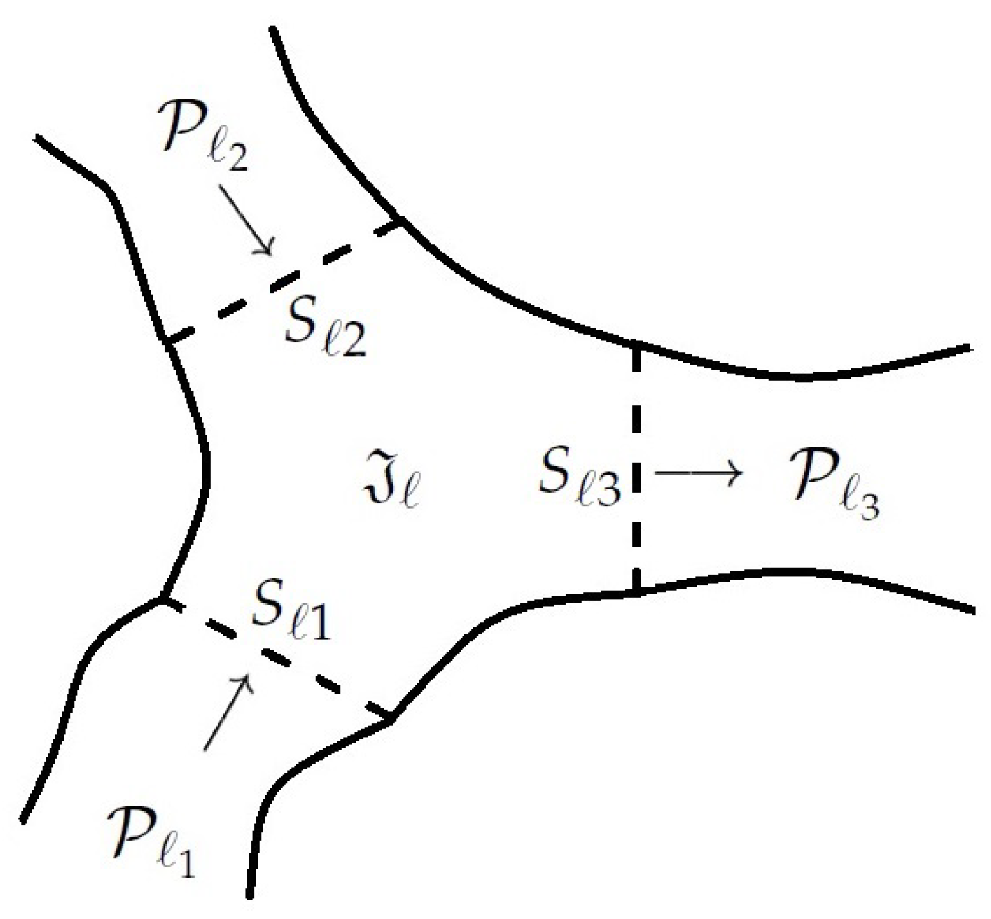
For each junction ${\mathfrak{J}}_{\ell }$ there exist exactly $m_{\ell }$ pipes ${\mathcal{P}}_{{\ell }_1}$, ${\mathcal{P}}_{{\ell }_2}$, ..., ${\mathcal{P}}_{{\ell }_{m_{\ell }}}$, where $1\le m_{\ell }\le N$ and $1\le {\ell }_1<{\ell }_2<\cdots <{\ell }_{m_{\ell }}\le N$, such that

$${\overline{\mathfrak{J}}}_{\ell }\cap {\overline{\mathcal{P}}}_{{\ell }_k}\ne ⌀,\forall k\in \{1,2,\cdots ,m_{\ell }\}.$$

(A2)

The intersection $S_{\ell n}\stackrel{\text{def}}{=}{\overline{\mathfrak{J}}}_{\ell }\cap {\overline{\mathcal{P}}}_{{\ell }_n}$ is a flat surface, for any $\ell \in \{1,2,\cdots ,M\}$ and $n\in \{1,2,\cdots ,m_{\ell }\}$.

(A3)

For each pipe ${\mathcal{P}}_i$ there exist exactly two junctions ${\mathfrak{J}}_{i_1}$ and ${\mathfrak{J}}_{i_2}$ such that

$${\overline{\mathcal{P}}}_i\cap {\overline{\mathfrak{J}}}_{i_1}\ne ⌀,{\overline{\mathcal{P}}}_i\cap {\overline{\mathfrak{J}}}_{i_2}\ne ⌀.$$

If $m_{\ell }\ge 2$ in condition (A1), then we shall say that the junction ${\mathfrak{J}}_{\ell }$ is interior; in the case $m_{\ell }=1$, the junction ${\mathfrak{J}}_{\ell }$ is called external.

From condition (A3) it follows that for each $i\in \{1,2,\cdots ,N\}$ there exists a uniquely determined pair $(i_1^{\prime },i_2^{\prime })$ such that

$${\overline{\mathcal{P}}}_i\cap {\overline{\mathfrak{J}}}_{i_1}=S_{i_1{i}_1^{\prime }},{\overline{\mathcal{P}}}_i\cap {\overline{\mathfrak{J}}}_{i_2}=S_{i_2{i}_2^{\prime }}.$$

Let us introduce the following notation:

$$\begin{array}{c}{{\Gamma }}_i\stackrel{\text{def}}{=}\partial {\mathcal{P}}_i\backslash (S_{i_1{i}_1^{\prime }}\cup S_{i_2{i}_2^{\prime }}),i=1,2,\cdots ,N,\\ {\Gamma }\stackrel{\text{def}}{=}\bigcup _{i=1}^N{{\Gamma }}_i,S\stackrel{\text{def}}{=}\bigcup _{\ell =1}^M\bigcup _{n=1}^{m_{\ell }}{S}_{\ell n}.\end{array}$$

Examples of network sections are given in Figure 1 and Figure 2.

Figure 1. The pipe ${\mathcal{P}}_i$ and the junctions ${\mathfrak{J}}_{i_1}$ and ${\mathfrak{J}}_{i_2}$.

Figure 2. The interior junction ${\mathfrak{J}}_{\ell }$ and the pipes ${\mathcal{P}}_{{\ell }_1}$, ${\mathcal{P}}_{{\ell }_2}$, ${\mathcal{P}}_{{\ell }_3}$.

Consider a stationary mathematical model for non-isothermal creeping flows in the pipeline network $\mathcal{P}$:

$$-\nabla ·\left[\mu \left(\theta \right)\mathbb{D}\left(\mathit{u}\right)\right]+\nabla \pi ={\mathit{f}}_i(\mathit{x},\theta )\text{in} {\mathcal{P}}_i,i=1,2,\cdots ,N,$$

(1)

$$\nabla ·\mathit{u}=0\text{in} \mathcal{P},$$

(2)

$$(\mathit{u}·\nabla )\theta -\kappa {\Delta }\theta ={\phi }_i(\mathit{x},\theta )\text{in} {\mathcal{P}}_i,i=1,2,\cdots ,N,$$

(3)

$$\mathit{u}=\mathbf{0}\text{on} {\Gamma },$$

(4)

$$\kappa \frac{\partial \theta }{\partial \mathbf{n}}=-{\beta }_i\theta \text{on} {{\Gamma }}_i,i=1,2,\cdots ,N,$$

(5)

$${\mathit{u}}_{\tan }=\mathbf{0}\text{on} S,$$

(6)

$$\pi ={\pi }_i\text{on} S_{i_1{i}_1^{\prime }}\cup S_{i_2{i}_2^{\prime }},i=1,2,\cdots ,N,$$

(7)

$$\frac{\theta }{2}(\mathit{u}·\mathbf{n})-\kappa \frac{\partial \theta }{\partial \mathbf{n}}={\psi }_i(\mathit{x},\theta ,\mathit{u})\text{on} S_{i_1{i}_1^{\prime }}\cup S_{i_2{i}_2^{\prime }},i=1,2,\cdots ,N,$$

(8)

$$\sum _{k=1}^{m_{\ell }}\underset{S_{\ell k}}{\int }\mathit{u}·\mathbf{n}dS=0\text{for each} \ell \in \{1,2,\cdots ,M\}\text{such that} m_{\ell }\ge 2,$$

(9)

where $\mathit{u}$ is the velocity field; $\pi$ is the pressure; $\theta$ is the temperature; ${\mathit{f}}_i$ stands for the external force that is applied to the fluid filling the pipe ${\mathcal{P}}_i$; $\mu \left(\theta \right)>0$ represents the viscosity of the fluid; $\kappa >0$ is the thermal conductivity; ${\phi }_i$ denotes the heat source intensity for the pipe ${\mathcal{P}}_i$; ${\beta }_i>0$ is the Robin coefficient characterizing the heat transfer on the wall ${{\Gamma }}_i$; the functions ${\pi }_i$ and ${\psi }_i$ describe, respectively, the pressure and the heat fluxes on the surface $S_{i_1{i}_1^{\prime }}\cup S_{i_2{i}_2^{\prime }}$. By $\mathbf{n}$ we denote the outer (with respect to the pipe ${\mathcal{P}}_i$) unit normal to $\partial {\mathcal{P}}_i$. As usual, the subscript notation “tan” indicates the tangential component of a vector, i.e., ${\mathit{v}}_{\tan }\stackrel{\text{def}}{=}\mathit{v}-(\mathit{v}·\mathbf{n})\mathbf{n}$. The term $dS$ denotes infinitesimal surface element of S. The symbol ∇ stands for the gradient with respect to the space variables $x_1$, $x_2$, $x_3$ and

$$\begin{array}{c}\nabla \mathit{v}\stackrel{\text{def}}{=}\left[\begin{array}{ccc}{\displaystyle \frac{\partial v_1}{\partial x_1}}& {\displaystyle \frac{\partial v_1}{\partial x_2}}& {\displaystyle \frac{\partial v_1}{\partial x_3}}\\ {\displaystyle \frac{\partial v_2}{\partial x_1}}& {\displaystyle \frac{\partial v_2}{\partial x_2}}& {\displaystyle \frac{\partial v_2}{\partial x_3}}\\ {\displaystyle \frac{\partial v_3}{\partial x_1}}& {\displaystyle \frac{\partial v_3}{\partial x_2}}& {\displaystyle \frac{\partial v_3}{\partial x_3}}\end{array}\right],\nabla ·\mathit{F}\stackrel{\text{def}}{=}\left(\begin{array}{c}{\displaystyle \sum _{i=1}^3}{\displaystyle \frac{\partial F_{i1}}{\partial x_i}}\\ {\displaystyle \sum _{i=1}^3}{\displaystyle \frac{\partial F_{i2}}{\partial x_i}}\\ {\displaystyle \sum _{i=1}^3}{\displaystyle \frac{\partial F_{i3}}{\partial x_i}}\end{array}\right),\\ \nabla ·\mathit{v}\stackrel{\text{def}}{=}\sum _{i=1}^3{\displaystyle \frac{\partial v_i}{\partial x_i}},\mathbb{D}\left(\mathit{v}\right)\stackrel{\text{def}}{=}\frac{1}{2}\left(\nabla \mathit{v}+{(\nabla \mathit{v})}^{\top }\right),\end{array}$$

for a vector function $\mathit{v}=(v_1,v_2,v_3)$ and a matrix-valued function $\mathit{F}={\left(F_{ij}\right)}_{i=1,j=1}^{3,3}$.

In model (1)–(9), the unknowns are $\mathit{u}$, $\theta$, and $\pi$, while all other quantities are prescribed. Note that (1) is the balance of linear momentum under assumption that inertial effects are neglected, i.e., we consider the so-called Stokes flow in which the inertia is negligible compared to viscous and pressure forces. Equation (2) is the incompressibility condition, (3) is the energy balance, relation (4) is the no-slip boundary condition on walls of pipes, and (5) is Newton’s law of cooling. Boundary conditions (6)–(8) govern the fluid flow and the heat flux through components of S. Finally, relation (9) is the conjugation condition that represents the mass balance for interior junctions of the network $\tilde{\mathcal{P}}$.

The main aim of this paper is to prove the solvability of boundary value problem (1)–(9) in the weak formulation under mild assumptions on the data. In order to establish the existence of weak solutions, we use the Galerkin approximation scheme and one result (see Proposition 1) from the field of topological degrees. The proof is based on the energy estimates of approximate solutions in Sobolev spaces, the Krasnoselskii theorem on the continuity of the Nemytskii superposition operator in Lebesgue spaces as well as the compactness theorems for the imbedding and trace operators.

The paper is organized as follows. In the next section, we introduce the main notation and function spaces, as well as some assumptions on the model data. Section 3 is devoted to the functional setting of boundary value problem (1)–(9). In this section we also formulate the central result of the paper, the Theorem 1 on the existence and some properties of weak solutions. Finally, Section 4 deals with the proof of Theorem 1.

2. Preliminaries: Main Notation, Function Spaces, and Assumptions

For the reader’s convenience, mostly standard notation is used.

By ${\mathrm{meas}}_n(·)$ denote the Lebesgue n-dimensional measure of a set.

For matrices $\mathit{X}={\left(X_{ij}\right)}_{k=i,j=1}^{n,n}$ and $\mathit{Y}={\left(Y_{ij}\right)}_{i=1,j=1}^{n,n}$, by $\mathit{X}:\mathit{Y}$ denote the component-wise matrix product, i.e.,

$$\mathit{X}:\mathit{Y}\stackrel{\text{def}}{=}\sum _{i,j=1}^n{X}_{ij}{Y}_{ij}.$$

By $\left|\mathit{x}\right|$ denote the Euclidean norm of a vector $\mathit{x}=(x_1,\cdots ,x_n)$ and by $\left|\mathit{X}\right|$ denote the Frobenius norm of a matrix $\mathit{X}$:

$${\left|\mathit{x}\right|}^2\stackrel{\text{def}}{=}\mathit{x}·\mathit{x}=\sum _{i=1}^n{x}_i^2,{\left|\mathit{X}\right|}^2\stackrel{\text{def}}{=}\mathit{X}:\mathit{X}=\sum _{i,j=1}^n{X}_{ij}^2.$$

We shall use the Lebesgue space $L^p\left({\Omega }\right)$, where ${\Omega }$ is a bounded Lipschitz domain in ${\mathbb{R}}^3$ and $p\in [1,\infty )$, with the norm

$${\parallel v\parallel }_{L^p\left({\Omega }\right)}\stackrel{\text{def}}{=}{\left(\underset{{\Omega }}{\int }{\left|v\right|}^p\mathit{dx}\right)}^{1/p}$$

and the Sobolev space $H^1\left({\Omega }\right)\stackrel{\text{def}}{=}{W}^{1,2}\left({\Omega }\right),$ which is equipped with the norm

$${\parallel v\parallel }_{H^1\left({\Omega }\right)}\stackrel{\text{def}}{=}{\left(\underset{{\Omega }}{\int }{\left|v\right|}^2\mathit{dx}+\underset{{\Omega }}{\int }{|\nabla v|}^2\mathit{dx}\right)}^{1/2};$$

see [30] for definitions of these spaces and the systematic description of their properties. For the sake of brevity, we shall denote the corresponding spaces of vector-valued functions by using bold face letters, i.e.,

$$\begin{array}{cc}\hfill {\mathit{L}}^p\left({\Omega }\right)& \stackrel{\text{def}}{=}{L}^p\left({\Omega }\right)\times L^p\left({\Omega }\right)\times L^p\left({\Omega }\right),\hfill \\ \hfill {\mathit{H}}^1\left({\Omega }\right)& \stackrel{\text{def}}{=}{H}^1\left({\Omega }\right)\times H^1\left({\Omega }\right)\times H^1\left({\Omega }\right).\hfill \end{array}$$

Recall that the restriction of a function $v\in H^1\left({\Omega }\right)$ to the surface $\partial {\Omega }$ is defined by the formula ${v|}_{\partial {\Omega }}=\gamma v$, where $\gamma :H^1\left({\Omega }\right)\to L^4(\partial {\Omega })$ is the trace operator (see [31], § 2.4.2).

By definition, put

$$\begin{array}{cc}\hfill \mathcal{V}\left(\mathcal{P}\right)\stackrel{\text{def}}{=}\{\mathit{w}:\overline{\mathcal{P}}\to {\mathbb{R}}^3:& {\mathit{w}|}_{{\overline{\mathcal{P}}}_i}\in {\mathbf{C}}^{\infty }\left({\overline{\mathcal{P}}}_i\right)\text{for each} i=1,2,\cdots ,N \text{and} \hfill \end{array}$$

                                                                             ω satisfies (2), (4), (6) and (9)}.

We introduce the space $\mathit{V}\left(\mathcal{P}\right)$ defined as

$$\mathit{V}\left(\mathcal{P}\right)\stackrel{\text{def}}{=}\text{the closure of the set} \mathcal{V}\left(\mathcal{P}\right)\text{in the Sobolev space} {\mathit{H}}^1\left(\mathcal{P}\right)$$

with the scalar product

$${(\mathit{u},\mathit{v})}_{\mathit{V}\left(\mathcal{P}\right)}\stackrel{\text{def}}{=}\sum _{i=1}^N\underset{{\mathcal{P}}_i}{\int }\mathbb{D}\left(\mathit{u}\right):\mathbb{D}\left(\mathit{v}\right)\mathit{dx}.$$

Note that the associated norm

$${\parallel ·\parallel }_{\mathit{V}\left(\mathcal{P}\right)}\stackrel{\text{def}}{=}{(·,·)}_{\mathit{V}\left(\mathcal{P}\right)}^{1/2}$$

is equivalent to the norm induced from the Sobolev space ${\mathit{H}}^1\left(\mathcal{P}\right)$. This follows from Korn’s inequality.

Lemma 1

(Korn’s inequality). Suppose ${\Omega }$ is a bounded domain in space ${\mathbb{R}}^3$ with boundary $\partial {\Omega }\in C^{0,1}$. If ${\Sigma }\subset \partial {\Omega }$ and ${\mathrm{meas}}_2\left({\Sigma }\right)>0$, then there exists a positive constant $C=C\left({\Omega }\right)$ such that the following inequality

$${\parallel \mathbb{D}\left(\mathit{v}\right)\parallel }_{{\mathit{L}}^2\left({\Omega }\right)}\ge C\left({\Omega }\right){\parallel \mathit{v}\parallel }_{{\mathit{H}}^1\left({\Omega }\right)}$$

holds for all $\mathit{v}\in {\mathit{H}}^1\left({\Omega }\right)$ satisfying the boundary condition ${\mathit{v}|}_{{\Sigma }}=\mathit{0}$.

This lemma is a consequence of Theorems 2.2 and 2.3 that is given in [32], Chapter I.

Further, introduce the space $W\left(\mathcal{P}\right)$ defined as

$$W\left(\mathcal{P}\right)\stackrel{\text{def}}{=}\left\{\theta :\overline{\mathcal{P}}{\to \mathbb{R}:\theta |}_{{\mathcal{P}}_i}\in H^1\left({\mathcal{P}}_i\right)\text{for each} i=1,2,\cdots ,N\right\}$$

with the scalar product

$${(\theta ,\xi )}_{W\left(\mathcal{P}\right)}\stackrel{\text{def}}{=}\kappa \sum _{i=1}^N\underset{{\mathcal{P}}_i}{\int }\nabla \theta ·\nabla \xi \mathit{dx}+\sum _{i=1}^N{\beta }_i\underset{{{\Gamma }}_i}{\int }\theta \xi d{\Gamma }.$$

Since ${\mathrm{meas}}_2\left({{\Gamma }}_i\right)>0$ for each $i\in \{1,2,\cdots ,N\}$, it can be proved that the associated norm

$${\parallel ·\parallel }_{W\left(\mathcal{P}\right)}={(·,·)}_{W\left(\mathcal{P}\right)}^{1/2}$$

is equivalent to the norm ${\parallel ·\parallel }_{H^1\left(\mathcal{P}\right)}$.

Let us now describe the conditions that are imposed on the data of problem (1)–(9).

(B1)

The function $\mu :\mathbb{R}\to \mathbb{R}$ is continuous.

(B2)

There exist constants ${\mu }_0$ and ${\mu }_1$ such that

$$0<{\mu }_0\le \mu \left(r\right)\le {\mu }_1,\forall r\in \mathbb{R}.$$

(B3)

The functions ${\mathit{f}}_i(·,r):\mathcal{P}\to {\mathbb{R}}^3$, ${\phi }_i(·,r):\mathcal{P}\to \mathbb{R}$, ${\psi }_i(·,r,\mathit{y}):\mathcal{P}\to \mathbb{R}$ are measurable for any $i\in \{1,2,\cdots ,N\}$, $r\in \mathbb{R}$, $\mathit{y}\in {\mathbb{R}}^3$.

(B4)

The functions ${\mathit{f}}_i(\mathit{x},·):\mathbb{R}\to {\mathbb{R}}^3$, ${\phi }_i(\mathit{x},·):\mathbb{R}\to \mathbb{R}$, ${\psi }_i(\mathit{x},·,·):\mathbb{R}\times {\mathbb{R}}^3\to \mathbb{R}$ are continuous for each $i\in \{1,2,\cdots ,N\}$ and almost every $\mathit{x}\in \mathcal{P}$.

(B5)

There exist constants $K_f$, $K_{\phi }$, $K_{\psi }$ such that

$$|{\mathit{f}}_i(\mathit{x},r)|\le K_f,|{\phi }_i(\mathit{x},r)|\le K_{\phi },\left|{\psi }_i(\mathit{x},r,\mathit{y})\right|\le K_{\psi },\forall i\in \{1,2,\cdots ,N\},$$

for almost every $\mathit{x}\in \mathcal{P}$ and for any $r\in \mathbb{R}$ and $\mathit{y}\in {\mathbb{R}}^3$.

(B6)

The function ${\pi }_i:S_{i_1{i}_1^{\prime }}\cup S_{i_2{i}_2^{\prime }}\to \mathbb{R}$ belongs to the Lebesgue space $L^2(S_{i_1{i}_1^{\prime }}\cup S_{i_2{i}_2^{\prime }})$ for each $i\in \{1,2,\cdots ,N\}$.

3. Functional Setting of the Problem and Main Results

In this section, we give the weak formulation of problem (1)–(9). We start with the following lemma, which suggests how to define a weak solution in a suitable way.

Lemma 2.

If $(\mathit{u},\theta ,\pi )$ is a classical solution to boundary value problem (1)–(9), then

$$\sum _{i=1}^N\underset{{\mathcal{P}}_i}{\int }\mu \left(\theta \right)\mathbb{D}\left(\mathit{u}\right):\mathbb{D}\left(\mathit{v}\right)\mathit{dx}+\sum _{i=1}^N\underset{S_{i_1{i}_1^{\prime }}\cup S_{i_2{i}_2^{\prime }}}{\int }{\pi }_i\mathit{v}·\mathbf{n}dS=\sum _{i=1}^N\underset{{\mathcal{P}}_i}{\int }{\mathit{f}}_i(\mathit{x},\theta )·\mathit{v}\mathit{dx},$$

(10)

$$\begin{array}{c}-\sum _{i=1}^N\sum _{k=1}^3\underset{{\mathcal{P}}_i}{\int }{u}_k\theta \frac{\partial \xi }{\partial x_k}\mathit{dx}+\kappa \sum _{i=1}^N\underset{{\mathcal{P}}_i}{\int }\nabla \theta ·\nabla \xi \mathit{dx}+\sum _{i=1}^N{\beta }_i\underset{{{\Gamma }}_i}{\int }\theta \xi d{\Gamma }\\ +\sum _{i=1}^N\underset{S_{i_1{i}_1^{\prime }}\cup S_{i_2{i}_2^{\prime }}}{\int }\left(\frac{\theta }{2}\mathit{u}·\mathit{n}+{\psi }_i(\mathit{x},\theta ,\mathit{u})\right)\xi dS=\sum _{i=1}^N\underset{{\mathcal{P}}_i}{\int }{\phi }_i(\mathit{x},\theta )\xi \mathit{dx}\end{array}$$

(11)

hold for any functions $\mathit{v}\in \mathit{V}\left(\mathcal{P}\right)$ and $\xi \in W\left(\mathcal{P}\right)$.

The proof of this lemma is much like that of Lemma 1 in [33] (see also [34], Remark 4) and, therefore, it will be omitted here.

Definition 1.

We shall say that a pair $(\mathit{u},\theta )\in \mathit{V}\left(\mathcal{P}\right)\times W\left(\mathcal{P}\right)$ is a weak solution of problem (1)–(9) if equalities (10) and (11) hold for any functions $\mathit{v}\in \mathit{V}\left(\mathcal{P}\right)$ and $\xi \in W\left(\mathcal{P}\right)$.

By $\mathfrak{M}$ denote the set of all weak solutions to problem (1)–(9).

Remark 1.

If a weak solution of system (1)–(9) is obtained, then one can find the velocity and temperature fields in interior junctions of the network $\tilde{\mathcal{P}}$ by solving the corresponding nonhomogeneous boundary value problems. Since the conjugation conditions (9) hold, these problems are well-posed.

We now formulate the main results of this paper.

Theorem 1.

Suppose conditions (A1)–(A3) and (B1)–(B6) hold. Then,

(i)

Boundary value problem (1)–(9)has at least one weak solution.

(ii)

Any weak solution $(\mathit{u},\theta )\in \mathit{V}\left(\mathcal{P}\right)\times W\left(\mathcal{P}\right)$ of problem (1)–(9) satisfies the following energy equalities:

$$\sum _{i=1}^N\underset{{\mathcal{P}}_i}{\int }\mu \left(\theta \right){\left|\mathbb{D}\left(\mathit{u}\right)\right|}^2\mathit{dx}+\sum _{i=1}^N\underset{S_{i_1{i}_1^{\prime }}\cup S_{i_2{i}_2^{\prime }}}{\int }{\pi }_i\mathit{u}·\mathbf{n}dS=\sum _{i=1}^N\underset{{\mathcal{P}}_i}{\int }{\mathit{f}}_i(\mathit{x},\theta )·\mathit{u}\mathit{dx},$$

(12)

$$\begin{array}{c}\kappa \sum _{i=1}^N\underset{{\mathcal{P}}_i}{\int }{|\nabla \theta |}^2\mathit{dx}+\sum _{i=1}^N\underset{S_{i_1{i}_1^{\prime }}\cup S_{i_2{i}_2^{\prime }}}{\int }{\psi }_i(\mathit{x},\theta ,\mathit{u})\theta dS+\sum _{i=1}^N{\beta }_i\underset{{{\Gamma }}_i}{\int }{\left|\theta \right|}^{2}d{\Gamma }\hfill \\ \hfill =\sum _{i=1}^N\underset{{\mathcal{P}}_i}{\int }{\phi }_i(\mathit{x},\theta )\theta \mathit{dx}.\end{array}$$

(13)

(iii)

If $({\mathit{u}}_1,\theta )\in \mathfrak{M}$ and $({\mathit{u}}_2,\theta )\in \mathfrak{M}$, then ${\mathit{u}}_1\equiv {\mathit{u}}_2$.

(iv)

The weak solutions set $\mathfrak{M}$ is sequentially weakly closed in the space $\mathit{V}\left(\mathcal{P}\right)\times W\left(\mathcal{P}\right)$.

The proof of this theorem is given in the next section.

4. Proof of Main Results

The following two propositions will be needed to prove Theorem 1.

Proposition 1.

Let ${\Omega }$ be an open bounded set in ${\mathbb{R}}^n$ such that

• the inclusion $\mathit{0}\in {\Omega }$ is valid;
• ${\Omega }$is symmetric in the following sense: if $\mathit{x}\in {\Omega }$, then $-\mathit{x}\in {\Omega }$.

Suppose $\mathbf{G}:\overline{{\Omega }}\times [0,1]\to {\mathbb{R}}^n$ is a continuous map and the following two conditions hold:

• $\mathbf{G}(\mathit{x},\lambda )\ne \mathit{0}$ for any pair $(\mathit{x},\lambda )\in \partial {\Omega }\times [0,1];$
• $\mathbf{G}(·,0):\overline{{\Omega }}\to {\mathbb{R}}^n$ is an odd mapping, i.e., $\mathbf{G}(-\mathit{x},0)=-\mathbf{G}(\mathit{x},0)$ for any vector $\mathit{x}\in \overline{{\Omega }}$.

Then, for any $\lambda \in [0,1]$ the equation $\mathbf{G}(\mathit{x},\lambda )=\mathit{0}$ has at least one solution ${\mathit{x}}_{\lambda }$, which belongs to the set${\Omega }$.

The proof of Proposition 1 is based on symmetry principles and topological degree methods (for details, see [35], Section 5).

Proposition 2.

Let $\mathcal{O}$ be a bounded domain in ${\mathbb{R}}^n$. Suppose $h:\mathcal{O}\times {\mathbb{R}}^d\to \mathbb{R}$ is a function such that

• the function $h(·,\mathit{y}):\mathcal{O}\to \mathbb{R}$ is measurable for every $\mathit{y}\in {\mathbb{R}}^d$;
• the function $h(\mathit{x},·):{\mathbb{R}}^d\to \mathbb{R}$ is continuous for almost every $\mathit{x}\in \mathcal{O}$;
• there exist constants $p_k,q\ge 1$, $\nu \ge 0$ and a function $\zeta \in L^q\left(\mathcal{O}\right)$ such that the inequality

  $$\left|h(\mathit{x},\mathit{y})\right|\le \zeta \left(\mathit{x}\right)+\nu \sum _{k=1}^d{\left|y_k\right|}^{p_k/q}$$
  holds for every $\mathit{y}\in {\mathbb{R}}^d$ and for almost every $\mathit{x}\in \mathcal{O}$.

Then the Nemytskii operator $N_h:L^{p_1}\left(\mathcal{O}\right)\times \cdots \times L^{p_d}\left(\mathcal{O}\right)\to L^q\left(\mathcal{O}\right)$ defined by

$$N_h[y_1,\cdots ,y_d]\left(\mathit{x}\right)\stackrel{\text{def}}{=}h(\mathit{x},y_1\left(\mathit{x}\right),\cdots ,y_d\left(\mathit{x}\right))$$

is a bounded and continuous map.

For the proof of Proposition 2, we refer the readers to the book [36], Chapter I.

First we shall establish the existence result (i). The proof will be achieved through three steps.

Step 1: The Galerkin approximation scheme.

Let ${\left\{{\mathit{v}}_{\ell }\right\}}_{\ell =1}^{\infty }$ be an orthonormal basis of the space $\mathit{V}\left(\mathcal{P}\right)$ and let ${\left\{{\xi }_{\ell }\right\}}_{\ell =1}^{\infty }$ be an orthonormal basis of the space $W\left(\mathcal{P}\right)$. Without loss of generality it can be assumed that

$${\left\{{\mathit{v}}_{\ell }\right\}}_{\ell =1}^{\infty }\subset \mathcal{V}\left(\mathcal{P}\right),{\left\{{\xi }_{\ell }\right\}}_{\ell =1}^{\infty }\subset C^{\infty }\left(\overline{\mathcal{P}}\right).$$

For an arbitrary fixed $m\in \mathbb{N}$, consider a finite-dimensional approximate problem:

Find a pair of functions $({\mathit{u}}_m,{\theta }_m)$ such that

$$\begin{array}{c}\sum _{i=1}^N\underset{{\mathcal{P}}_i}{\int }\mu \left(\lambda {\theta }_m\right)\mathbb{D}\left({\mathit{u}}_m\right):\mathbb{D}\left({\mathit{v}}_{\ell }\right)\mathit{dx}+\lambda \sum _{i=1}^N\underset{S_{i_1{i}_1^{\prime }}\cup S_{i_2{i}_2^{\prime }}}{\int }{\pi }_i{\mathit{v}}_{\ell }·\mathbf{n}dS\\ =\lambda \sum _{i=1}^N\underset{{\mathcal{P}}_i}{\int }{\mathit{f}}_i(\mathit{x},{\theta }_m)·{\mathit{v}}_{\ell }\mathit{dx},\ell =1,\cdots ,m,\end{array}$$

(14)

$$\begin{array}{c}-\lambda \sum _{i=1}^N\sum _{k=1}^3\underset{{\mathcal{P}}_i}{\int }{u}_{mk}{\theta }_m\frac{\partial {\xi }_{\ell }}{\partial x_k}\mathit{dx}+\kappa \sum _{i=1}^N\underset{{\mathcal{P}}_i}{\int }\nabla {\theta }_m·\nabla {\xi }_{\ell }\mathit{dx}+\sum _{i=1}^N{\beta }_i\underset{{{\Gamma }}_i}{\int }{\theta }_m{\xi }_{\ell }d{\Gamma }\\ +\lambda \sum _{i=1}^N\underset{S_{i_1{i}_1^{\prime }}\cup S_{i_2{i}_2^{\prime }}}{\int }\left(\frac{{\theta }_m}{2}{\mathit{u}}_m·\mathbf{n}+{\psi }_i(\mathit{x},{\theta }_m,{\mathit{u}}_m)\right){\xi }_{\ell }dS\\ =\lambda \sum _{i=1}^N\underset{{\mathcal{P}}_i}{\int }{\phi }_i(\mathit{x},{\theta }_m){\xi }_{\ell }\mathit{dx},\ell =1,\cdots ,m,\end{array}$$

(15)

$${\mathit{u}}_m=\sum _{i=1}^m{a}_{mi}{\mathit{v}}_i,{\theta }_m=\sum _{i=1}^m{b}_{mi}{\theta }_i,$$

(16)

where $a_{m1},\cdots ,a_{mm}$ and $b_{m1},\cdots ,b_{mm}$ are unknown numbers, $\lambda$ is a parameter, and $\lambda \in [0,1]$.

Step 2: A priori estimates for the Galerkin solutions.

Assume that a pair $({\mathit{u}}_m,{\theta }_m)$ satisfies (14)–(16) for some $\lambda \in [0,1]$. We multiply (14) by $a_{mj}$ and add the corresponding equalities for $j=1,\cdots ,m$; this gives

$$\sum _{i=1}^N\underset{{\mathcal{P}}_i}{\int }\mu \left(\lambda {\theta }_m\right){\left|\mathbb{D}\left({\mathit{u}}_m\right)\right|}^2\mathit{dx}+\lambda \sum _{i=1}^N\underset{S_{i_1{i}_1^{\prime }}\cup S_{i_2{i}_2^{\prime }}}{\int }{\pi }_i{\mathit{u}}_m·\mathbf{n}dS=\lambda \sum _{i=1}^N\underset{{\mathcal{P}}_i}{\int }{\mathit{f}}_i(\mathit{x},{\theta }_m)·{\mathit{u}}_m\mathit{dx},$$

whence, by conditions (B2), (B5), (B6), the Cauchy–Schwarz inequality, and $\lambda \in [0,1]$, we derive

$$\begin{array}{cc}\hfill {\mu }_0\sum _{i=1}^N\underset{{\mathcal{P}}_i}{\int }{\left|\mathbb{D}\left({\mathit{u}}_m\right)\right|}^2\mathit{dx}\le & \sum _{i=1}^N{\left(\underset{S_{i_1{i}_1^{\prime }}\cup S_{i_2{i}_2^{\prime }}}{\int }{\left|{\pi }_i\right|}^{2}dS\right)}^{1/2}{\left(\underset{S_{i_1{i}_1^{\prime }}\cup S_{i_2{i}_2^{\prime }}}{\int }{\left|{\mathit{u}}_m\right|}^{2}dS\right)}^{1/2}\hfill \\ \hfill & +K_f\sum _{i=1}^N{\mathrm{meas}}_3{\left({\mathcal{P}}_i\right)}^{1/2}{\left(\underset{{\mathcal{P}}_i}{\int }{\left|{\mathit{u}}_m\right|}^2\mathit{dx}\right)}^{1/2}.\hfill \end{array}$$

This yields that

$$\begin{array}{cc}\hfill {\mu }_0{\parallel {\mathit{u}}_m\parallel }_{\mathit{V}\left(\mathcal{P}\right)}^2\le & \sum _{i=1}^N\parallel {\pi }_i{\parallel }_{L^2(S_{i_1{i}_1^{\prime }}\cup S_{i_2{i}_2^{\prime }})}{\parallel {\mathit{u}}_m\parallel }_{{\mathit{L}}^2(S_{i_1{i}_1^{\prime }}\cup S_{i_2{i}_2^{\prime }})}\hfill \\ \hfill & +K_f\sum _{i=1}^N{\mathrm{meas}}_3{\left({\mathcal{P}}_i\right)}^{1/2}{\parallel {\mathit{u}}_m\parallel }_{{\mathit{L}}^2\left({\mathcal{P}}_i\right)}.\hfill \end{array}$$

(17)

Note that

$$\begin{array}{cc}\hfill \parallel {\mathit{u}}_m{\parallel }_{{\mathit{L}}^2(S_{i_1{i}_1^{\prime }}\cup S_{i_2{i}_2^{\prime }})}\le & {\parallel \gamma \parallel }_{\mathcal{L}({\mathit{H}}^1\left({\mathcal{P}}_i\right),{\mathit{L}}^2(S_{i_1{i}_1^{\prime }}\cup S_{i_2{i}_2^{\prime }}))}{\parallel {\mathit{u}}_m\parallel }_{{\mathit{H}}^1\left({\mathcal{P}}_i\right)}\hfill \\ \hfill \le & C_1{\parallel {\mathit{u}}_m\parallel }_{\mathit{V}\left(\mathcal{P}\right)},\hfill \end{array}$$

(18)

where $\gamma :{\mathit{H}}^1\left({\mathcal{P}}_i\right)\to {\mathit{L}}^2(S_{i_1{i}_1^{\prime }}\cup S_{i_2{i}_2^{\prime }})$ is the trace operator, and

$$\parallel {\mathit{u}}_m{\parallel }_{{\mathit{L}}^2\left({\mathcal{P}}_i\right)}\le C_2{\parallel {\mathit{u}}_m\parallel }_{\mathit{V}\left(\mathcal{P}\right)}.$$

(19)

Here and in the succeeding discussion, the symbols $C_1,C_2,\cdots$ denote positive constants that depend only on the data of system (1)–(9).

Taking into account (18) and (19), we deduce from (17) the following estimate

$${\mu }_0\parallel {\mathit{u}}_m{\parallel }_{\mathit{V}\left(\mathcal{P}\right)}^2\le \left(C_1\sum _{i=1}^N{\parallel {\pi }_i\parallel }_{L^2(S_{i_1{i}_1^{\prime }}\cup S_{i_2{i}_2^{\prime }})}+K_f{C}_2\sum _{i=1}^N{\mathrm{meas}}_3{\left({\mathcal{P}}_i\right)}^{1/2}\right){\parallel {\mathit{u}}_m\parallel }_{\mathit{V}\left(\mathcal{P}\right)}.$$

Dividing both sides of this inequality by ${\mu }_0{\parallel {\mathit{u}}_m\parallel }_{\mathit{V}\left(\mathcal{P}\right)}$, we obtain

$$\parallel {\mathit{u}}_m{\parallel }_{\mathit{V}\left(\mathcal{P}\right)}\le C_3$$

(20)

with

$$C_3\stackrel{\text{def}}{=}{\mu }_0^{-1}\left(C_1\sum _{i=1}^N{\parallel {\pi }_i\parallel }_{L^2(S_{i_1{i}_1^{\prime }}\cup S_{i_2{i}_2^{\prime }})}+K_f{C}_2\sum _{i=1}^N{\mathrm{meas}}_3{\left({\mathcal{P}}_i\right)}^{1/2}\right).$$

Next, we multiply (15) by $b_{mj}$ and add the corresponding equalities for $j=1,\cdots ,m$; this gives

$$\begin{array}{c}-\lambda \sum _{i=1}^N\sum _{k=1}^3\underset{{\mathcal{P}}_i}{\int }{u}_{mk}{\theta }_m\frac{\partial {\theta }_m}{\partial x_k}\mathit{dx}+\kappa \sum _{i=1}^N\underset{{\mathcal{P}}_i}{\int }|\nabla {\theta }_m|\mathit{dx}+\sum _{i=1}^N{\beta }_i\underset{{{\Gamma }}_i}{\int }{\left|{\theta }_m\right|}^{2}d{\Gamma }\\ +\lambda \sum _{i=1}^N\underset{S_{i_1{i}_1^{\prime }}\cup S_{i_2{i}_2^{\prime }}}{\int }\left(\frac{{\theta }_m}{2}{\mathit{u}}_m·\mathbf{n}+{\psi }_i(\mathit{x},{\theta }_m,{\mathit{u}}_m)\right){\theta }_{m}dS\\ =\lambda \sum _{i=1}^N\underset{{\mathcal{P}}_i}{\int }{\phi }_i(\mathit{x},{\theta }_m){\theta }_m\mathit{dx}.\end{array}$$

(21)

Let us introduce the notation

$$I_1\stackrel{\text{def}}{=}-\lambda \sum _{i=1}^N\sum _{k=1}^3\underset{{\mathcal{P}}_i}{\int }{u}_{mk}{\theta }_m\frac{\partial {\theta }_m}{\partial x_k}\mathit{dx},I_2\stackrel{\text{def}}{=}\kappa \sum _{i=1}^N\underset{{\mathcal{P}}_i}{\int }|\nabla {\theta }_m|\mathit{dx}+\sum _{i=1}^N{\beta }_i\underset{{{\Gamma }}_i}{\int }{\left|{\theta }_m\right|}^{2}d{\Gamma }$$

and rewrite (21) as follows

$$\begin{array}{c}{I}_1+I_2+\lambda \sum _{i=1}^N\underset{S_{i_1{i}_1^{\prime }}\cup S_{i_2{i}_2^{\prime }}}{\int }\left(\frac{{\theta }_m}{2}{\mathit{u}}_m·\mathbf{n}+{\psi }_i(\mathit{x},{\theta }_m,{\mathit{u}}_m)\right){\theta }_{m}dS\\ =\lambda \sum _{i=1}^N\underset{{\mathcal{P}}_i}{\int }{\phi }_i(\mathit{x},{\theta }_m){\theta }_m\mathit{dx}.\end{array}$$

(22)

Applying integration by parts, we obtain

$$\begin{array}{cc}\hfill I_1=& -\frac{\lambda }{2}\sum _{i=1}^N\sum _{k=1}^3\underset{{\mathcal{P}}_i}{\int }{u}_{mk}\frac{\partial |{\theta }_m{|}^2}{\partial x_k}\mathit{dx}\hfill \\ \hfill =& -\frac{\lambda }{2}\sum _{i=1}^N\sum _{k=1}^3\left(\underset{{{\Gamma }}_i}{\int }{u}_{mk}{n}_k|{\theta }_m{|}^2\mathit{dx}+\underset{S_{i_1{i}_1^{\prime }}\cup S_{i_2{i}_2^{\prime }}}{\int }{u}_{mk}{n}_k|{\theta }_m{|}^2\mathit{dx}-\underset{{\mathcal{P}}_i}{\int }\frac{\partial u_{mk}}{\partial x_k}{|{\theta }_m|}^2\mathit{dx}\right)\hfill \\ \hfill =& -\frac{\lambda }{2}\sum _{i=1}^N\left(\underset{{{\Gamma }}_i}{\int }\underset{=0}{\underbrace{({\mathit{u}}_m·\mathbf{n})}}|{\theta }_m{|}^2\mathit{dx}+\underset{S_{i_1{i}_1^{\prime }}\cup S_{i_2{i}_2^{\prime }}}{\int }({\mathit{u}}_m·\mathbf{n})|{\theta }_m{|}^2\mathit{dx}-\underset{{\mathcal{P}}_i}{\int }\underset{=0}{\underbrace{(\nabla ·{\mathit{u}}_m)}}{\left|{\theta }_m\right|}^2\mathit{dx}\right)\hfill \\ \hfill =& -\lambda \sum _{i=1}^N\underset{S_{i_1{i}_1^{\prime }}\cup S_{i_2{i}_2^{\prime }}}{\int }\frac{|{\theta }_m{|}^2}{2}{\mathit{u}}_m·\mathbf{n}\mathit{dx}.\hfill \end{array}$$

Moreover, it is obvious that

$$I_2={\parallel {\theta }_m\parallel }_{W\left(\mathcal{P}\right)}^2.$$

Substituting the obtained expressions for $I_1$ and $I_2$ into equality (22), after simple transformations we arrive at the relation

$$\parallel {\theta }_m{\parallel }_{W\left(\mathcal{P}\right)}^2+\lambda \sum _{i=1}^N\underset{S_{i_1{i}_1^{\prime }}\cup S_{i_2{i}_2^{\prime }}}{\int }{\psi }_i(\mathit{x},{\theta }_m,{\mathit{u}}_m){\theta }_{m}dS=\lambda \sum _{i=1}^N\underset{{\mathcal{P}}_i}{\int }{\phi }_i(\mathit{x},{\theta }_m){\theta }_m\mathit{dx}.$$

Using condition (B5), the Cauchy–Schwarz inequality, and $\lambda \in [0,1]$, we derive

$$\begin{array}{cc}\hfill \parallel {\theta }_m{\parallel }_{W\left(\mathcal{P}\right)}^2=& -\lambda \sum _{i=1}^N\underset{S_{i_1{i}_1^{\prime }}\cup S_{i_2{i}_2^{\prime }}}{\int }{\psi }_i(\mathit{x},{\theta }_m,{\mathit{u}}_m){\theta }_{m}dS+\lambda \sum _{i=1}^N\underset{{\mathcal{P}}_i}{\int }{\phi }_i(\mathit{x},{\theta }_m){\theta }_m\mathit{dx}\hfill \\ \hfill \le & \sum _{i=1}^N{\left(\underset{S_{i_1{i}_1^{\prime }}\cup S_{i_2{i}_2^{\prime }}}{\int }{\left|{\psi }_i(\mathit{x},{\theta }_m,{\mathit{u}}_m)\right|}^{2}dS\right)}^{1/2}{\left(\underset{S_{i_1{i}_1^{\prime }}\cup S_{i_2{i}_2^{\prime }}}{\int }{\left|{\theta }_m\right|}^{2}dS\right)}^{1/2}\hfill \\ \hfill & +\sum _{i=1}^N{\left(\underset{{\mathcal{P}}_i}{\int }{\left|{\phi }_i(\mathit{x},{\theta }_m)\right|}^2\mathit{dx}\right)}^{1/2}{\left(\underset{{\mathcal{P}}_i}{\int }{\left|{\theta }_m\right|}^2\mathit{dx}\right)}^{1/2}\hfill \\ \hfill \le & K_{\psi }\sum _{i=1}^N{\mathrm{meas}}_2{(S_{i_1{i}_1^{\prime }}\cup S_{i_2{i}_2^{\prime }})}^{1/2}{\parallel {\theta }_m\parallel }_{L^2(S_{i_1{i}_1^{\prime }}\cup S_{i_2{i}_2^{\prime }})}\hfill \\ \hfill & +K_{\phi }\sum _{i=1}^N{\mathrm{meas}}_3{\left({\mathcal{P}}_i\right)}^{1/2}{\parallel {\theta }_m\parallel }_{L^2\left({\mathcal{P}}_i\right)}.\hfill \end{array}$$

Note that

$$\begin{array}{cc}\hfill \parallel {\theta }_m{\parallel }_{L^2(S_{i_1{i}_1^{\prime }}\cup S_{i_2{i}_2^{\prime }})}\le & {\parallel \gamma \parallel }_{\mathcal{L}(H^1\left({\mathcal{P}}_i\right),{\mathit{L}}^2(S_{i_1{i}_1^{\prime }}\cup S_{i_2{i}_2^{\prime }}))}{\parallel {\theta }_m\parallel }_{H^1\left({\mathcal{P}}_i\right)}\hfill \\ \hfill \le & C_4{\parallel \gamma \parallel }_{\mathcal{L}(H^1\left({\mathcal{P}}_i\right),{\mathit{L}}^2(S_{i_1{i}_1^{\prime }}\cup S_{i_2{i}_2^{\prime }}))}{\parallel {\theta }_m\parallel }_{W\left(\mathcal{P}\right)}\hfill \end{array}$$

and

$$\parallel {\theta }_m{\parallel }_{L^2\left({\mathcal{P}}_i\right)}\le \parallel {\theta }_m{\parallel }_{H^1\left({\mathcal{P}}_i\right)}\le C_4{\parallel {\theta }_m\parallel }_{W\left(\mathcal{P}\right)}.$$

Therefore, we have

$$\begin{array}{cc}\hfill \parallel {\theta }_m{\parallel }_{W\left(\mathcal{P}\right)}^2\le & C_4(K_{\psi }\sum _{i=1}^N{\mathrm{meas}}_2{(S_{i_1{i}_1^{\prime }}\cup S_{i_2{i}_2^{\prime }})}^{1/2}{\parallel \gamma \parallel }_{\mathcal{L}(H^1\left({\mathcal{P}}_i\right),{\mathit{L}}^2(S_{i_1{i}_1^{\prime }}\cup S_{i_2{i}_2^{\prime }}))}\hfill \\ \hfill & +K_{\phi }\sum _{i=1}^N{\mathrm{meas}}_3{\left({\mathcal{P}}_i\right)}^{1/2}){\parallel {\theta }_m\parallel }_{W\left(\mathcal{P}\right)}.\hfill \end{array}$$

Dividing both sides of this inequality by $\parallel {\theta }_m{\parallel }_{W\left(\mathcal{P}\right)}$, we obtain

$$\parallel {\theta }_m{\parallel }_{W\left(\mathcal{P}\right)}\le C_5$$

(23)

with

$$\begin{array}{cc}\hfill C_5\stackrel{\text{def}}{=}& C_4(K_{\psi }\sum _{i=1}^N{\mathrm{meas}}_2{(S_{i_1{i}_1^{\prime }}\cup S_{i_2{i}_2^{\prime }})}^{1/2}{\parallel \gamma \parallel }_{\mathcal{L}(H^1\left({\mathcal{P}}_i\right),{\mathit{L}}^2(S_{i_1{i}_1^{\prime }}\cup S_{i_2{i}_2^{\prime }}))}\hfill \\ \hfill & +K_{\phi }\sum _{i=1}^N{\mathrm{meas}}_3{\left({\mathcal{P}}_i\right)}^{1/2}).\hfill \end{array}$$

From (20) and (23) it follows that

$$\parallel ({\mathit{u}}_m,{\theta }_m){\parallel }_{\mathit{V}\left(\mathcal{P}\right)\times W\left(\mathcal{P}\right)}=(\parallel {\mathit{u}}_m{\parallel }_{\mathit{V}\left(\mathcal{P}\right)}^2+\parallel {\theta }_m{{\parallel }_{W\left(\mathcal{P}\right)}^2)}^{1/2}\le C_6$$

(24)

with the constant $C_6\stackrel{\text{def}}{=}{(C_3^2+C_5^2)}^{1/2}$, which is independent of m and $\lambda$.

Let

$${\Omega }=\left\{(a_1,\cdots ,a_m,b_1,\cdots ,b_m)\in {\mathbb{R}}^{2m}:\sum _{i=1}^m{a}_i^2+\sum _{i=1}^m{b}_i^2<{(C_6+1)}^2\right\}.$$

The application of Proposition 1 to problem (14)–(16) yields that this problem is solvable for each $m\in \mathbb{N}$ and any $\lambda \in [0,1]$.

Step 3: Passing to the limit$m\to \infty$.

Let $({\tilde{\mathit{u}}}_m,{\tilde{\theta }}_m)$ be a solution to problem (14)–(16) with $\lambda =1$. We obviously have

$$\begin{array}{c}\sum _{i=1}^N\underset{{\mathcal{P}}_i}{\int }\mu \left({\tilde{\theta }}_m\right)\mathbb{D}\left({\tilde{\mathit{u}}}_m\right):\mathbb{D}\left({\mathit{v}}_{\ell }\right)\mathit{dx}+\sum _{i=1}^N\underset{S_{i_1{i}_1^{\prime }}\cup S_{i_2{i}_2^{\prime }}}{\int }{\pi }_i{\mathit{v}}_{\ell }·\mathbf{n}dS\\ =\sum _{i=1}^N\underset{{\mathcal{P}}_i}{\int }{\mathit{f}}_i(\mathit{x},{\tilde{\theta }}_m)·{\mathit{v}}_{\ell }\mathit{dx},\ell =1,\cdots ,m,\end{array}$$

(25)

$$\begin{array}{c}-\sum _{i=1}^N\sum _{k=1}^3\underset{{\mathcal{P}}_i}{\int }{\tilde{u}}_{mk}{\tilde{\theta }}_m\frac{\partial {\xi }_{\ell }}{\partial x_k}\mathit{dx}+\kappa \sum _{i=1}^N\underset{{\mathcal{P}}_i}{\int }\nabla {\tilde{\theta }}_m·\nabla {\xi }_{\ell }\mathit{dx}+\sum _{i=1}^N{\beta }_i\underset{{{\Gamma }}_i}{\int }{\tilde{\theta }}_m{\xi }_{\ell }d{\Gamma }\\ +\sum _{i=1}^N\underset{S_{i_1{i}_1^{\prime }}\cup S_{i_2{i}_2^{\prime }}}{\int }\left(\frac{{\tilde{\theta }}_m}{2}{\tilde{\mathit{u}}}_m·\mathbf{n}+{\psi }_i(\mathit{x},{\tilde{\theta }}_m,{\tilde{\mathit{u}}}_m)\right){\xi }_{\ell }dS\\ =\sum _{i=1}^N\underset{{\mathcal{P}}_i}{\int }{\phi }_i(\mathit{x},{\tilde{\theta }}_m){\xi }_{\ell }\mathit{dx},\ell =1,\cdots ,m.\end{array}$$

(26)

In view of (24), the following estimate

$$\parallel ({\tilde{\mathit{u}}}_m,{\tilde{\theta }}_m){\parallel }_{\mathit{V}\left(\mathcal{P}\right)\times W\left(\mathcal{P}\right)}\le C_6,\forall m\in \mathbb{N},$$

is true. Therefore, without loss of generality it can be assumed that

$${\tilde{\mathit{u}}}_m\rightharpoonup {\mathit{u}}_{*}\text{weakly in} \mathit{V}\left(\mathcal{P}\right) \text{as} m\to \infty ,$$

(27)

$${\tilde{\theta }}_m\rightharpoonup {\theta }_{*}\text{weakly in} W\left(\mathcal{P}\right) \text{as} m\to \infty ,$$

(28)

for some pair $({\mathit{u}}_{*},{\theta }_{*})\in \mathit{V}\left(\mathcal{P}\right)\times W\left(\mathcal{P}\right)$.

Moreover, by using the compactness theorems for imbedding and trace operators (see, e.g., [31], Chapter 2, Section 2.6, Theorems 6.1 and 6.2), we obtain

$${\tilde{\mathit{u}}}_m\to {\mathit{u}}_{*} \text{strongly in} {\mathit{L}}^4\left(\mathcal{P}\right) \text{as} m\to \infty ,$$

(29)

$${\tilde{\theta }}_m\to {\theta }_{*} \text{strongly in} L^4\left(\mathcal{P}\right) \text{as} m\to \infty ,$$

(30)

$${\tilde{\mathit{u}}}_m{{|}_{S_{i_1{i}_1^{\prime }}\cup S_{i_2{i}_2^{\prime }}}\to {\mathit{u}}_{*}|}_{S_{i_1{i}_1^{\prime }}\cup S_{i_2{i}_2^{\prime }}} \text{strongly in} {\mathit{L}}^2(S_{i_1{i}_1^{\prime }}\cup S_{i_2{i}_2^{\prime }}) \text{as} m\to \infty ,$$

(31)

$${\tilde{\theta }}_m{{|}_{{{\Gamma }}_i}\to {\theta }_{*}|}_{{{\Gamma }}_i} \text{strongly in} L^2\left({{\Gamma }}_i\right) \text{as} m\to \infty ,$$

(32)

for each $i\in \{1,2,\cdots ,N\}$.

Using Proposition 2 and the convergence results (27)–(32), we pass to the limit $m\to \infty$ in equalities (25) and (26); this gives:

$$\sum _{i=1}^N\underset{{\mathcal{P}}_i}{\int }\mu \left({\theta }_{*}\right)\mathbb{D}\left({\mathit{u}}_{*}\right):\mathbb{D}\left({\mathit{v}}_{\ell }\right)\mathit{dx}+\sum _{i=1}^N\underset{S_{i_1{i}_1^{\prime }}\cup S_{i_2{i}_2^{\prime }}}{\int }{\pi }_i{\mathit{v}}_{\ell }·\mathbf{n}dS=\sum _{i=1}^N\underset{{\mathcal{P}}_i}{\int }{\mathit{f}}_i(\mathit{x},{\theta }_{*})·{\mathit{v}}_{\ell }\mathit{dx},$$

(33)

$$\begin{array}{c}-\sum _{i=1}^N\sum _{k=1}^3\underset{{\mathcal{P}}_i}{\int }{u}_{*k}{\theta }_{*}\frac{\partial {\xi }_{\ell }}{\partial x_k}\mathit{dx}+\sum _{i=1}^N\underset{{\mathcal{P}}_i}{\int }\kappa \nabla {\theta }_{*}·\nabla {\xi }_{\ell }\mathit{dx}+\sum _{i=1}^N{\beta }_i\underset{{{\Gamma }}_i}{\int }{\theta }_{*}{\xi }_{\ell }d{\Gamma }\\ +\sum _{i=1}^N\underset{S_{i_1{i}_1^{\prime }}\cup S_{i_2{i}_2^{\prime }}}{\int }\left(\frac{{\theta }_{*}}{2}{\mathit{u}}_{*}·\mathbf{n}+{\psi }_i(\mathit{x},{\theta }_{*},{\mathit{u}}_{*})\right){\xi }_{\ell }dS=\sum _{i=1}^N\underset{{\mathcal{P}}_i}{\int }{\phi }_i(\mathit{x},{\theta }_{*}){\xi }_{\ell }\mathit{dx},\end{array}$$

(34)

for any $\ell \in \{1,2,\cdots \}$.

Recall that ${\left\{{\mathit{v}}_{\ell }\right\}}_{\ell =1}^{\infty }$ is a basis of the space $\mathit{V}\left(\mathcal{P}\right)$ and ${\left\{{\xi }_{\ell }\right\}}_{\ell =1}^{\infty }$ is a basis of the space $W\left(\mathcal{P}\right)$. Therefore, equalities (33) and (34) remain valid if we replace ${\mathit{v}}_{\ell }$ and ${\xi }_{\ell }$ with arbitrary functions $\mathit{v}\in \mathit{V}\left(\mathcal{P}\right)$ and $\xi \in W\left(\mathcal{P}\right)$, respectively. This means that the pair of functions $({\mathit{u}}_{*},{\theta }_{*})$ is a weak solution of boundary value problem (1)–(9), and, hence, statement (i) is proved.

In order to prove (ii), we substitute $\mathit{v}=\mathit{u}$ into (10) and arrive at (12). Next, setting $\xi =\theta$ into (11) and using integration by parts, we derive (13).

Let us now show (iii). From Definition 1 it follows that

$$\sum _{i=1}^N\underset{{\mathcal{P}}_i}{\int }\mu \left(\theta \right)\mathbb{D}\left({\mathit{u}}_1\right):\mathbb{D}\left(\mathit{v}\right)\mathit{dx}+\sum _{i=1}^N\underset{S_{i_1{i}_1^{\prime }}\cup S_{i_2{i}_2^{\prime }}}{\int }{\pi }_i\mathit{v}·\mathbf{n}dS=\sum _{i=1}^N\underset{{\mathcal{P}}_i}{\int }{\mathit{f}}_i(\mathit{x},\theta )·\mathit{v}\mathit{dx},$$

(35)

$$\sum _{i=1}^N\underset{{\mathcal{P}}_i}{\int }\mu \left(\theta \right)\mathbb{D}\left({\mathit{u}}_2\right):\mathbb{D}\left(\mathit{v}\right)\mathit{dx}+\sum _{i=1}^N\underset{S_{i_1{i}_1^{\prime }}\cup S_{i_2{i}_2^{\prime }}}{\int }{\pi }_i\mathit{v}·\mathbf{n}dS=\sum _{i=1}^N\underset{{\mathcal{P}}_i}{\int }{\mathit{f}}_i(\mathit{x},\theta )·\mathit{v}\mathit{dx},$$

(36)

for any vector-valued function $\mathit{v}\in \mathit{V}\left(\mathcal{P}\right)$. Subtracting (36) from (35), we obtain

$$\sum _{i=1}^N\underset{{\mathcal{P}}_i}{\int }\mu \left(\theta \right)\mathbb{D}({\mathit{u}}_1-{\mathit{u}}_2):\mathbb{D}\left(\mathit{v}\right)\mathit{dx}=0.$$

(37)

Setting $\mathit{v}={\mathit{u}}_1-{\mathit{u}}_2$ into (37), we arrive at the following equality

$$\sum _{i=1}^N\underset{{\mathcal{P}}_i}{\int }\mu \left(\theta \right){\left|\mathbb{D}({\mathit{u}}_1-{\mathit{u}}_2)\right|}^2\mathit{dx}=0.$$

Taking into account this equality, by condition (B2) we derive

$$\begin{array}{cc}\hfill 0\le \sum _{i=1}^N\underset{{\mathcal{P}}_i}{\int }{\left|\mathbb{D}({\mathit{u}}_1-{\mathit{u}}_2)\right|}^2\mathit{dx}& ={\mu }_0^{-1}\left(\sum _{i=1}^N\underset{{\mathcal{P}}_i}{\int }{\mu }_0{\left|\mathbb{D}({\mathit{u}}_1-{\mathit{u}}_2)\right|}^2\mathit{dx}\right)\hfill \\ \hfill & \le {\mu }_0^{-1}\left(\sum _{i=1}^N\underset{{\mathcal{P}}_i}{\int }\mu \left(\theta \right){\left|\mathbb{D}({\mathit{u}}_1-{\mathit{u}}_2)\right|}^2\mathit{dx}\right)=0,\hfill \end{array}$$

whence

$$\parallel \mathbb{D}({\mathit{u}}_1-{\mathit{u}}_2){\parallel }_{{\mathit{L}}^2\left(\mathcal{P}\right)}^2=\sum _{i=1}^N\underset{{\mathcal{P}}_i}{\int }{\left|\mathbb{D}({\mathit{u}}_1-{\mathit{u}}_2)\right|}^2\mathit{dx}=0.$$

Using Lemma 1, we deduce that ${\mathit{u}}_1\equiv {\mathit{u}}_2$.

Finally, by applying the passage-to-limit procedure in the same way as at Step 3, it can be shown that the set $\mathfrak{M}$ is sequentially weakly closed in the Cartesian product $\mathit{V}\left(\mathcal{P}\right)\times W\left(\mathcal{P}\right)$. Thus, the proof of Theorem 1 is complete.

5. Conclusions

In this paper, we introduced and studied a 3D network model for the non-isothermal steady-state flow of an incompressible fluid with temperature-dependent viscosity. Our main result is the theorem on the existence of weak solutions to this model with arbitrary large data (external forces, heat sources terms, and boundary data). Moreover, we proved the uniqueness of the velocity field for a given temperature regime and established that the set of weak solutions is sequentially weakly closed. The proposed approach provides ways for new investigations of such models. The authors suggest the following directions for future investigations:

• the task of proving the unique solvability under smallness of the data (as in the case of the Navier–Stokes equations);
• the study of the continuous dependence of solutions on the model data;
• the well-posedness analysis of non-steady problems;
• the numerical analysis of network models;
• the analysis of flow control problems and finding optimal solutions.

References

- Liu, H. Pipeline Engineering; Taylor & Francis Group: Boca Raton, FL, USA, 2003. [Google Scholar]
- Menon, E.S. Gas Pipeline Hydraulics; Taylor & Francis Group: Boca Raton, FL, USA, 2005. [Google Scholar]
- Lurie, M.V. Mathematical Modeling of Pipeline Transportation of Oil and Gas; Gubkin Russian State University of Oil and Gas: Moscow, Russia, 2012. (In Russian) [Google Scholar]
- Seleznev, V.E.; Prylov, S.N. Methods for Constructing Models of Flows in Magistral Pipelines and Channels; Editorial URSS: Moscow, Russia, 2012. (In Russian) [Google Scholar]
- Panasenko, G.P. Asymptotic expansion of the solution of Navier–Stokes equation in a tube structure. Comptes Rendus Acad. Sci. Paris Ser. IIb 1998, 326, 867–872. [Google Scholar] [CrossRef]
- Panasenko, G.P. Partial asymptotic decomposition of domain: Navier-Stokes equation in tube structure. Comptes Rendus Acad. Sci. Paris Ser. IIb 1998, 326, 893–898. [Google Scholar] [CrossRef]
- Panasenko, G.; Pileckas, K. Asymptotic analysis of the non-steady Navier–Stokes equations in a tube structure. I. The case without boundary-layer-in-time. Nonlinear Anal. 2015, 122, 125–168. [Google Scholar] [CrossRef]
- Panasenko, G.; Pileckas, K. Asymptotic analysis of the non-steady Navier–Stokes equations in a tube structure. II. General case. Nonlinear Anal. 2015, 125, 582–607. [Google Scholar] [CrossRef]
- Panasenko, G.; Pileckas, K.; Vernescu, B. Steady state non-Newtonian flow in thin tube structure: Equation on the graph. Algebra Anal. 2021, 33, 197–214. [Google Scholar]
- Banda, M.K.; Herty, M.; Klar, A. Gas flow in pipeline networks. Netw. Heterog. Media 2006, 1, 41–56. [Google Scholar] [CrossRef]
- Herty, M.M.; Seaïd, M. Simulation of transient gas flow at pipe-to-pipe intersections. Int. J. Numer. Methods Fluids 2008, 56, 485–506. [Google Scholar] [CrossRef]
- Colombo, R.M.; Garavello, M. A well posed Riemann problem for the p-system at a junction. Netw. Heterog. Media 2006, 1, 495–511. [Google Scholar] [CrossRef]
- Colombo, R.M.; Herty, M.; Sachers, V. On 2×2 conservation laws at a junction. SIAM J. Math. Anal. 2008, 40, 605–622. [Google Scholar] [CrossRef]
- Herty, M.; Mohring, J.; Sachers, V. A new model for gas flow in pipe networks. Math. Methods Appl. Sci. 2010, 33, 845–855. [Google Scholar] [CrossRef]
- Colombo, R.M.; Mauri, C. Euler system for compressible fluids at a junction. J. Hyperbolic Differ. Equ. 2008, 5, 547–568. [Google Scholar] [CrossRef]
- Chalons, C.; Raviart, P.A.; Seguin, N. The interface coupling of the gas dynamics equations. Quart. Appl. Math. 2008, 66, 659–705. [Google Scholar] [CrossRef] [Green Version]
- Banda, M.K.; Herty, M.; Ngnotchouye, J.-M.T. Towards a mathematical analysis for drift-flux multiphase flow models in networks. SIAM J. Sci. Comput. 2010, 31, 4633–4653. [Google Scholar] [CrossRef]
- Marušić-Paloka, E. Incompressible Newtonian flow through thin pipes. In Applied Mathematics and Scientific Computing; Springer: Boston, MA, USA, 2002; pp. 123–142. [Google Scholar] [CrossRef]
- Sagadeeva, M.A.; Sviridyuk, G.A. The nonautonomous linear Oskolkov model on a geometrical graph: The stability of solutions and the optimal control. In Semigroups of Operators—Theory and Applications, Springer Proceedings in Mathematics & Statistics; Springer: Cham, Switzerland, 2015; Volume 113, pp. 257–271. [Google Scholar] [CrossRef]
- Reigstad, G.A. Existence and uniqueness of solutions to the generalized Riemann problem for isentropic flow. SIAM J. Appl. Math. 2015, 75, 679–702. [Google Scholar] [CrossRef]
- Aida-zade, K.R.; Ashrafova, E.R. Numerical leak detection in a pipeline network of complex structure with unsteady flow. Comput. Math. Math. Phys. 2017, 57, 1919–1934. [Google Scholar] [CrossRef]
- Provotorov, V.V.; Provotorova, E.N. Optimal control of the linearized Navier–Stokes system in a netlike domain. Vestn. S.-Peterb. Univ. Prikl. Mat. Inf. Protsessy Upr. 2017, 13, 431–443. [Google Scholar] [CrossRef]
- Holle, Y.; Herty, M.; Westdickenberg, M. New coupling conditions for isentropic flow on networks. Netw. Heterog. Media 2020, 15, 605–631. [Google Scholar] [CrossRef]
- Baranovskii, E.S. A novel 3D model for non-Newtonian fluid flows in a pipe network. Math. Methods Appl. Sci. 2021, 44, 3827–3839. [Google Scholar] [CrossRef]
- Domnich, A.A.; Baranovskii, E.S.; Artemov, M.A. A nonlinear model of the non-isothermal slip flow between two parallel plates. J. Phys. Conf. Ser. 2020, 1479, 012005. [Google Scholar] [CrossRef]
- Ho, C.J.; Liu, Y.-C.; Ghalambaz, M.; Yan, W.-M. Forced convection heat transfer of Nano-Encapsulated Phase Change Material (NEPCM) suspension in a mini-channel heatsink. Int. J. Heat Mass Transf. 2020, 155, 119858. [Google Scholar] [CrossRef]
- Sardari, P.T.; Mohammed, H.I.; Mahdi, J.M.; Ghalambaz, M.; Gillott, M.; Walker, G.S.; Grant, D.; Giddings, D. Localized heating element distribution in composite metal foam-phase change material: Fourier’s law and creeping flow effects. Int. J. Energy Res. 2021, 45, 13380–13396. [Google Scholar] [CrossRef]
- Mashayekhi, R.; Arasteh, H.; Talebizadehsardari, P.; Kumar, A.; Hangi, M.; Rahbari, A. Heat Transfer Enhancement of nanofluid flow in a tube equipped with rotating twisted tape inserts: A two-phase approach. Heat Transf. Eng. 2021. [Google Scholar] [CrossRef]
- Artemov, M.A.; Baranovskii, E.S.; Zhabko, A.P.; Provotorov, V.V. On a 3D model of non-isothermal flows in a pipeline network. J. Phys. Conf. Ser. 2019, 1203, 012094. [Google Scholar] [CrossRef] [Green Version]
- Adams, R.A.; Fournier, J.J.F. Sobolev Spaces, Volume 40 of Pure and Applied Mathematics; Academic Press: Amsterdam, The Netherlands, 2003. [Google Scholar]
- Nečas, J. Direct Methods in the Theory of Elliptic Equations; Springer: Berlin/Heidelberg, Germany, 2012. [Google Scholar] [CrossRef]
- Litvinov, V.G. Motion of a Nonlinear-Viscous Fluid; Nauka: Moscow, Russia, 1982. (In Russian) [Google Scholar]
- Baranovskii, E.S.; Domnich, A.A.; Artemov, M.A. Optimal boundary control of non-isothermal viscous fluid flow. Fluids 2019, 4, 133. [Google Scholar] [CrossRef] [Green Version]
- Baranovskii, E.S. Optimal boundary control of nonlinear-viscous fluid flows. Sb. Math. 2020, 211, 505–520. [Google Scholar] [CrossRef]
- Baranovskii, E.S.; Domnich, A.A. Model of a nonuniformly heated viscous flow through a bounded domain. Differ. Equ. 2020, 56, 304–314. [Google Scholar] [CrossRef]
- Krasnoselskii, M.A. Topological Methods in the Theory of Nonlinear Integral Equations; Pergamon Press: New York, NY, USA, 1964. [Google Scholar]
Publisher’s Note: MDPI stays neutral with regard to jurisdictional claims in published maps and institutional affiliations. |
© 2021 by the authors. Licensee MDPI, Basel, Switzerland. This article is an open access article distributed under the terms and conditions of the Creative Commons Attribution (CC BY) license (https://creativecommons.org/licenses/by/4.0/).