Article

Analytical Analysis of Fractional-Order Multi-Dimensional Dispersive Partial Differential Equations

by
Shuang-Shuang Zhou
1,†,
Mounirah Areshi
2,†,
Praveen Agarwal
3,4,†,
Nehad Ali Shah
5,†,
Jae Dong Chung
5,† and
Kamsing Nonlaopon
6,*,†
1
School of Science, Hunan City University, Yiyang 413000, China
2
Mathematics Department, College of Science, University of Tabuk, Tabuk 71491, Saudi Arabia
3
Department of Mathematics, Anand International College of Engineering, Jaipur 302022, India
4
Nonlinear Dynamics Research Center (NDRC), Ajman University, Ajman 346, United Arab Emirates
5
Department of Mechanical Engineering, Sejong University, Seoul 05006, Korea
6
Department of Mathematics, Faculty of Science, Khon Kaen University, Khon Kaen 40002, Thailand
*
Author to whom correspondence should be addressed.
These authors contributed equally to this work.
Symmetry 2021, 13(6), 939; https://doi.org/10.3390/sym13060939
Submission received: 22 March 2021 / Revised: 12 May 2021 / Accepted: 21 May 2021 / Published: 26 May 2021

Abstract

:
In this paper, a novel technique called the Elzaki decomposition method has been using to solve fractional-order multi-dimensional dispersive partial differential equations. Elzaki decomposition method results for both integer and fractional orders are achieved in series form, providing a higher convergence rate to the suggested technique. Illustrative problems are defined to confirm the validity of the current technique. It is also researched that the conclusions of the fractional-order are convergent to an integer-order result. Moreover, the proposed method results are compared with the exact solution of the problems, which has confirmed that approximate solutions are convergent to the exact solution of each problem as the terms of the series increase. The accuracy of the method is examined with the help of some examples. It is shown that the proposed method is found to be reliable, efficient and easy to use for various related problems of applied science.

1. Introduction

At the end of the 17th century, the concept of fractional calculus was discussed. Systems with an arbitrary order have recently gotten a lot of attention and recognition as a generalization of the classical order system. The fractional calculus fundamental cornerstone was laid nearly 324 years ago, and it has proven deeply rooted mathematical principles since then. The scheme of integer and fractional-order differential equations can efficiently explain any real-world problem. In reality, such systems can be used in medicine, control theory, thermodynamics, biology, electronics, signal processing, and other fields [1,2]. The immediate and vital solutions connected to the results of fractional-order differential equations are shown in [3,4]. We can study changes in the neighborhood of a point using the integer-order derivative, but we can check changes in the entire interval using the fractional derivative. The models connecting to implementations of fractional calculus are presented in many branches of applied science such as continuum mechanics and fluid, chaos, electrodynamics, cosmology, optics, and many other units [5,6,7].
Fractional partial differential equations (FPDEs) are used in numerous applied physics fields, such as quantum mechanics, mathematical biology, fluid dynamics, chemical kinetics and linear optics, to model various physical phenomena. In 1895, the Korteweg–De Vries (KdV) constructed a non-dimensionalized version of the equation known as the KdV equation. The scheme consisting of integer partial differential equations and fractional-order partial differential equations with the fractional Caputo derivative has a well-designed symmetry structure. This problem is utilized to analyze dispersive wave phenomena in different areas of applied science, like quantum mechanics and plasma physics. KdV’s exact solution might not be available, so many analytical methods for its analytical result [8] have been discussed. There are two essential dispersive terms in KdV equations, respectively, third and fifty order. For the definition of plasma physics, the KdV equation of order five was used with [9]. Numerical results of the dispersive KdV equations of the third and fifth orders were investigated in [10].
The non-linear existence is important for the full analysis of any physical structure, demonstrating the value of the non-linear term present in any physical problem model. In this relation, the reductive disruption principle for non-linear KdV has been studied in [11]. The variational technique has been proposed in [12] for the exact KdV result with higher-order nonlinearity. The approximate result for the KdV–Burgers equation was successfully derived in [13] utilizing the compact form constrained interpolation profile technique. The computational results of KdV equations are described in [8] utilizing the homotopy perturbation transformation methodology. The KdV equations of fractional-order three and five have been used in [10] by utilized two approximate techniques. The homotopy analysis transform method can be analyzed to have solved FDEs [14], a new analytical technique for solving a system of nonlinear fractional partial differential equations [15]. Fengs achieved non-linear coupled time-fractional modified KdV equations: first integral technique [16]. Fractional-order partial differential equations three have been used by different techniques, such as fractional-order variational iteration techniques [17], Riccati method [18], fractional differential transformation technique and modified fractional-order differential transformation technique [19], Spline technique [20] and Homotopy analysis transform technique [21].
G. Adomian is an American scientist who has developed the Adomian decomposition method. It focuses on searching for a set of solutions and on the decomposition of the non-linear operator into a sequence in which Adomian polynomials [22] are recurrently computed to use the terms. This method is improved with Elzaki transformation, such that the improved method is known as the Elzaki decomposition method (EDM). Elzaki Transform (ET) is a modern integral transform introduced by Tarig Elzaki in 2010. ET is a modified transform of Sumudu and Laplace transforms. It is important to note that there are many differential equations with variable coefficients that Sumudu and Laplace cannot accomplish transforms but can be conveniently done using ET [23,24,25]. Many mathematicians have been solving differential equations with the aid of ET, such as Navier–Stokes equations [26], heat-like equations [27], Fisher’s equation and hyperbolic equation [28].
In this article, the Elzaki decomposition technique are applied of investigate the result of fractional-order multi-dimensional dispersive partial differential equations. The fractional derivatives are define by the Caputo operator. The result of the given problems is show that the validity of the suggested method. The solutions of the suggested technique are analyzed and shown with the help of table and figures. Applying the current method, the results of time-fractional equations as well as integral-order equations, are investigated. The given mehtod is very helpful in solving other fractional-order of PDEs.
The rest of this article is organized as follows. In Section 2, important definitions is presented. In Section 3 basic idea of Elzaki decomposition method are given. The approximate solutions and graphs for the achieved results are presented in Section 4. Finally, we give our conclusions in Section 5.

2. Preliminaries

Definition 1.
The fractional Abel-Riemann operator D ϑ of order ϑ is given as [23,24,25]
D ϑ ν ( ) = d j d j ν ( ) , ϑ = j 1 Γ ( j ϑ ) d d j 0 ν ( ) ( ψ ) ϑ j + 1 d ψ , j 1 < ϑ < j
where j Z + , ϑ R + and
D ϑ ν ( ) = 1 Γ ( ϑ ) 0 ( ψ ) ϑ 1 ν ( ψ ) d ψ , 0 < ϑ 1 .
Definition 2.
The fractional-order Abel-Riemann integration operator J ψ is defined as [23,24,25]
J ϑ ν ( ) = 1 Γ ( ϑ ) 0 ( ψ ) ϑ 1 ν ( ) d , > 0 , ϑ > 0 .
The operator of basic properties:
J ϑ j = Γ ( j + 1 ) Γ ( j + ϑ + 1 ) j + ψ D ϑ j = Γ ( j + 1 ) Γ ( j ϑ + 1 ) j ψ
Definition 3.
The Caputo fractional operator D ϑ of ϑ is defined as [23,24,25]
C D ϑ ν ( ) = 1 Γ ( j ϑ ) 0 ν j ( ψ ) ( ψ ) ϑ j + 1 d ψ , j 1 < ϑ < j , d j d j ν ( ) , j = ϑ .

3. The EDM Method, Applied to Two Equations

3.1. EDM for Fractional-Order One-Dimensional Dispersive Equation

In this section, EDM is used to solve fractional-order dispersive partial differential equation.
ϑ μ ( ψ , ) ϑ + w 3 μ ( ψ , ) ψ 3 = q ( ψ , ) , w , 0 , ψ 0 < ψ < ψ 1 , 0 < ϑ 1 ,
where is D ϑ μ = ϑ μ ( ψ , ) ϑ the fractional-order Caputo operator of ϑ , w is constant, 3 μ ( ψ , ) ψ 3 is linear function and the source term is q ( ψ , ) .
With the initial condition
μ ( ψ , 0 ) = k ( ψ ) , ψ 0 ψ ψ 1
the boundary conditions are
μ ( 0 , ) = g 0 ( ) , μ ( 0 , ) ψ = g 1 ( ) , 2 μ ( 0 , ) ψ 2 = g 2 ( ) > 0 .
The k ( ψ ) are assumed to be continuous, the space interval ψ 0 ψ ψ 1 will be divided into N sub intervals each of width h so that N h = ψ 1 ψ , and the time variable will be discretized in steps of length l.
Applying Elzaki transform to Equation (2), we get
E ϑ μ ( ψ , ) ϑ + E w 3 μ ( ψ , ) ψ 3 = E q ( ψ , ) ,
E μ ( ψ , ) = k ( x ) s 2 + s ϑ E q ( ψ , ) s ϑ E w 3 μ ( ψ , ) ψ 3 .
The EDM result μ ( ψ , ) is represent by the following infinite series
μ ( ψ , ) = j = 0 μ j ( ψ , ) ,
and the non-linear terms of Adomian polynomials, is defined as
N μ ( ψ , ) = j = 0 A j ,
A j = 1 j ! d j d λ j N j = 0 ( λ j μ j ) λ = 0 , j = 0 , 1 , 2
put Equations (6) and (7) in Equation (5), we get
E j = 0 μ ( ψ , ) = k ( x ) s 2 + s ϑ E q ( ψ , ) s ϑ E w 3 μ j ( ψ , ) ψ 3 .
Using the linearity properties of the Elzaki transformation,
E μ 0 ( ψ , ) = μ ( ψ , 0 ) s 2 + s ϑ E q ( ψ , ) = k ( ψ , s ) ,
E μ 1 ( ψ , ) = s ϑ E w 3 μ 0 ( ψ , ) ψ 3 .
Generally, we can write
E μ j + 1 ( ψ , ) = s ϑ E 3 μ j ( ψ , ) ψ 3 , j 1 .
Applying the inverse Elzaki transform, in Equation (10)
μ 0 ( ψ , ) = k ( ψ , ) ,
μ j + 1 ( ψ , ) = E 1 s ϑ E 3 μ j ( ψ , ) ψ 3 .

3.2. EDM for Fractional Multi-Dimensional Dispersive Equation
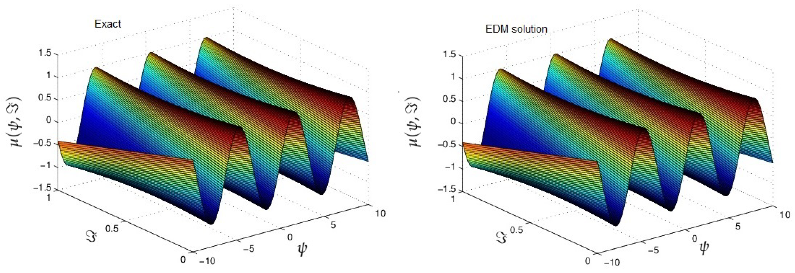
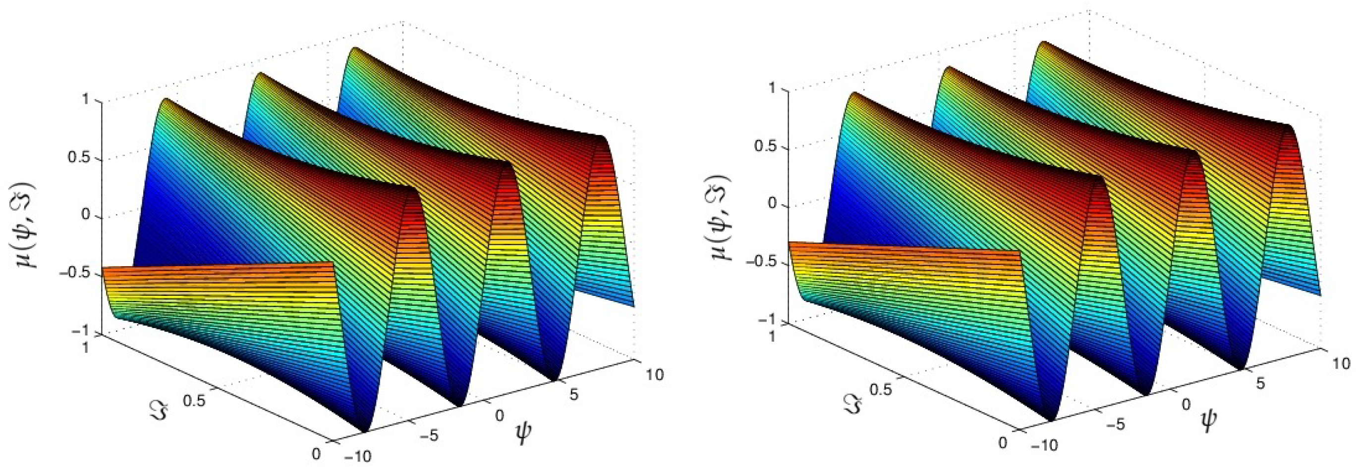
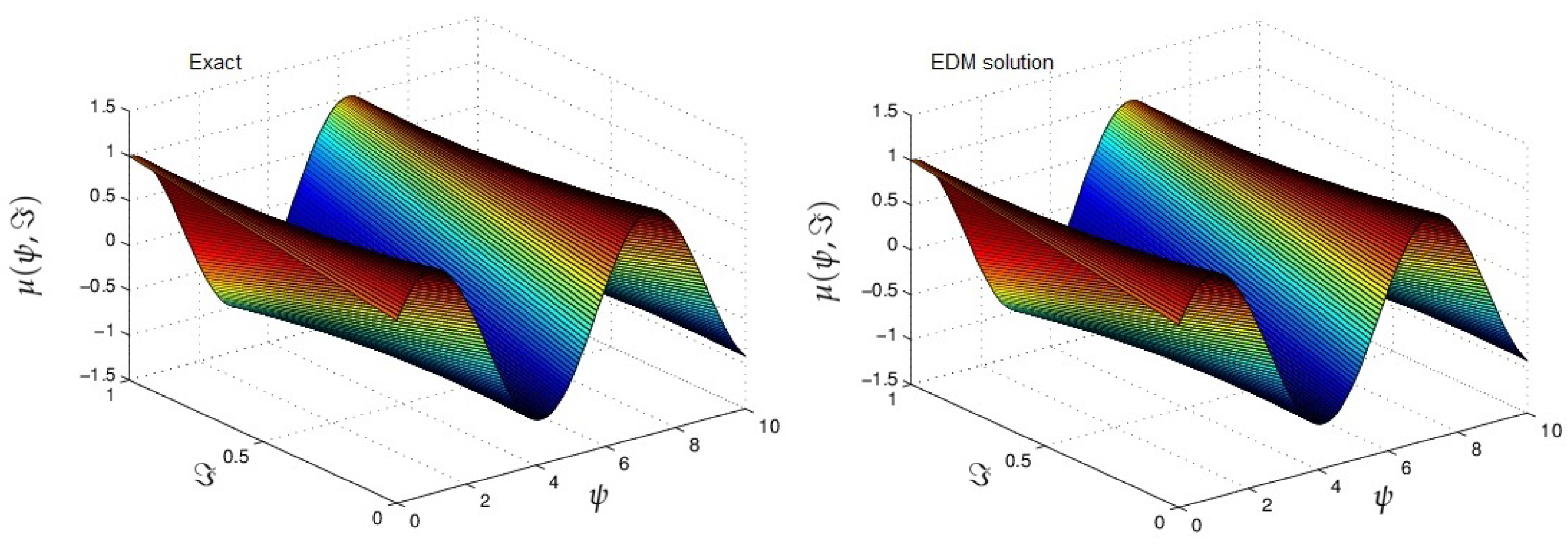
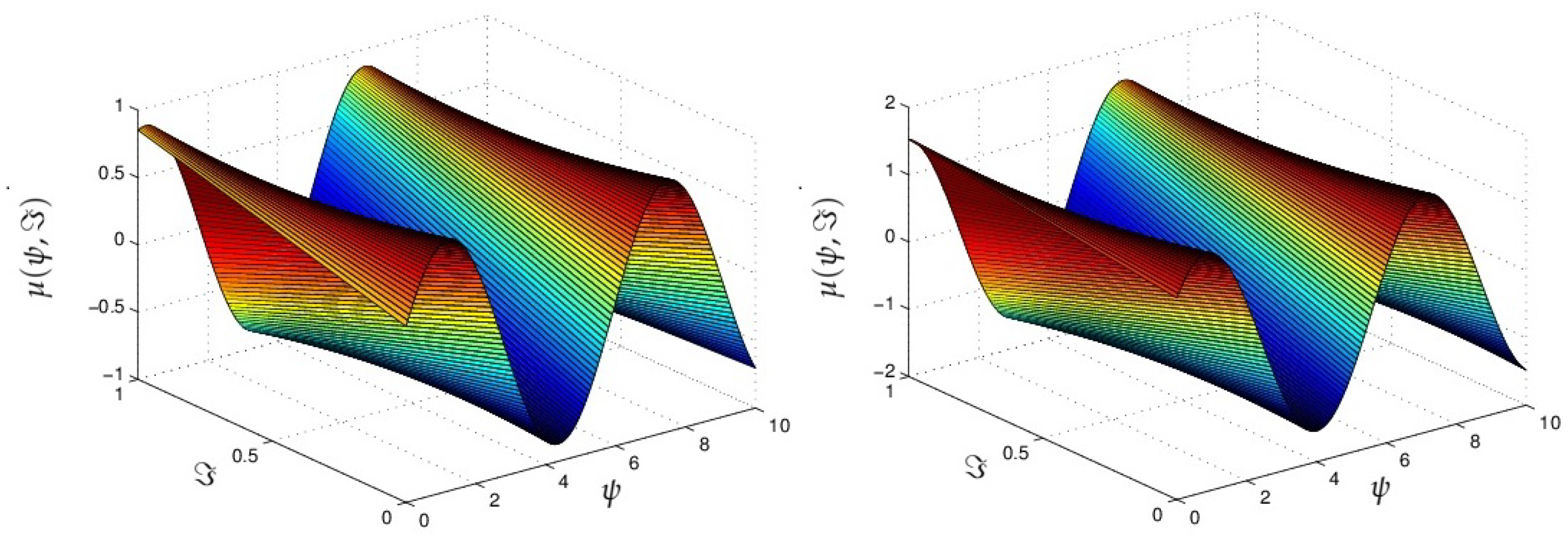
The higher-dimension dispersive partial differential equation is define as,
ϑ μ ϑ + c 3 μ ψ 3 + d 3 μ ϕ 3 + e 3 μ φ 3 = q ( ψ , ϕ , φ , ) , 0 , c , d , e 0 , 0 < ϑ < 1 ,
where the source term is define by q ( ψ , ϕ , φ , ) .
With initial condition is
μ ( ψ , ϕ , φ , 0 ) = k ( ψ , ϕ , φ ) .
Applying Elzaki transformation to Equation (13), we get
E ϑ μ ϑ + E c 3 μ ψ 3 + d 3 μ ϕ 3 + e 3 μ φ 3 = E q ( ψ , ϕ , φ , ) ,
E j = 0 μ ( ψ , ϕ , φ , ) = k ( ψ , ϕ , z ) s 2 + s ϑ E q ( ψ , ϕ , φ , ) s ϑ E c 3 μ ψ 3 + d 3 μ ϕ 3 + e 3 μ φ 3 .
Applying the linearity of the Elzaki transform,
E μ 0 ( ψ , ϕ , φ , ) = μ ( ψ , ϕ , φ , 0 ) s 2 + s ϑ E q ( ψ , ϕ , φ , ) = k ( ψ , ϕ , φ , s ) ,
E μ 1 ( ψ , ϕ , φ , ) = s ϑ E c 3 μ 0 ψ 3 + d 3 μ 0 ϕ 3 + e 3 μ 0 φ 3 .
Generally, we can write
E μ j + 1 ( ψ , ϕ , φ , ) = s ϑ E c 3 μ 1 ψ 3 + d 3 μ 1 ϕ 3 + e 3 μ 1 φ 3 , j 1 .
Applying the inverse Elzaki transform of Equation (16)
μ 0 ( ψ , ϕ , φ , ) = k ( ψ , ϕ , φ , ) ,
μ j + 1 ( ψ , ϕ , φ , ) = E 1 s ϑ E c 3 μ j ψ 3 + d 3 μ j ϕ 3 + e 3 μ j φ 3 .

4. Results

Example 1.
Consider the following fractional-order dispersive KdV equation [29]
ϑ μ ϑ + 2 μ ψ + 3 μ ψ 3 = 0 , > 0 , 0 < ϑ 1 ,
with initial condition
μ ( ψ , 0 ) = sin ψ ,
using Elzaki transformation of (19), we get
E ϑ μ ϑ = E 2 μ ψ + 3 μ ψ 3 ,
1 s ϑ E μ ( ψ , ) s 2 ϑ μ ( ψ , 0 ) = E 2 μ ψ + 3 μ ψ 3 .
Applying inverse Elzaki transform
μ ( ψ , ) = E 1 s 2 μ ( ψ , 0 ) s ϑ E 2 μ ψ + 3 μ ψ 3 ,
μ ( ψ , ) = sin ψ E 1 s ϑ E 2 μ ψ + 3 μ ψ 3 .
Using ADM procedure, we get
j = 0 μ j ( ψ , ) = sin ψ E 1 s ϑ E 2 j = 0 μ j ψ + j = 0 3 μ j ψ 3 ,
μ 0 ( ψ , ) = = sin ψ ,
μ j + 1 ( ψ , ) = E 1 s ϑ E 2 j = 0 μ j ψ + j = 0 3 μ j ψ 3 ,
for j = 0 , 1 , 2 ,
μ 1 ( ψ , ) = E 1 s ϑ E 2 μ 0 ψ + 3 μ 0 ψ 3 = cos ψ ϑ Γ ( ϑ + 1 ) , μ 2 ( ψ , ) = E 1 s ϑ E 2 μ 1 ψ + 3 μ 1 ψ 3 = sin ψ 2 ϑ Γ ( 2 ϑ + 1 ) .
The subsequent terms are
μ 3 ( ψ , ) = E 1 s ϑ E 2 μ 2 ψ + 3 μ 2 ψ 3 = cos ψ 3 ϑ Γ ( 3 ϑ + 1 ) .
The EDM solution for Example 1 is
μ ( ψ , ) = μ 0 ( ψ , ) + μ 1 ( ψ , ) + μ 2 ( ψ , ) + μ 3 ( ψ , ) + .
μ ( ψ , ) = sin ψ cos ψ ϑ Γ ( ϑ + 1 ) sin ψ 2 ϑ Γ ( 2 ϑ + 1 ) + cos ψ 3 ϑ Γ ( 3 ϑ + 1 ) + .
The solution for the series form is provided by
μ ( ψ , ) = sin ψ 1 2 ϑ Γ ( 2 ϑ + 1 ) + 4 ϑ Γ ( 4 ϑ + 1 ) cos ψ ϑ Γ ( ϑ + 1 ) 3 ϑ Γ ( 3 ϑ + 1 ) + 5 ϑ Γ ( 5 ϑ + 1 ) ,
when ϑ = 1 , then EDM solution is
μ ( ψ , ) = sin ( ψ ) .
Figure 1 consists of two plots the exact and EDM results of μ ( ψ , ) of Example 1 at ϑ = 1 . Both the graphs of Figure 1 indicate that the current technique has close contact with the exact result for the given. In Figure 2, two plots are given that represent the approximate result of Example 1 at fractional ϑ = 0.8 and 0.6 , respectively. Show that the solution surfaces of the fractional-order are convergent to the integer-order surface as the fractional-order approaches to the integer-order. It suggests that through the physical phenomena happening in nature, we can model any of the surfaces as desire physically.
Example 2.
Consider the fractional-order dispersive KdV equation [29]
ϑ μ ϑ + 3 μ ψ 3 + 3 μ ϕ 3 = 0 , > 0 , 0 < ϑ 1 ,
the initial condition is
μ ( ψ , ϕ , 0 ) = cos ( ψ + ϕ ) .
Applying Elzaki transformation of (26), we get
E ϑ μ ϑ = E 3 μ ψ 3 + 3 μ ϕ 3 ,
1 s ϑ E μ ( ψ , ϕ , ) s 2 ϑ μ ( ψ , ϕ , 0 ) = E 3 μ ψ 3 + 3 μ ϕ 3 .
Using inverse Elzaki transformation,
μ ( ψ , ϕ , ) = E 1 s 2 μ ( ψ , ϕ , 0 ) s ϑ E 3 μ ψ 3 + 3 μ ϕ 3 ,
μ ( ψ , ϕ , ) = cos ( ψ + ϕ ) E 1 s ϑ E 3 μ ψ 3 + 3 μ ϕ 3 .
Implemented the Adomian decomposition technique, we have
j = 0 μ j ( ψ , ϕ , ) = cos ( ψ + ϕ ) E 1 s ϑ E j = 0 3 μ j ψ 3 + j = 0 3 μ j ϕ 3 ,
μ 0 ( ψ , ϕ , ) = cos ( ψ + ϕ ) ,
μ j + 1 ( ψ , ϕ , ) = E 1 s ϑ E j = 0 3 μ j ψ 3 + j = 0 3 μ j ϕ 3 ,
for j = 0 , 1 , 2 , . .
μ 1 ( ψ , ϕ , ) = E 1 s ϑ E 3 μ 0 ψ 3 + 3 μ 0 ϕ 3 = 2 sin ( ψ + ϕ ) ϑ Γ ( ϑ + 1 ) , μ 2 ( ψ , ϕ , ) = E 1 s ϑ E 3 μ 1 ψ 3 + 3 μ 1 ϕ 3 = 4 cos ( ψ + ϕ ) 2 ϑ Γ ( 2 ϑ + 1 ) .
The subsequent terms are
μ 3 ( ψ , ϕ , ) = E 1 s ϑ E 3 μ 2 3 ψ + 3 μ 2 ϕ 3 = 8 sin ( ψ + ϕ ) 3 ϑ Γ ( 3 ϑ + 1 ) .
The EDM solution for Example 2 is
μ ( ψ , ϕ , ) = μ 0 ( ψ , ϕ , ) + μ 1 ( ψ , ϕ , ) + μ 2 ( ψ , ϕ , ) + μ 3 ( ψ , ϕ , ) , ,
μ ( ψ , ϕ , ) = cos ( ψ + ϕ ) 2 sin ( ψ + ϕ ) ϑ Γ ( ϑ + 1 ) 4 cos ( ψ + ϕ ) 2 ϑ Γ ( 2 ϑ + 1 ) + 8 sin ( ψ + ϕ ) 3 ϑ Γ ( 3 ϑ + 1 ) + ,
The series form solution is given by
μ ( ψ , ϕ , ) = cos ( ψ + ϕ ) 1 4 2 ϑ Γ ( 2 ϑ + 1 ) + 16 2 ϑ Γ ( 2 ϑ + 1 ) sin ( ψ + ϕ ) 2 ϑ Γ ( ϑ + 1 ) 8 3 ϑ Γ ( 3 ϑ + 1 ) + 32 5 ϑ Γ ( 5 ϑ + 1 ) ,
when ϑ = 1 , then EDM solution is
μ ( ψ , ϕ , ) = cos ( ψ + ϕ + 2 ) .
Figure 3 consists of two plots the exact and EDM results of μ ( ψ , ) of Example 2 at ϑ = 1 . Both the graphs of Figure 3 indicate that the current technique has close contact with the exact result for the given. In Figure 4, two plots are given, that represents the approximate result of Example 2 at fractional ϑ = 0.8 and 0.6 , respectively. Figure 4 shows that the solution surfaces of the fractional-order are convergent to the integer-order surface as the fractional-order approaches to the integer-order. It suggests that through the physical phenomena happening in nature, we can model any of the surfaces as desire physically.
Example 3.
Consider the fractional-order nonhomogeneous dispersive KdV equation [29]
ϑ μ ϑ + 3 μ ψ 3 = sin π ψ sin π 3 cos π ψ cos , 0 < ϑ 1 ,
with initial condition
μ ( ψ , 0 ) = sin π ψ ,
using Elzaki transformation of (33), we get
E ϑ μ ϑ = E sin π ψ sin π 3 cos π ψ cos E 3 μ ψ 3 ,
1 s ϑ E μ ( ψ , ) s 2 ϑ μ ( ψ , 0 ) = E sin π ψ sin π 3 cos π ψ cos E 3 μ ψ 3 .
Applying inverse Elzaki transform
μ ( ψ , ) = E 1 s 2 μ ( ψ , 0 ) + s ϑ E sin π ψ sin π 3 cos π ψ cos s ϑ E 3 μ ψ 3 ,
μ ( ψ , ) = E 1 s 2 sin π ψ + E 1 s ϑ E sin π ψ sin π 3 cos π ψ cos E 1 s ϑ E 3 μ ψ 3 .
Implemented the Adomian decomposition technique, we have
j = 0 μ j ( ψ , ) = E 1 s 2 sin π ψ + E 1 s ϑ E sin π ψ 3 3 ! + 5 5 ! 7 7 ! + 9 9 ! + E 1 s ϑ E π 3 cos π ψ 1 2 2 ! + 4 4 ! 6 6 ! + 8 8 ! E 1 s ϑ E j = 0 3 μ j ψ 3 ,
μ 0 ( ψ , ) = sin π ψ sin π ψ ϑ + 1 Γ ( ϑ + 2 ) ϑ + 3 Γ ( ϑ + 4 ) + ϑ + 5 Γ ( ϑ + 6 ) ϑ + 7 Γ ( ϑ + 8 ) + ϑ + 9 Γ ( ϑ + 10 ) π 3 cos π ψ ϑ Γ ( ϑ + 1 ) ϑ + 2 Γ ( ϑ + 3 ) + ϑ + 4 Γ ( ϑ + 5 ) ϑ + 6 Γ ( ϑ + 7 ) + ϑ + 8 Γ ( ϑ + 9 ) ,
μ j + 1 ( ψ , ) = E 1 s ϑ E j = 0 3 μ j ψ 3 ,
for j = 0 , 1 , 2 ,
μ 1 ( ψ , ) = E 1 s ϑ E 3 μ 0 ψ 3 , μ 1 ( ψ , ) = π 3 cos π ψ ϑ Γ ( ϑ + 1 ) π 3 cos π ψ 2 ϑ + 1 Γ ( 2 ϑ + 2 ) 2 ϑ + 3 Γ ( 2 ϑ + 4 ) + 2 ϑ + 5 Γ ( 2 ϑ + 6 ) 2 ϑ + 7 Γ ( 2 ϑ + 8 ) + 2 ϑ + 9 Γ ( 2 ϑ + 10 ) + π 6 sin π ψ 2 ϑ Γ ( 2 ϑ + 1 ) 2 ϑ + 2 Γ ( 2 ϑ + 3 ) + 2 ϑ + 4 Γ ( 2 ϑ + 5 ) 2 ϑ + 6 Γ ( 2 ϑ + 7 ) + 2 ϑ + 8 Γ ( 2 ϑ + 9 ) , μ 2 ( ψ , ) = E 1 s ϑ E 3 μ 1 ψ 3 , μ 2 ( ψ , ) = π 6 sin π ψ 2 ϑ Γ ( 2 ϑ + 1 ) + π 6 sin π ψ 3 ϑ + 1 Γ ( 3 ϑ + 2 ) 3 ϑ + 3 Γ ( 3 ϑ + 4 ) + 3 ϑ + 5 Γ ( 3 ϑ + 6 ) 3 ϑ + 7 Γ ( 3 ϑ + 8 ) + 3 ϑ + 9 Γ ( 3 ϑ + 10 ) + π 9 cos π ψ 3 ϑ Γ ( 3 ϑ + 1 ) 3 ϑ + 2 Γ ( 3 ϑ + 3 ) + 3 ϑ + 4 Γ ( 3 ϑ + 5 ) 3 ϑ + 6 Γ ( 3 ϑ + 7 ) + 3 ϑ + 8 Γ ( 3 ϑ + 9 ) ,
The EDM solution for Example 3 is
μ ( ψ , ) = μ 0 ( ψ , ) + μ 1 ( ψ , ) + μ 2 ( ψ , ) + μ 3 ( ψ , ) + ,
μ ( ψ , ) = sin π ψ sin π ψ ϑ + 1 Γ ( ϑ + 2 ) ϑ + 3 Γ ( ϑ + 4 ) + ϑ + 5 Γ ( ϑ + 6 ) ϑ + 7 Γ ( ϑ + 8 ) + ϑ + 9 Γ ( ϑ + 10 ) π 3 cos π ψ ϑ Γ ( ϑ + 1 ) ϑ + 2 Γ ( ϑ + 3 ) + ϑ + 4 Γ ( ϑ + 5 ) ϑ + 6 Γ ( ϑ + 7 ) + ϑ + 8 Γ ( ϑ + 9 ) + π 3 cos π ψ ϑ Γ ( ϑ + 1 ) π 3 cos π ψ 2 ϑ + 1 Γ ( 2 ϑ + 2 ) 2 ϑ + 3 Γ ( 2 ϑ + 4 ) + 2 ϑ + 5 Γ ( 2 ϑ + 6 ) 2 ϑ + 7 Γ ( 2 ϑ + 8 ) + 2 ϑ + 9 Γ ( 2 ϑ + 10 ) + π 6 sin π ψ 2 ϑ Γ ( 2 ϑ + 1 ) 2 ϑ + 2 Γ ( 2 ϑ + 3 ) + 2 ϑ + 4 Γ ( 2 ϑ + 5 ) 2 ϑ + 6 Γ ( 2 ϑ + 7 ) + 2 ϑ + 8 Γ ( 2 ϑ + 9 ) π 6 sin π ψ 2 ϑ Γ ( 2 ϑ + 1 ) + π 6 sin π ψ 3 ϑ + 1 Γ ( 3 ϑ + 2 ) 3 ϑ + 3 Γ ( 3 ϑ + 4 ) + 3 ϑ + 5 Γ ( 3 ϑ + 6 ) 3 ϑ + 7 Γ ( 3 ϑ + 8 ) + 3 ϑ + 9 Γ ( 3 ϑ + 10 ) + π 9 cos π ψ 3 ϑ Γ ( 3 ϑ + 1 ) 3 ϑ + 2 Γ ( 3 ϑ + 3 ) + 3 ϑ + 4 Γ ( 3 ϑ + 5 ) 3 ϑ + 6 Γ ( 3 ϑ + 7 ) + 3 ϑ + 8 Γ ( 3 ϑ + 9 ) +
when ϑ = 1 , then EDM solution is
μ ( ψ , ) = sin π ψ cos .
Figure 5 consits of two plots the exact and EDM results of μ ( ψ , ) of Example 3 at ϑ = 1 . Both the graphs of Figure 5 indicate that the current technique has close contact with the exact result for the given. In Figure 6, two plots are given that represents the approximate result of Example 3 at fractional ϑ = 0.8 and 0.6 , respectively. Figure 6 shows that the solution surfaces of the fractional-order are convergent to the integer-order surface as the fractional-order approaches to the integer-order. It suggests that through the physical phenomena happening in nature, we can model any of the surfaces as desire physically.
Example 4.
Consider the fractional-order three dimensional nonhomogeneous dispersive KdV equation [29]
ϑ μ ϑ + 3 μ ψ 3 + 1 8 3 μ ϕ 3 + 1 27 3 μ φ 3 = sin ( ψ + 2 ϕ + 3 φ ) cos + sin ( ψ + 2 ϕ + 3 φ ) cos , > 0 , 0 < ϑ 1 ,
the initial condition is
μ ( ψ , ϕ , φ , 0 ) = 0 ,
using Elzaki transform of (38), we get
E ϑ μ ϑ = E sin ( ψ + 2 ϕ + 3 φ ) cos E 3 cos ( ψ + 2 ϕ + 3 φ ) sin E 3 μ ψ 3 + 1 8 3 μ ϕ 3 + 1 27 3 μ φ 3 ,
1 s ϑ E μ ( ψ , ϕ , φ , ) s 2 ϑ μ ( ψ , ϕ , φ , 0 ) = E sin ( ψ + 2 ϕ + 3 φ ) cos E 3 cos ( ψ + 2 ϕ + 3 φ ) sin E 3 μ ψ 3 + 1 8 3 μ ϕ 3 + 1 27 3 μ φ 3 .
Applying inverse Elzaki transform
μ ( ψ , ϕ , φ , ) = E 1 s 2 μ ( ψ , ϕ , φ , 0 ) + s ϑ E sin ( ψ + 2 ϕ + 3 φ ) cos + E 1 s ϑ E 3 cos ( ψ + 2 ϕ + 3 φ ) sin E 1 s ϑ E 3 μ ψ 3 + 1 8 3 μ ϕ 3 + 1 27 3 μ φ 3 ,
μ 0 ( ψ , ϕ , φ , ) = E 1 s ϑ E sin ( ψ + 2 ϕ + 3 φ ) 1 2 2 ! + 4 4 ! 6 6 ! + 8 8 ! .
Implementing the Adomian decomposition technique, we have
j = 0 μ j ( ψ , ϕ , ) = E 1 s ϑ E 3 cos ( ψ + 2 ϕ + 3 φ ) 3 3 ! + 5 5 ! 7 7 ! + 9 9 ! E 1 s ϑ E j = 0 3 μ j ψ 3 + 1 8 j = 0 3 μ j ϕ 3 + 1 27 j = 0 3 μ j φ 3 ,
μ 0 ( ψ , ϕ , φ , ) = sin ( ψ + 2 ϕ + 3 φ ) ϑ Γ ( ϑ + 1 ) ϑ + 2 Γ ( ϑ + 3 ) + ϑ + 4 Γ ( ϑ + 5 ) ϑ + 6 Γ ( ϑ + 7 ) + ϑ + 8 Γ ( ϑ + 9 ) ,
μ 1 ( ψ , ϕ , φ , ) = E 1 s ϑ E 3 cos ( ψ + 2 ϕ + 3 φ ) 3 3 ! + 5 5 ! 7 7 ! + 9 9 ! E 1 s ϑ E 3 μ 0 ψ 3 + 1 8 3 μ 0 ϕ 3 + 1 27 3 μ 0 φ 3 ,
μ j + 1 ( ψ , ϕ , φ , ) = E 1 s ϑ E j = 0 3 μ j ψ 3 + 1 8 j = 0 3 μ j ϕ 3 + 1 27 j = 0 3 μ j φ 3 ,
for j = 0 , 1 , 2 ,
μ 1 ( ψ , ϕ , φ , ) = 0 , μ j + 1 ( ψ , ϕ , φ , ) = 0 .
This readily yields the exact solution
μ ( ψ , ϕ , φ , ) = sin ( ψ + 2 ϕ + 3 φ ) ϑ Γ ( ϑ + 1 ) ϑ + 2 Γ ( ϑ + 3 ) + ϑ + 4 Γ ( ϑ + 5 ) ϑ + 6 Γ ( ϑ + 7 ) + ϑ + 8 Γ ( ϑ + 9 ) ,
when ϑ = 1 , then EDM solution is
μ ( ψ , ϕ , φ , ) = sin ( ψ + 2 ϕ + 3 φ ) sin .
Figure 7 consists of two plots the exact and EDM results of μ ( ψ , ) of Example 4 at ϑ = 1 . Both the graphs of Figure 7 indicate that the current technique has close contact with the exact result for the given. In Figure 8, two plots are given that represent the approximate result of Example 4 at fractional ϑ = 0.8 and 0.6 , respectively. Figure 8 shows that the solution surfaces of the fractional-order are convergent to the integer-order surface as the fractional-order approaches to the integer-order. It suggests that through the physical phenomena happening in nature, we can model any of the surfaces as desire physically.

5. Conclusions

In this paper, the Elzaki decomposition method is implemented to obtain fractional-order multi-dimensional dispersive partial differential equations. The technique gives series form solutions that converge very quickly in actual solutions. It is predicted that the achieved results in this article will be helpful for further analysis of the complicated linear and nonlinear physical problems. The calculations of these techniques are very straightforward and simple. Thus, we deduce that this technique can be implemented to solve other fractional-order partial differential equations.

Author Contributions

The authors declare that this study was accomplished in collaboration with the same responsibility. All authors have read and agreed to the published version of the manuscript.

Funding

This research received no external funding.

Institutional Review Board Statement

Not applicable.

Informed Consent Statement

Not applicable.

Data Availability Statement

The numerical data used to support the findings of this study are included within the article.

Acknowledgments

This research was supported by Basic Science Research Program through the National Research Foundation of Korea (NRF) funded by the Ministry of Education (No. 2017R1D1A1B05030422).

Conflicts of Interest

The authors declare no conflict of interest.

References

  1. Miller, K.S.; Ross, B. An Introduction to Fractional Calculus and Fractional Differential Equations; Wiley: New York, NY, USA, 1993. [Google Scholar]
  2. Kilbas, A.A.; Srivastava, H.M.; Trujillo, J.J. Theory and Applications of Fractional Differential Equations; Elsevier: Amsterdam, The Netherlands, 2006. [Google Scholar]
  3. Podlubny, I. Fractional Differential Equations; Academic Press: New York, NY, USA, 1999. [Google Scholar]
  4. Drapaca, C.S.; Sivaloganathan, S. A fractional model of continuum mechanics. J. Elast. 2012, 107, 105–123. [Google Scholar] [CrossRef]
  5. Deshpande, A.; Daftardar-Gejji, V. Chaos in discrete fractional difference equations. Pramana 2016, 87, 1–10. [Google Scholar] [CrossRef]
  6. Fang, L.; Liu, J.; Ju, S.; Zheng, F.; Dong, W.; Shen, M. Experimental and theoretical evidence of enhanced ferromagnetism in sonochemical synthesized BiFeO3 nanoparticles. Appl. Phys. Lett. 2010, 97, 242501. [Google Scholar] [CrossRef]
  7. Shah, N.A.; Dassios, I.; Chung, J.D. Numerical Investigation of Time-Fractional Equivalent Width Equations that Describe Hydromagnetic Waves. Symmetry 2021, 13, 418. [Google Scholar] [CrossRef]
  8. Goswami, A.; Singh, J.; Kumar, D. Numerical simulation of fifth order Kdv equations occurring in magneto-acoustic waves. Ain Shams Eng. J. 2017, 9, 2265–2273. [Google Scholar] [CrossRef]
  9. Steudel, H.; Drazin, P.G.; Johnson, R.S. Solitons: An Introduction, 2nd ed.; Cambridge Texts in Applied Mathematics; Cambridge University Press: Cambridge, UK, 1989. [Google Scholar]
  10. Djidjeli, K.; Price, W.G.; Twizell, E.H.; Wang, Y. Numerical methods for the solution of the third-and fifth-order dispersive Korteweg-de Vries equations. J. Comput. Appl. Math. 1995, 58, 307–336. [Google Scholar] [CrossRef] [Green Version]
  11. Zahran, M.A.; El-Shewy, E.K. Contribution of Higher-Order Dispersion to Nonlinear Electron-Acoustic Solitary Waves in a Relativistic Electron Beam Plasma System. Phys. Scr. 2007, 6, 803. [Google Scholar] [CrossRef]
  12. Seadawy, A.R. New exact solutions for the KdV equation with higher order nonlinearity by using the variational method. Comput. Math. Appl. 2011, 62, 3741–3755. [Google Scholar] [CrossRef] [Green Version]
  13. Shi, Y.; Xu, B.; Guo, Y. Numerical solution of Korteweg-de Vries-Burgers equation by the compact-type CIP method. Adv. Differ. Equ. 2015, 2015, 353. [Google Scholar] [CrossRef] [Green Version]
  14. Yavuz, M.; Ãzdemir, N. European vanilla option pricing model of fractional order without singular kernel. Fractal Fract. 2018, 2, 3. [Google Scholar] [CrossRef] [Green Version]
  15. Thabet, H.; Kendre, S.; Chalishajar, D. New analytical technique for solving a system of nonlinear fractional partial differential equations. Mathematics 2017, 5, 47. [Google Scholar] [CrossRef] [Green Version]
  16. Yepez-Martinez, H.; Gomez-Aguilar, F.; Sosa, I.O.; Reyes, J.M.; Torres-Jimenez, J. The Feng’s first integral method applied to the nonlinear mKdV space-time fractional partial differential equation. Rev. Mex. Fis. 2016, 62, 310–316. [Google Scholar]
  17. Prakash, A.; Kumar, M. Numerical method for fractional dispersive partial differential equations. Commun. Numer. Anal. 2017, 1, 1–18. [Google Scholar] [CrossRef] [Green Version]
  18. Kocak, H.; Pinar, Z. On solutions of the fifth-order dispersive equations with porous medium type non-linearity. Waves Random Complex Media 2018, 28, 516–522. [Google Scholar] [CrossRef]
  19. Kanth, A.R.; Aruna, K. Solution of fractional third-order dispersive partial differential equations. Egypt. J. Basic Appl. Sci. 2015, 2, 190–199. [Google Scholar]
  20. Sultana, T.; Khan, A.; Khandelwal, P. A new non-polynomial spline method for solution of linear and non-linear third order dispersive equations. Adv. Differ. Equ. 2018, 2018, 316. [Google Scholar] [CrossRef]
  21. Pandey, R.K.; Mishra, H.K. Homotopy analysis Sumudu transform method for time-fractional third order dispersive partial differential equation. Adv. Comput. Math. 2017, 43, 365–383. [Google Scholar] [CrossRef]
  22. Adomian, G. Solving Frontier Problems of Physics: The Decomposition Method; With a Preface by Yves Cherruault; Fundamental Theories of Physicss; Springer Science & Business Media: Berlin/Heidelberg, Germany, 1994; Volume 60. [Google Scholar]
  23. Elzaki, T.M. The new integral transform Elzaki transform. Glob. J. Pure Appl. Math. 2011, 7, 57–64. [Google Scholar]
  24. Elzaki, T.M. On the connections between Laplace and Elzaki transforms. Adv. Theor. Appl. Math. 2011, 6, 1–11. [Google Scholar]
  25. Elzaki, T.M. On The New Integral Transform “Elzaki Transform” Fundamental Properties Investigations and Applications. Glob. J. Math. Sci. Theory Pract. 2012, 4, 1–13. [Google Scholar]
  26. Jena, R.M.; Chakraverty, S. Solving time-fractional Navier-Stokes equations using homotopy perturbation Elzaki transform. SN Appl. Sci. 2019, 1, 16. [Google Scholar] [CrossRef] [Green Version]
  27. Sedeeg, A.K.H. A coupling Elzaki transform and homotopy perturbation method for solving nonlinear fractional heat-like equations. Am. J. Math. Comput. Model. 2016, 1, 15–20. [Google Scholar]
  28. Neamaty, A.; Agheli, B.; Darzi, R. Applications of homotopy perturbation method and Elzaki transform for solving nonlinear partial differential equations of fractional order. J. Nonlinear Evol. Equ. Appl. 2016, 6, 91–104. [Google Scholar]
  29. Wazwaz, A.M. An analytic study on the third-order dispersive partial differential equations. Appl. Math. Comput. 2003, 142, 511–520. [Google Scholar] [CrossRef]
Figure 1. The graph of Exact and EDM solutions of ϑ = 1 of Example 1.
Symmetry 13 00939 g001
Figure 2. The graphs of different fractional-order ϑ = 0.8 and 0.6 of Example 1.
Symmetry 13 00939 g002
Figure 3. The graph of Exact and EDM solutions of ϑ = 1 of Example 2.
Symmetry 13 00939 g003
Figure 4. The graphs of different fractional-order ϑ = 0.8 and 0.6 of Example 2.
Symmetry 13 00939 g004
Figure 5. The graph of Exact and EDM solutions of ϑ = 1 of Example 3.
Symmetry 13 00939 g005
Figure 6. The graphs of different fractional-order ϑ = 0.8 and 0.6 of Example 3.
Symmetry 13 00939 g006
Figure 7. The graph of Exact and EDM solutions of ϑ = 1 of Example 4.
Symmetry 13 00939 g007
Figure 8. The graphs of different fractional-order ϑ = 0.8 and 0.6 of Example 4.
Symmetry 13 00939 g008
Publisher’s Note: MDPI stays neutral with regard to jurisdictional claims in published maps and institutional affiliations.

