Abstract
Numerical models for the flow of blood and other fluids can be used to design and optimize microfluidic devices computationally and thus to save time and resources needed for production, testing, and redesigning of the physical microfluidic devices. Like biological experiments, computer simulations have their limitations. Data from both the biological and the computational experiments can be processed by machine learning methods to obtain new insights which then can be used for the optimization of the microfluidic devices and also for diagnostic purposes. In this work, we propose a method for identifying red blood cells in flow by their stiffness based on their movement data processed by neural networks. We describe the performed classification experiments and evaluate their accuracy in various modifications of the neural network model. We outline other uses of the model for processing data from video recordings of blood flow. The proposed model and neural network methodology classify healthy and more rigid (diseased) red blood cells with the accuracy of about 99.5% depending on the selected dataset that represents the flow of a suspension of blood cells of various levels of stiffness.
1. Introduction
Research and development in the field of microfluidics have increased significantly in recent years. One of the main focuses has been the study of the behavior of fluids in microfluidic devices as well as the development of technologies for manufacturing such devices of various shapes, sizes, and materials. The inner structure of these devices ranges from simple straight channels with few or no obstacles to complex geometric designs with a very specific use [1].
Testing real prototypes of microfluidic devices for their further improvement is often technologically demanding, expensive, and time-consuming. Numerical models of blood flows offer an alternative approach. One of the main advantages is that the topology of the channel in the numerical model can be easily changed, allowing the evaluation of the behavior of cells in the flow under various conditions. Thus, the functionality of the proposed device can be verified at a much lower cost, and only the devices with optimal design of their inner structure can be manufactured and tested. Cell in Fluid, Biomedical Modeling & Computation Group (CIF) [2] developed a numerical model of RBC immersed in fluid [3]. One of the main research objectives of CIF is the optimization of the inner structure of microfluidic devices designed to capture and sort circulating tumor cells from other solid blood components [4]. These devices can be used for early diagnosis of cancer using only a blood sample. The identification and enumeration of circulating tumor cells can also help to indicate the effectiveness and suitability of the prescribed treatment. Research at CIF also focuses on other topics related to microfluidics, such as the study of red blood cell (RBC) damage occurring when the cells pass through a microfluidic channel, or the investigation of bulk properties of dense cell suspensions in the blood flow [5,6].
Although there are many advantages to using numerical models, they are quite complex and thus require advanced hardware and extensive computational time—especially simulations of blood suspensions with higher hematocrits. Each simulation provides a large amount of output data and, usually, only a small fraction of it is used to evaluate a specific phenomenon. However, the already obtained output data can be processed with suitable statistical methods to gain more information, see [7,8,9]. This motivated us to further investigate and process data from the simulations using various machine learning methods.
We propose three main possible applications of machine learning in the study of blood flow simulations: verification (and possible improvement) of the previously used numerical models, design of new, faster computational models, and acquisition of further results from simulation data without the performance of new simulation experiments. Machine learning is well suited for analyzing large sets of data, such as the simulation output data. The proposed machine learning models can be also used to process data from video recordings of biological experiments. However, it is more difficult to obtain suitable data from laboratory experiments than from computer simulations for several reasons: most importantly, biomedical studies often include only information relevant to the studied topic, instead of all the information needed for precise computer simulations of these experiments. Furthermore, the presented data are often not only insufficient but also inaccurate due to high technical requirements for a high-quality video recording of the experiment.
The Importance of Red Blood Cells Rigidity Classification
In the diagnosis of various diseases such as sickle cell anaemia, malaria, diabetes, or leukemia, it is important to detect diseased cells in a blood sample, see [10,11]. Diseased RBCs lose their natural elasticity and become more rigid. In the study [12], it was shown that more rigid RBSc infected with malaria are pushed by the healthy RBCs to the edges of the flow. This observation was used to distinguish diseased RBCs from healthy ones by using a microfluidic device with side outlets. Diseased RBCs behave similarly to leukocytes in blood vessels with a diameter of less than m. RBCs, which are smaller in size and more deformable than leukocytes, migrate to the axial center of the vessel due to the flow rate gradient in the vessels, while the leukocytes are pushed to the walls of the vessel. In this paper, we use a neural network model to address the problem of distinguishing RBCs with other elastic properties and determining the ratio of diseased and healthy RBCs in the blood flow. A sufficiently accurate classification model should not only be able to find diseased cells but also to determine their number in the hematocrit. This makes it possible to diagnose and determine the severity of the disease and then apply the appropriate treatment.
2. Related Work
In recent years, several studies have addressed the problem of classification of blood cells from microscopic images of blood using various machine learning methods. In the [13] study, a convolutional neural network (CNN) model was used to classify eight different shapes of RBCs suffering from sickle cell anaemia from microscopic images of RBCs. The model achieved a success rate of around . Different neural network (NN) models have been used to distinguish between healthy RBCs and malaria-infected RBCs. In one of the most recent studies [14], the CNN model identified infected blood cells with an accuracy of and classified different types of infected cells with an accuracy of . In this paper, we propose a model with a classification accuracy of around .
Linear Model for the Identification of More Rigid Blood Cells
To compare the simulation model with the results of biological experiments, it is necessary to determine their differences—for example, by comparing video recording of blood flow from biological experiments and simulation. We compared how the linear model identifies diseased blood cells using the cell movement dataset (obtained from the simulation outputs) and using a dataset obtained from a video recording of visualization of the same simulation. The outputs from the simulation are three-dimensional geometric data representing the position and shape of the blood cell, and the outputs from the video are a two-dimensional projection of the blood cell onto the selected plane, see Figure 1. In addition to the position of the extremal points, we also use the velocity vector at the blood cell center of the mass. In the 3D model (simulation output), the dataset for each blood cell consists of the vectors of the maximum distance in the direction of the axes, i.e., , , , and the velocity of the blood cell center of mass , , . The fluid flow is in the direction of the x-axis. In the 2D model, which represents a video recording of the experiment, we work with projections onto the plane or the plane. Since we do not work with gravity in the computational simulation model, both projections should be equivalent. This section aims to demonstrate what results can be achieved using the Principal component analysis method, and subsequently the possibilities of their improvement when using neural networks. In the specific case of a dataset with of slightly damaged blood cells, we show how the results differ in the 3D and 2D cases with the linear approach. Then, we show that, although the simulation was symmetric in the direction of the y- and z-axes, the Principal components analysis gives better results when projected on the y-axis than when projected on the z-axis.
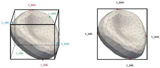
Figure 1.
3D and 2D cuboids obtained from the simulation and from the video.
In the following examination, we used data from simulation experiment Ae20b, which is described in Section 3.1. As an input to the Principal component analysis, we used a matrix of 3D positions of extremal points and center velocities in the direction of all three axes. In the next step, we calculated the projections of these vectors onto the planes and and calculated the distance of the vector and its projection. The average distance between the vectors and their projections serves as a boundary h, by which we distinguish between healthy and diseased blood cells. According to the rigidity of the diseased blood cells and according to the ratio of their number to the number of healthy blood cells, we multiply the value of h by an empirically determined coefficient, in our case, the coefficient is equal to . The use of the Principal component analysis method gives us a good estimate for the effectivity of linear models. The identification of healthy and slightly damaged blood cells, the damage of which is not determinable from their geometric shape, can be made from the variance and mutual ratio of individual vectors connecting the extremal points. For blood cells in the stabilized part of the simulation, the success rate of blood cell identification is determined in Table 1.

Table 1.
Identification success rate for cells from simulation of blood flow.
The simplification of information in the case of the video recording of the simulation causes a reduction in accuracy. We compare the success rate of the identification in the case of simulation (i.e., three-dimensional information about cells) and in the case of video recording (two-dimensional video recording of the same simulation experiment as in Table 1). The results from the video in the case of a projection onto two different planes are in Table 2 and Table 3.
Table 2.
Identification success rate for video of simulation in plane .
Table 3.
Identification success rate for video of simulation in plane .
Although we expected essentially the same success rate for video recordings in the plane and the plane, the results show that simulations recorded from a “side view” have better resolution for identification of diseased blood cells than simulations recorded from the “top view.” This is likely due to statistical differences between the data describing the distribution and slopes of the RBCs in the individual planes. For example, in Figure 2, we see a different distribution of described cuboid side lengths in the y-axis direction and the z-axis direction. For the linear model, these differences are large enough to cause changes in the classifier performance. As we will show below, classification using neural networks is more robust and reduction to a 2D case produces the same and even better results in all directions.
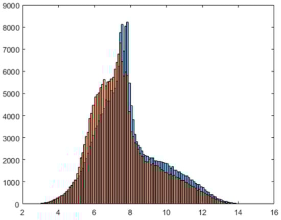
Figure 2.
Distribution of described cuboid lengths in the y-axis direction (blue) and the z-axis direction (orange).
3. Materials and Methods
Our method processes data describing the movement of RBCs in a simulation box. Instead of using a microscopic image of the cell as the input, we use the time sequence of its positions. This is a potential advantage when working with video data from laboratory experiments. Since these videos are often of insufficient quality, it is difficult to obtain an accurate picture of the cell. On the other hand, there are known methods for detection of the rectangular or elliptic area in which the cell is located, which can be used to describe the trajectories of RBCs, see [15,16]. Our goal is to develop a NN model which classifies RBCs by their rigidity, identifying them as healthy or diseased. The input of the model is a time sequence of positions of a given length ℓ (usually, we have ). The total number of positions t for a given cell differs for each simulation experiment, but, in each case, we have , see Table A3. Our model randomly chooses a number i between 1 and , and then takes the sequence of l consecutive positions starting at the i th position. This way, some sequences might enter the model more than once, but it is faster than using all possible sequences of positions.
3.1. Description of Simulation Experiments
The data entering our NN model come from blood flow simulation experiments. These simulations were performed to investigate the effect of various factors, such as the ratio of healthy and diseased cells in the flow, the flow rate, or the elasticity of damaged cells, on the level of margination of diseased blood cells. Margination was formed for suspensions with a majority of healthy cells, and was more apparent in simulations with longer running times. In the used numerical model [17], the control of fluid dynamics is ensured by the lattice-Boltzmann method [18], and the elasticity of the cell membrane is controlled by the spring network model [19]. Fluid and blood cells are connected by the dissipative version of the Immersed Boundary Method (DC-IBM).
The dimensions of the simulation box are m, and the box does not contain any other walls or obstacles. RBCs flow in the direction of the x-axis from left to right, and the channel is periodic in this direction. (This means that, if a cell leaves the simulation box at one end, then it reenters it on the other end.)
The RBC model is discrete, consisting of a triangulation of the RBC surface. The modeled suspension contains 154 RBCs, each with 374 nodes. This represents a hematocrit, which corresponds to the flow of blood in narrow blood vessels. We used data from 13 simulations. Individual simulations differ in the ratio of healthy and diseased RBCs, in the rigidity of diseased RBCs, and the initial location of RBCs. The rigidity of RBC is determined by its elastic parameters. Stretching coefficient has the largest influence on RBC rigidity, thus we determine the rigidity of the RBCs by the value of the stretching coefficient . Figure 3 shows shapes of diseased blood cells depending on the value of the stretching coefficient. In the individual experiments, all diseased RBCs had the same elastic parameters, which we list in Table A1 in the appendix. Similarly, the elastic parameters of healthy RBCs (also shown in Table A1) and their mutual interactions were also the same for all experiments.The parameters of the fluid are listed in Table A2.
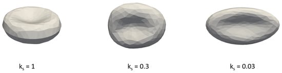
Figure 3.
The elasticity of diseased RBC depending on the value of the stretching coefficient .
Figure 4 shows simulated RBCs in the channel. Gray cells with represent healthy RBCs, while red cells with represent diseased RBCs. Table A3 shows the names of used simulations, and, for each simulation, we list the number of time records for a cell in the corresponding experiment. Some of the simulations are based on the previous ones. (In this case, the name of the new simulation differs from the name of the original simulation only by letter e.) The first letter (or pair of letters) of the name of a simulation indicates the initial location of the cells. The number that follows indicates the proportion of diseased cells in the blood, and the last lower case letter indicates the rigidity of the diseased blood cells. (The letter a indicates the most rigid diseased blood cells (), while the letter c indicates the least rigid diseased blood cells ().)
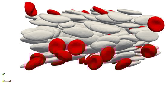
Figure 4.
Cells in the simulation channel during the simulation.
3.2. Dataset and Data Preprocessing
The training and test data come from simulation output files in “.dat” format. We had to crop them appropriately to the shortest distance since, for some simulations, the number of recorded cell positions was not the same. In the classification experiments, we use various simulation data about the cell movement:
- the positions of the cell centers in x, y, and z-directions, giving three data types for each RBC,
- the positions of all six extremal points of cells in each direction x, y, and z (with or without the center of the cell), giving either 18 or 21 data types for each RBC,
- the positions of four extremal points of cells for all 3 coordinate planes , and in all directions (with or without the center of the cell), giving either 12 or 15 data types for each RBC,
- the positions of four extremal points only in the direction of the selected coordinate planes (without the center of the cell) for all 3 coordinate planes , and , giving 8 data types for each RBC.
The last selection of data represents a two-dimensional image of a cell (see Figure 5b), from which we can easily obtain a rectangular or elliptic area in which the cell is located. The same can be done for video recordings of laboratory experiments. A sufficiently accurate model for classifying cells could thus be used to classify them from blood flow video recordings.
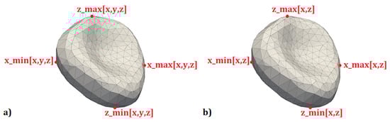
Figure 5.
(a) The extremal points of the cell in the plane in all three directions; (b) the extremal points of the cell in the plane in the direction of the selected axes.
First, we normalized all data with an average of 0 and a variance of 1, individually for each of the 3 to 21 data types used. For a sufficiently large volume of training data, we add augmented data to the training dataset, which we create by adding a slight noise and shifting the original positions. In most experiments, we use 100 augmentations, which means that, for each cell in each time step, we add 100 extra positions shifted in all directions from the original position. The size of the training dataset is
where is the number of augmentations, and is the number of time records of cell movement in the simulation experiment. Recall that, in all experiments, there are 154 cells. For example, the size of a training dataset that uses simulation data containing 700 time records of each cell’s motion, and 100 augmentations, is 10,887,800. The diagram in Figure 6 shows the classification model and dataset preprocessing.
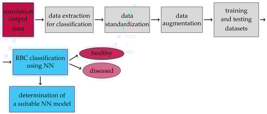
Figure 6.
Flow chart of our proposed model for the classification of healthy and diseased cells in blood flow.
Dataset names are derived from the names of the simulation experiments in Table A3. The name of the simulation experiment whose data were used for training is followed by the name of the simulation experiment whose data were used for testing, separated by an underscore. For example, A20a_Ae20a is the name of a dataset that uses data from the A20a simulation for training and data from the Ae20a simulation for testing.
3.3. Tested Network Architectures for RBC Rigidity Classification
We used 22 different models of neural network architectures, which are derived from the 5 basic models shown in Table 4. Three of these basic networks Conv, ResNet_1 and ResNet_2 are convolutional, and the other two LSTM and GRU are recurrent neural networks. In total, we used 14 different convolution and eight recurrent NN models. Network architectures are shown in Figure 7.
Table 4.
Network architectures.
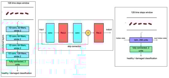
Figure 7.
On the left—convolutional neural network architecture Conv, in the middle—the scheme of the residual block of the network ResNet and on the right—the architecture of the recurrent neural network LSTM.
Since the input data are one-dimensional, all CNN architectures contain only one-dimensional convolution with a kernel of size 3. In the case of residual blocks, we combine two such one-dimensional convolutions. Each convolution layer is followed by a ReLU activation function. For ResNet_1 and ResNet_2, the same types of convolution layers are used, differing only in size. The first number of the convolution layer in Table 4 expresses the size of the kernel and the second number, the number of outputs. In addition, the number of outputs per layer expresses the number in the residual block. The flatten layer arranges the output of the previous layer into a vector, and the fully connected layer has 2 outputs, one representing a healthy and one a diseased cell.
For convolutional networks, we also used the regularization parameter dropout [20]. For the Conv network, dropout follows after the convolution layer (activated by the ReLU function) and, for ResNets architectures, dropout follows after the residual block unless otherwise stated. In Table A4, the dropout values for the 3 basic CNN models are marked, as well as which layers of the respective network followed.
For both recurrent networks, the values of two parameters were changed: the number of neurons and the size of the time window that is the length of the sequence for the learning. A time window of 64 and 128 and a number of neurons of 64 and 256 were used. For dataset A20a_B20a, we trained networks for all combinations of values of these parameters that is 4 LSTM and 4 GRU networks. There were 20 augmentations in these experiments. For the 128 time window, both neuron counts, and both recurrent networks, we repeated the experiments with 100 augmentations.
3.4. Network Training and Hyperparameters
The ADAM training algorithm [21] was used in all experiments. We minimize the loss function:
where are the required values, are the predicted values, and n is the size of the dataset. Model training lasts 100 epochs, unless otherwise stated. A cyclical learning rate [22] with a period of 7 that takes on the following values was used: . The weights were initialized by the Xavier uniform method [23], the bias was set to 0, and the minibatch size was 256 [24]. The parameters used for regularization have the following values: , for the respective values of the cyclical learning rate. The dropout setting is described above.
3.5. Technological and Computational Tools
Models are implemented using PyTorch [25] and trained on the NVIDIA GeForce GTX 1080 Ti graphical processing unit. Source codes are available online in the git repository: https://github.com/katkaj/rbc_classification (accessed on 15 April 2021).
4. Results
More than 100 classification experiments were performed to obtain the most efficient model possible. Network design and input data selection were also optimized (Section 4.1). In the following sections, we compare the accuracy of optimal models concerning the following parameters:
- the selection of extremal points (input data),
- rigidity of diseased RBCs,
- ratio of the healthy and the diseased cells in training and test data,
- margination rate of diseased cells in training data.
These parameters are used as validation criteria of the optimal model(s), and also to find out what differences in training and testing data the model can handle. (That is, to determine when it still achieves sufficient accuracy.) Insufficient accuracy of classification can also indicate shortcomings in the simulation data.
The accuracy of classification on individual (training and test) datasets is expressed in percentage as a weighted average of the accuracy of classification of healthy RBCs and the accuracy of classification of diseased RBCs.
In the Appendix A in Table A5, Table A6 and Table A7, we list the datasets that were used in the experiments for each evaluation.
4.1. Comparison of Model Accuracy with Respect to Input Data Selection and Neural Network Architecture
In Table 5, the accuracy of experiments that uses the positions of cell centers as the input, and experiments that use the positions of cell extremal points is compared. In the latter, we include all experiments in which any type of information about the position of extremal points (listed in Section 3.2) is used. All nine datasets that were used for classification based only on the center of cells were also used for classification based on the extremal points. The list of datasets used in this evaluation, the number of experiments performed, and the neural network architectures used for these datasets are given in Table A5.
Table 5.
An overview of classification experiments and their accuracy with respect to the choice of input data.
From the average testing accuracies given in Table 5, we see that it makes sense to use classification based on the extremal points of cells. Models that used only cells’ center positions were generally unable to classify diseased cells. The most accurate model classified them only with an accuracy of .
4.1.1. Comparison of the Efficiency of Used Neural Network Models
Several neural network architectures were used for classification from cell center positions. In this case, the choice of network architecture did not significantly affect the accuracy of the model.
In the case of classification from -coordinates of all extremal cell points and cell centers, we used five different neural network architectures for one dataset Be20a_Ae20a: Conv_4d001, ResNet_1_4d001, Resnet_2, LSTM and GRU. Conv_4d001 network achieved the best performance, as shown in the graphs in Figure 8. It has reached accuracy already in the 10th epoch. In all other experiments where cell extremal points entered, only this network was used.
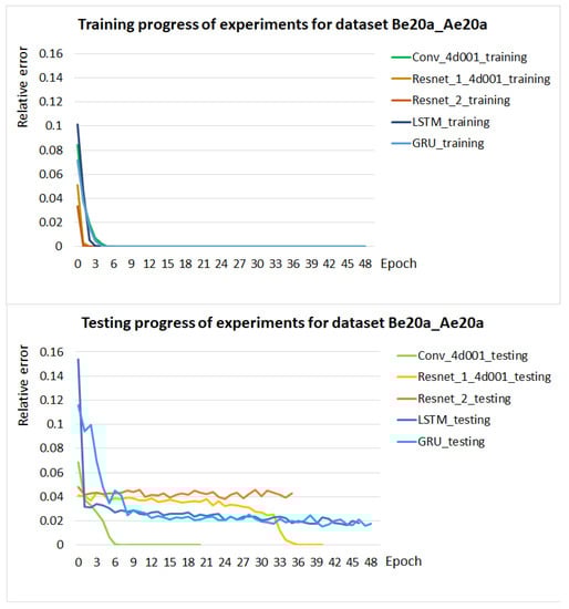
Figure 8.
Training and testing progress of models for five different network architectures during 50 training epochs. The progress of the experiments is shown as the relative error of the accuracy of the experiments in the individual epochs.
4.1.2. Comparison of Model Accuracy with Respect to the Choice of Extremal Points
For the Be20a_Ae20a dataset, the Conv_4d001 network for 11 different selections of extremal points as NN input data was tested. We chose the positions of all six extremal points in all directions (with or without the center of the cell), four extremal points for all three coordinate planes in all directions (with or without the center of the cell) or four extremal points only in the direction of the selected planes (without the center of the cell). All experiments achieved accuracy in both the training and the testing phases.
Furthermore, when selecting four extremal points, we have limited ourselves to the coordinates in which we select the extremal points. From this choice of extremal points, we can obtain the described rectangle of the cell image. The reason for this choice is to detect cells from the video.
For seven different datasets, experiments using all six extremal points in all directions (hereinafter referred to as ) and four extremal points in two directions for all three coordinate planes (hereinafter referred to as , and ) were performed. The overall accuracy of their testing is given in Table 6.
Table 6.
The overall accuracy of the testing model with the Conv_4d001 network architecture with respect to the selection of the training and testing dataset and the choice of input data, and the average of the overall testing accuracy of the given experiments with respect to the selection of the input data.
The differences in the accuracy of the experiments depending on the choice of extremal points are minimal. The use of extremal points in the coordinate planes and was the most advantageous. This result is expected because the blood flows in the direction of the x-axis and therefore the elongation of the elastic blood cell is greatest in this direction.
The graph in Figure 9 compares the test progress of 12 experiments. They use three various datasets and four extremal point selections as in Table 6.
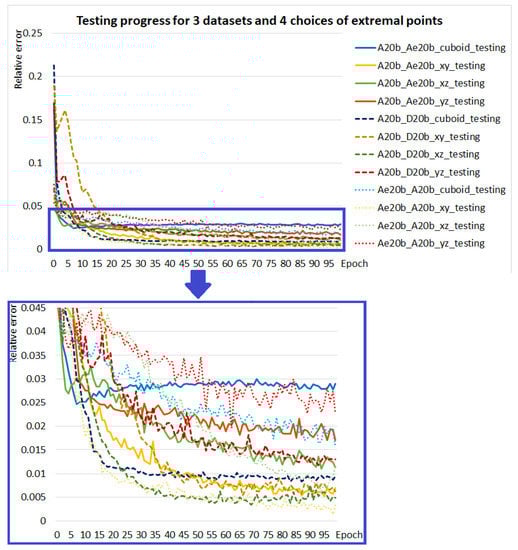
Figure 9.
Testing progress of models for datasets: A20b_Ae20b (solid line), A20b_D20b (dashed line), and Ae20b_A20b (dotted line) and for each of them for input selections: (blue curves), (yellow curves), (green curves) and (red curves). The bottom graph is an enlargement of the selected area of the top graph.
4.2. Comparison of the Accuracy of the Model with Respect to the Rigidity of Diseased Cells
In this and the following sections, only relevant experiments are selected to evaluate the accuracy of the models. We select them for optimal models, i.e., for models with network architecture Conv_4d001 and with input data of cuboid, , , or choices of extremal points. If necessary, the selection of experiments is specified in each section.
As mentioned above, we used three types of rigid (diseased) cells, which vary in the simulations by different settings of the stretching coefficient of the RBC. In Table 7, the average accuracy of experiments with respect to the elasticity of diseased blood cells in a dataset is compared. For the dataset Be20a_Ae20a, which uses the most rigid RBC with the value of the stretching coefficient , 12 experiments were performed (which turned out equally well with accuracy in training and testing) and for other datasets, at most four experiments were performed. In this comparison, only four experiments for dataset Be20a_Ae20a are included. In comparison, there are all experiments from Section 4.1.2 and two experiments with the dataset A20c_Ae20c.
Table 7.
Overview of classification experiments and their accuracy with respect to the rigidity of diseased cells.
From the results in Table 7, we see that, for and , the models achieve comparably accurate results. For the most rigid cells , the classification was accurate for some datasets. For , the accuracy was never ; however, the worst testing accuracy was . For the least rigid cells , the network learned to classify diseased cells, but could not recognize them in the test dataset. These cells are more elastic and thus more similar to healthy RBCs. The data from these simulations did not show a characteristic feature for damaged cells—margination. Therefore, it is not surprising that the network cannot distinguish them so well.
4.3. Comparison of Model Accuracy with Respect to Different Ratios of Healthy and Diseased Cells in Training and Test Data
For the most rigid type of diseased blood cells, we have datasets with , and of diseased RBCs. We performed six experiments where the network was trained and tested on datasets with different ratios of healthy and diseased cells. We used three datasets, each with a different ratio of healthy and diseased cells, which we alternated for training and testing, see Table A6. Networks were trained using the x, y coordinates of the positions of extremal points of cells in the plane. For all the experiments, the trained network was able to very accurately classify the RBCs on the test set. The average accuracy of total testing is , with the worst result of total testing being for a network that trained on data with diseased blood cells and tested on data with diseased blood cells. Based on these results, we can say that the different ratio of healthy and diseased blood cells in the training and testing data does not affect the accuracy of the model. A comparison of the performed experiments is in the graphs in Figure 10. Note that we did not train up to 100 epochs in experiments that achieved accuracy on the test set.
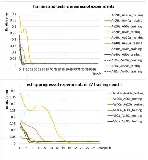
Figure 10.
The graph in the figure above shows the training (dashed line) and testing (solid line) progress of six experiments with different ratios of healthy and diseased cells in the training and test dataset. The graph in the figure below compares the test progress of these experiments in 27 learning epochs.
4.4. Comparison of the Accuracy of the Model with Respect to the Margination of Diseased Cells in Training Data
For three datasets, the network was trained on data from the (beginning) of the simulation, where margination of diseased blood cells did not occur or was minimal, and we tested it on data that was sufficiently marginalized. An overview of datasets is in Table A7. These experiments aim to determine whether the model can distinguish cell damage without being able to learn their characteristic behavior, i.e., margination. For each dataset, four experiments were performed with extremal point choices as shown in Table 6. The average overall accuracy of testing is , which is approximately less than for four selected datasets in which training data are marginalized, see Table 8. For comparison, experiments with marginalized training data were selected, where the networks trained on the same choice of positions of cell extremal points as for datasets with training data without margination. The classification is the most accurate for the input where the positions of or extremal point are used (see Section 4.1.2). The average overall testing accuracy is for training data from experiments without margination and for training data from experiments with margination. The difference between them has narrowed to . From these results, we conclude that information about margination in training data does not significantly affect the accuracy of the classification of healthy and diseased blood cells.
Table 8.
Accuracy of experiments with respect to margination of diseased cells in a training dataset.
4.5. Discussion
From the experiments performed, the model of convolutional neural network with one-dimensional convolutional kernels achieves the best results using the x and y coordinates of cell extremal point positions in the plane or the x and z coordinates of cell extremal point positions in the plane, with blood flowing in the direction of the x-axis. Thus, the network has cell position information in two dimensions. As a result, this model could have good results in classifying healthy and diseased cells from video recordings of laboratory experiments where areas in which the cells are located are detected.
The more rigid the damaged blood cells in the dataset are, the more accurately the model classifies them. For diseased blood cells with values of the stretching coefficient, , the accuracy of classification was on average , while the worst performing experiment with optimal choice of model parameters had an accuracy of . On data with less rigid damaged blood cells with a value of , the model learned to classify diseased cells but could not recognize them in the test data. On the other hand, the data from these simulations did not show the margination that is characteristic of rigid cells.
The experiments also show that the trained network classifies blood cells on datasets with a different ratio of diseased cells with sufficient accuracy (on average with accuracy from the performed experiments at and representation of diseased cells in the hematocrit). The results of experiments where the network is trained on data that are not marginalized suggest that information about margination does not significantly affect the accuracy of the classification of healthy and diseased blood cells.
Furthermore, the models are sufficiently accurate if they have information about the extremal points of the cells and, conversely, if they only have information about the positions of the center of the cell, they usually are unable to distinguish diseased cells sufficiently. These findings support the hypothesis that the model distinguishes blood cells based on their shape rather than their trajectory.
The average overall accuracy of testing experiments with the optimal model and datasets with the stretching coefficient of at least is , where all values are from the interval .
5. Conclusions
The motivation for this work was the applications of computational methods to experimental blood flow data for diagnostic purposes. We show the main methods of numerical modeling of microfluidic devices that are used for the identification and separation of diseased cell from blood flow.
The simulation model and its parameters can be correctly set only when the flow from the biological and the computational experiment can be compared. Since any simulation model is only an approximation of a real biological experiment, it is not possible to compare individual cells, but it is necessary to compare the bulk, statistical properties and behavior of the cells.
Linear models can describe some of the characteristics of the blood flow and they can be used to compare these characteristics with statistics obtained from the simulation model. However, there is usually only 2D video recording or photo available for real biological experiment processing.
This leads to important questions. How similar is the video recording of the experiment compared to the real experiment? How much information about the experiment can be obtained from 2D recording? How much information is lost and how does it affect diagnostic results?
The answers to the questions about the statistical comparison of experiments were developed in the following works [7,8,9]. Questions about the application of computational methods for diagnostic purposes are covered in this paper.
Neural networks were used for the identification of diseased cells. The models classify RBCs based on the time sequences of their positions. In addition, 116 experiments were performed with various neural network architectures. We used different ratios of the diseased and healthy blood cells, different types of diseased cells, and different ranges of input information about individual cells. The result is a complex comparison of the effectivity of the neural network use for this classification problem. The tables show how individual settings influence the overall diagnostic success. These results can be interpreted as the rate of difference in solving this problem in a situation where we have data from video recording or more complex data from the simulation.
Further research can ponder the effectiveness of the neural network in cases when the input dataset is damaged. The question is if the neural network will be able to learn future behavior of the simulation even in the cases when it will receive no information about this behavior. We focused on diagnostics of the disease that manifest with more rigid RBC. If we could obtain information about the typical manifestation of other diseases in blood cell behavior, we could focus on their diagnostics. However, neural networks allow for diagnostics of diseases of which we have no prior knowledge of how they manifest in blood cell behavior. Then, it will become a problem of explainability if we will be able to not only diagnose these diseases but also recognize them on a cellular level.
Author Contributions
Conceptualization, K.B. (Katarína Bachratá), H.B. and M.C.; methodology, M.C. and K.B. (Katarína Buzáková); software, M.C. and K.B. (Katarína Buzáková); validation, M.C., K.B. (Katarína Buzáková) and M.S.; formal analysis, K.B. (Katarína Buzáková); investigation, K.B. (Katarína Buzáková) and M.S.; resources, M.S. and M.C.; data curation, M.S. and M.C.; writing—original draft preparation, K.B. (Katarína Buzáková) and K.B. (Katarína Bachratá); writing—review and editing, H.B., K.B. (Katarína Bachratá), A.B., M.C. and M.S.; visualization, K.B. (Katarína Buzáková); supervision, K.B. (Katarína Bachratá); project administration, K.B. (Katarína Bachratá); funding acquisition, K.B. (Katarína Bachratá). All authors have read and agreed to the published version of the manuscript.
Funding
This research was funded by Operational Program “Integrated Infrastructure” of the project “Integrated strategy in the development of personalized medicine of selected malignant tumor diseases and its impact on life quality”, ITMS code: 313011V446, co-financed by resources of European Regional Development Fund.
Institutional Review Board Statement
Not applicable.
Informed Consent Statement
Not applicable.
Data Availability Statement
The data used in this study are freely available in the GIT repository: https://github.com/katkaj/rbc_classification/tree/master/data (accessed on 15 April 2021).
Conflicts of Interest
The authors declare no conflict of interest.
Abbreviations
The following abbreviations are used in this manuscript:
| CIF | Cell in Fluid, Biomedical Modeling & Computation Group |
| CNN | Convolutional Neural Network |
| GRU | Gated Recurrent Unit |
| LSTM | Long Short-Term Memory Network |
| NN | Neural Network |
| RBC | Red Blood Cell |
| ResNet | Residual Neural Network |
| RNN | Recurrent Neural Network |
Appendix A
Table A1.
Elastic parameters of the RBC model coefficients used in simulation experiments in SI units.
Table A1.
Elastic parameters of the RBC model coefficients used in simulation experiments in SI units.
| Parameter | Healthy RBC | Diseased RBC (a) | Diseased RBC (b) | Diseased RBC (c) |
|---|---|---|---|---|
| Radius | m | m | m | m |
| Stretching coefficient | mN/m | mN/m | mN/m | mN/m |
| Bending coefficient | Nm | Nm | Nm | Nm |
| Local area conservation | mN/m | mN/m | mN/m | mN/m |
| Global area conservation | mN/m | mN/m | mN/m | mN/m |
| Volume conservation | kN/m | kN/m | kN/m | kN/m |
Table A2.
Numerical parameters of fluid used in simulations.
Table A2.
Numerical parameters of fluid used in simulations.
| Parameter | SI Units |
|---|---|
| LB-grid for fluid | m |
| Density | kg/m |
| Kinematic viscosity | m/s |
| Friction coefficient |
Table A3.
Overview of simulation experiments.
Table A3.
Overview of simulation experiments.
| Rigidity of Diseased RBC | The Ratio of Diseased RBCs | The Total Number of TIME Records | Name |
|---|---|---|---|
| a | 597 | ||
| a | 698 | ||
| a | 733 | ||
| a | 990 | ||
| a | 724 | ||
| a | 189 | ||
| a | 717 | ||
| a | 706 | ||
| b | 603 | ||
| b | 1402 | ||
| b | 945 | ||
| c | 735 | ||
| c | 1466 |
Table A4.
Overview of used dropouts and number of augmentations for basic models of convolutional networks used for the classification experiment.
Table A4.
Overview of used dropouts and number of augmentations for basic models of convolutional networks used for the classification experiment.
| Dropout | Suffix in the Name | Conv | ResNet_1 | ResNet_2 |
|---|---|---|---|---|
| 0 no dropout | √ | √ | √ | |
| after the last convolutional layer | √ | √ | √ | |
| after each convolutional layer | √ | √ | √ | |
| after each convolutional layer | √ | √ | — | |
| after each convolutional layer | √ | √ | — | |
| between each convolution and the residual block | — | √ | — |
The suffix column in the name specifies the appendix after the base network name. For example, a Conv network with a dropout after the last convolution layer is named . Thus, we obtained 14 of various CNN models (marked with a tick), which were used to solve the classification problem.
Table A5.
An overview of datasets used to compare the accuracy of the model with respect to the choice of input data and the architecture of the neural network.
Table A5.
An overview of datasets used to compare the accuracy of the model with respect to the choice of input data and the architecture of the neural network.
| Cell Centre Position | Cell Extremal Points Positions | ||||
|---|---|---|---|---|---|
| Dataset | Number of Experiments | Number of Network Architectures | Number of Experiments | Number of Network Architectures | Number of Selections of Input Data |
| A20a_B20a | 33 | 22 | 1 | 1 | 1 |
| B20a_A20a | 5 | 5 | 1 | 1 | 1 |
| Ae20a_Be20a | 4 | 4 | 1 | 1 | 1 |
| Be20a_Ae20a | 4 | 4 | 16 | 5 | 12 |
| B20a_Ae20a | — | — | 1 | 1 | 1 |
| B20a_Be20a | — | — | 1 | 1 | 1 |
| Be20a_C20a | — | — | 4 | 1 | 4 |
| A40a_Ae40a | 1 | 1 | 4 | 1 | 4 |
| A20a_A40a | 11 | 11 | 1 | 1 | 1 |
| Ae20a_Ae40a | — | — | 2 | 1 | 2 |
| Ae20a_A60a | — | — | 1 | 1 | 1 |
| Ae40a_Ae20a | — | — | 1 | 1 | 1 |
| Ae40a_A60a | — | — | 1 | 1 | 1 |
| A60a_Ae20a | — | — | 1 | 1 | 1 |
| A60a_Ae40a | — | — | 1 | 1 | 1 |
| A20b_Ae20b | 1 | 1 | 4 | 1 | 4 |
| Ae20b_A20b | — | — | 4 | 1 | 4 |
| A20b_D20b | 1 | 1 | 4 | 1 | 4 |
| Ae20b_D20b | 1 | 1 | 4 | 1 | 4 |
| A20c_Ae20c | — | — | 2 | 1 | 2 |
Table A6.
Comparison of model accuracy with respect to different ratios of healthy and diseased cells in training and test data.
Table A6.
Comparison of model accuracy with respect to different ratios of healthy and diseased cells in training and test data.
| Dataset | Number of Experiments |
|---|---|
| Ae20a_Ae40a | 1 |
| Ae20a_A60a | 1 |
| Ae40a_Ae20a | 1 |
| Ae40a_A60a | 1 |
| A60a_Ae20a | 1 |
| A60a_Ae40a | 1 |
Table A7.
Comparison of model accuracy with respect to the occurrence of margination of diseased cells in training and test data.
Table A7.
Comparison of model accuracy with respect to the occurrence of margination of diseased cells in training and test data.
| Dataset | Number of Experiments |
|---|---|
| Training data without margination | |
| A40a_Ae40a | 4 |
| A20b_Ae20b | 4 |
| A20b_D20b | 4 |
| Training data with margination | |
| Be20a_Ae20a | 4 |
| Be20a_C20a | 4 |
| Ae20b_D20b | 4 |
| Ae20b_A20b | 4 |
The graphs in Figure A1 show the margination of rigid cells with the value . The entire volume of the channel is divided into three (lengthwise) coaxial areas along the central axis of the flow: the central area of the channel (blue line), the peripheral area of the channel (red line), and the area between the peripheral and central area of the channel (green line). We monitored the radial migration of rigid cells, i.e., the level of their marginalization, by the number of their centers of mass () in the individual regions created in each recorded simulation step.

Figure A1.
Time evolution of the number of rigid cells in the three coaxial regions for the simulation experiments A40a (left) and Ae40a (right). The red curve represents in the peripheral region, the green between the peripheral and central regions, and the blue in the central region of the channel.
Figure A2 shows rigid cell margination with for insufficiently marginated training dataset A20b and for tested datasets with marginated rigid cells Ae20 and D20b.

Figure A2.
Time evolution of the number of rigid cells in the three coaxial regions for the simulation experiments A20b (left), Ae20b (middle) and D20b (right). The red curve represents in the peripheral region, the green between the peripheral and central regions, and the blue the central region of the channel.
References
- Mousavi Shaegh, S.A.; Nguyen, N.T.; Wereley, S. Fundamentals and Applications of Microfluidics; Artech House: Norwood, MA, USA, 2019; p. 576. [Google Scholar]
- CIF. Cell in Fluid, Biomedical Modeling & Computation Group. Available online: https://cellinfluid.fri.uniza.sk/ (accessed on 21 April 2021).
- Jančigová, I.; Kovalčíková, K.; Bohiniková, A.; Cimrák, I. Spring-network model of red blood cell: From membrane mechanics to validation. Int. J. Numer. Methods Fluids 2020, 92, 1368–1393. [Google Scholar] [CrossRef]
- Cimrák, I. Collision rates for rare cell capture in periodic obstacle arrays strongly depend on density of cell suspension. Comput. Methods Biomech. Biomed. Eng. 2016, 19, 1525–1530. [Google Scholar] [CrossRef]
- Gusenbauer, M.; Tothova, R.; Mazza, G.; Brandl, M.; Schrefl, T.; Jančigová, I.; Cimrák, I. Cell Damage Index as Computational Indicator for Blood Cell Activation and Damage. Artif. Organs 2018, 42, 746–755. [Google Scholar] [CrossRef] [PubMed]
- Smiesková, M.; Bachratá, K. Validation of Bulk Properties of Red Blood Cells in Simulations. In Proceedings of the 2019 International Conference on Information and Digital Technologies (IDT), Zilina, Slovakia, 25–27 June 2019; pp. 417–423. [Google Scholar]
- Bachratá, K.; Bachratý, H.; Slavík, M. Statistics for comparison of simulations and experiments of flow of blood cells. In EPJ Web of Conferences; EDP Sciences: Les Ulis, France, 2017; Volume 143, p. 02002. [Google Scholar]
- Bachratý, H.; Bachratá, K.; Chovanec, M.; Kajánek, F.; Smiešková, M.; Slavík, M. Simulation of Blood Flow in Microfluidic Devices for Analysing of Video from Real Experiments. In Bioinformatics and Biomedical Engineering; Rojas, I., Ortuño, F., Eds.; Springer International Publishing: Cham, Switzerland, 2018; pp. 279–289. [Google Scholar]
- Bachratý, H.; Kovalčíková, K.; Bachratá, K.; Slavík, M. Methods of exploring the red blood cells rotation during the simulations in devices with periodic topology. In Proceedings of the 2017 International Conference on Information and Digital Technologies (IDT), Zilina, Slovakia, 5–7 July 2017; pp. 36–46. [Google Scholar]
- Kwon, S.; Lee, D.; Han, S.J.; Yang, W.; Quan, F.; Kim, K. Biomechanical properties of red blood cells infected by Plasmodium berghei ANKA. J. Cell. Physiol. 2019, 234, 20546–20553. [Google Scholar] [CrossRef] [PubMed]
- Chang, H.Y.; Yazdani, A.; Li, X.; Douglas, K.; Mantzoros, C.; Karniadakis, G. Quantifying Platelet Margination in Diabetic Blood Flow. Biophys. J. 2018, 115, 1371–1382. [Google Scholar] [CrossRef] [PubMed]
- Hou, H.; Bhagat, A.A.; Chong, A.; Mao, P.; Tan, K.; Han, J.; Lim, C. Deformability based cell margination — A simple microfluidic design for malaria-infected erythrocyte separation. Lab Chip 2010, 10, 2605–2613. [Google Scholar] [CrossRef] [PubMed]
- Xu, M.; Papageorgiou, D.; Abidi, S.; Dao, M.; Zhao, H.; Karniadakis, G. A deep convolutional neural network for classification of red blood cells in sickle cell anemia. PLoS Comput. Biol. 2017, 13, e1005746. [Google Scholar] [CrossRef]
- Loh, D.R.; Yong, W.X.; Yapeter, J.; Subburaj, K.; Chandramohanadas, R. A deep learning approach to the screening of malaria infection: Automated and rapid cell counting, object detection and instance segmentation using Mask R-CNN. Comput. Med Imaging Graph. 2021, 88, 101845. [Google Scholar] [CrossRef] [PubMed]
- Maitra, M.; Gupta, R.; Mukherjee, M. Detection and Counting of Red Blood Cells in Blood Cell Images using Hough Transform. Int. J. Comput. Appl. 2012, 53, 13–17. [Google Scholar] [CrossRef]
- Kajánek, F.; Cimrák, I. Advancements in Red Blood Cell Detection using Convolutional Neural Networks. In Proceedings of the 13th International Joint Conference on Biomedical Engineering Systems and Technologies, Valletta, Malta, 24–26 February 2020; SciTePress: Setúbal, Portugal, 2020; Volume 3, pp. 206–211. [Google Scholar]
- Cimrák, I.; Gusenbauer, M.; Jančigová, I. An ESPResThus, implementation of elastic objects immersed in a fluid. Comput. Phys. Commun. 2014, 185, 900–907. [Google Scholar] [CrossRef]
- Ahlrichs, P.; Dünweg, B. Lattice-Boltzmann Simulation of Polymer-Solvent Systems. Int. J. Mod. Phys. C IJMPC 1998, 9, 1429–1438. [Google Scholar] [CrossRef]
- Tóthová, R.; Jančigová, I.; Bušík, M. Calibration of elastic coefficients for spring-network model of red blood cell. In Proceedings of the 2015 International Conference on Information and Digital Technologies, Zilina, Slovakia, 7–9 July 2015; pp. 376–380. [Google Scholar]
- Srivastava, N.; Hinton, G.; Krizhevsky, A.; Sutskever, I.; Salakhutdinov, R. Dropout: A Simple Way to Prevent Neural Networks from Overfitting. J. Mach. Learn. Res. 2014, 15, 1929–1958. [Google Scholar]
- Kingma, D.P.; Ba, J. Adam: A Method for Stochastic Optimization. In Proceedings of the 3rd International Conference on Learning Representations, ICLR 2015, San Diego, CA, USA, 7–9 May 2015. [Google Scholar]
- Smith, L. Cyclical Learning Rates for Training Neural Networks. In Proceedings of the 2017 IEEE Winter Conference on Applications of Computer Vision (WACV), Santa Rosa, CA, USA, 24–31 March 2017; pp. 464–472. [Google Scholar]
- Glorot, X.; Bengio, Y. Understanding the difficulty of training deep feedforward neural networks. J. Mach. Learn. Res. Proc. Track 2010, 9, 249–256. [Google Scholar]
- Li, M.; Zhang, T.; Chen, Y.; Smola, A.J. Efficient mini-batch training for stochastic optimization. In Proceedings of the 20th ACM SIGKDD International Conference on Knowledge Discovery and Data Mining, New York, NY, USA, 24–27 August 2014; pp. 661–670. [Google Scholar]
- PyTorch. Available online: https://pytorch.org/ (accessed on 27 January 2021).
Publisher’s Note: MDPI stays neutral with regard to jurisdictional claims in published maps and institutional affiliations. |
© 2021 by the authors. Licensee MDPI, Basel, Switzerland. This article is an open access article distributed under the terms and conditions of the Creative Commons Attribution (CC BY) license (https://creativecommons.org/licenses/by/4.0/).