Optimal Sample Size for the Birnbaum–Saunders Distribution under Decision Theory with Symmetric and Asymmetric Loss Functions

Abstract

The fatigue-life or Birnbaum–Saunders distribution is an asymmetrical model that has been widely applied in several areas of science and mainly in reliability. Although diverse methodologies related to this distribution have been proposed, the problem of determining the optimal sample size when estimating its mean has not yet been studied. In this paper, we derive a methodology to determine the optimal sample size under a decision-theoretic approach. In this approach, we consider symmetric and asymmetric loss functions for point and interval inference. Computational tools in the R language were implemented to use this methodology in practice. An illustrative example with real data is also provided to show potential applications.

1. Introduction

The determination of the sample size is a relevant topic in all studies when statistical methods are applied. For example, in clinical trials, this determination was adequately discussed in ch. 6 of [1] and the references therein, giving an overview on this topic. The optimal sample size in the classical statistical setting depends crucially on the alternative hypothesis. However, this is not the case in a Bayesian framework where there is no need to state a specific alternative hypothesis.

In order to determine the sample size in any knowledge area, prior information must be available. Introducing uncertainty into this information is essentially a Bayesian approach. Then, the use of Bayesian methods for determining an optimal sample size should be explored within the distributional framework that is relevant according to the problem under study. In general, there are empirical limitations that require sample sizes to be determined in advance. Therefore, we can determine an optimal sample size that satisfies a criterion based on the Bayes risk. Given specific loss and sampling cost functions, a full Bayesian analysis may be performed for determining an optimal sample size. In the absence of precise information on costs and losses, the loss functions can be approximate, and a Bayesian approach might be employed to provide reasonable estimates of the optimal sample size. For more details about this methodology, see [2,3,4,5,6,7,8] and the references therein.

Birnbaum and Saunders [9] introduced a family of distributions to model failure times for metals subject to periodic stress. The authors provided a natural physical justification for this family, which is known as the fatigue-life or Birnbaum–Saunders (BS) distribution. In the last few decades, this distribution has received considerable attention in the literature, and many methodologies have been proposed for parameter inference. Such attention is justified by its wide applicability, and its variations have been applied in several areas [10,11,12,13,14,15,16], but mainly in reliability [17,18,19]. A detailed review of the BS distribution including methodologies under the classical and Bayesian approaches was presented in [20]. Recently, guidelines about the minimum sample size for monitoring the BS median in quality control under a classical statistical approach were presented in [21]. Although diverse methodologies related to the BS distribution have been proposed, the problem of determining an optimal sample size when estimating the BS mean has not yet been studied.

The main objective of this paper is to derive a methodology for determining the optimal sample size when estimating the mean of the BS distribution under decision theory. We develop a methodology via a Bayesian decision-theoretic approach based on a criterion that minimizes the Bayes risk and sampling cost. The proposed approach depends on ad-hoc loss functions (symmetric or asymmetric) defined to accommodate the implications of a decision. We consider three loss functions for point inference and two for interval inference. Computational tools in the R language were developed to use this methodology in practice.

The paper unfolds as follows. In Section 2, we provide background on the BS distribution, the inference of its parameters, and the Bayesian approach. Section 3 presents the methodology to obtain the optimal sample size under a decision-theoretic approach. In Section 4, we show the use of the main functions and methods of an R package implemented by the authors for the present work [22]. An illustrative example is also provided in this section. Finally, we conclude with a discussion of the results in Section 5, including ideas for future research.

2. The Birnbaum–Saunders Model

In this section, we present the properties of the BS distribution, the inference of its parameters, and discuss the Bayesian approach. Much of the background information about the BS distribution presented in this section has been gathered from other works [9,20,23,24].

2.1. Properties

Let X be a BS distributed random variable with a shape parameter $\alpha$ and a scale parameter $\beta$, which we denote by $X\sim \mathrm{BS}(\alpha ,\beta )$. Then, the probability density function of X is given by:

$$f_X\left(x\right|\alpha ,\beta )=\frac{1}{\sqrt{2\pi }}exp\left(-\frac{1}{2{\alpha }^2}\left(\frac{x}{\beta }+\frac{\beta }{x}-2\right)\right)\frac{(x+\beta )}{2\alpha \sqrt{\beta x^3}},$$

where $x,\alpha ,\beta \in {\mathcal{R}}_{>0}$.

Besides being a scale parameter, $\beta$ is also the median of the BS distribution. Furthermore, the mean and variance of the BS distribution are stated as:

$$\mu =\mathrm{E}\left[X\right]=\beta \left(1+\frac{{\alpha }^2}{2}\right),\mathrm{Var}\left[X\right]={\left(\alpha \beta \right)}^2\left(1+\frac{5{\alpha }^2}{4}\right).$$

(1)

Moreover, if X is BS distributed, then:

$$X=\frac{\beta }{4}{\left(\alpha Z+\sqrt{{\left(\alpha Z\right)}^2+4}\right)}^2,$$

(2)

where Z follows a standard normal distribution, which is useful to generate random values from the $\mathrm{BS}(\alpha ,\beta )$ distribution. It is possible to show that:

$$Z=\frac{1}{\alpha }\left(\sqrt{\frac{X}{\beta }}-\sqrt{\frac{\beta }{X}}\right)\sim \mathrm{N}(0,1).$$

Some useful properties of the BS distribution are:

P1:

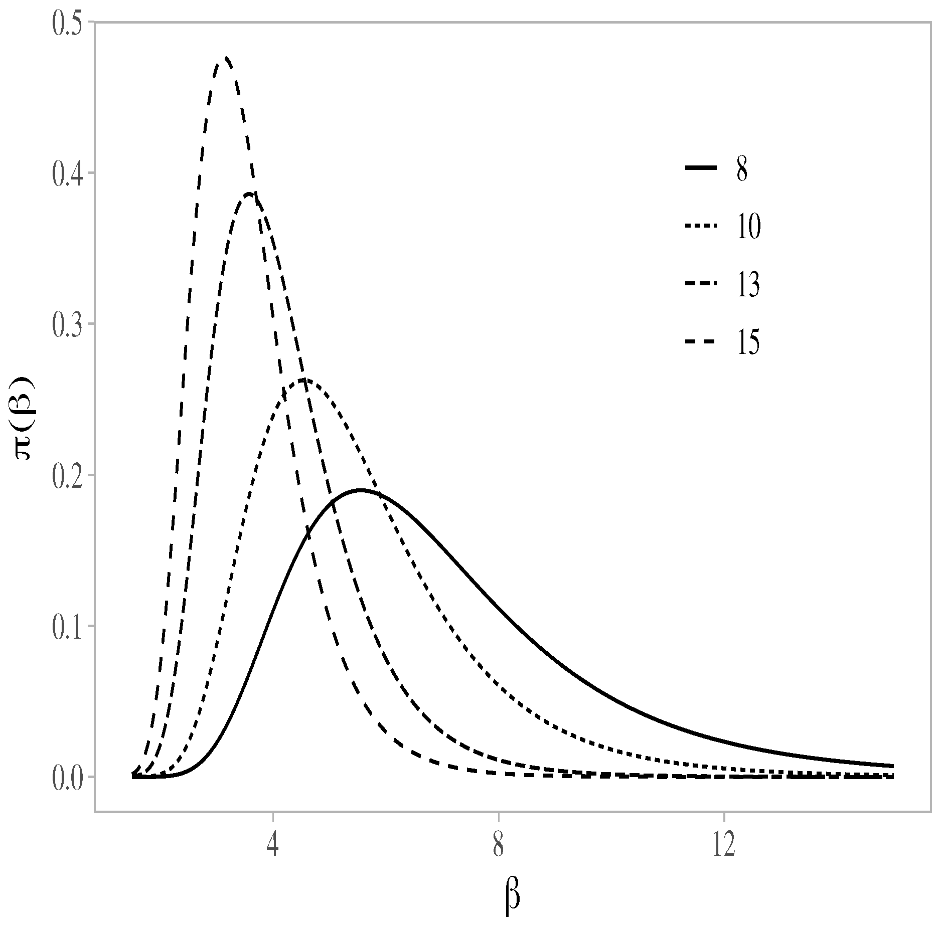
If $X\sim \mathrm{BS}(\alpha ,\beta )$, then $cX\sim \mathrm{BS}(\alpha ,c\beta )$, that is, the BS distribution is a homogeneous family;

P2:

If $X\sim \mathrm{BS}(\alpha ,\beta )$, then $1/X\sim \mathrm{BS}(\alpha ,1/\beta )$, that is, the BS distribution is invariant under the reciprocal transformation. This property can be important in financial applications.

2.2. Inference

Given a sample $\mathit{X}=(X_1,\dots ,X_n)$ and their observed values $\mathit{x}=(x_1,\dots ,x_n)$, modified moment estimates [25] for $\alpha$ and $\beta$ are expressed, respectively, as:

$$\tilde{\alpha }=\sqrt{2\left(\sqrt{\frac{{\overline{x}}_a}{{\overline{x}}_h}}-1\right)},\tilde{\beta }=\sqrt{{\overline{x}}_a{\overline{x}}_h},$$

(3)

where ${\overline{x}}_a$ is the sample arithmetic mean and ${\overline{x}}_h$ is the sample harmonic mean, that is,

$${\overline{x}}_a=\frac{1}{n}\sum _{i=1}^n{x}_i,{\overline{x}}_h={\left(\frac{1}{n}\sum _{i=1}^n\frac{1}{x_i}\right)}^{-1}.$$

In addition, the estimates $\tilde{\alpha }$ and $\tilde{\beta }$ are well defined because ${\overline{x}}_a\ge {\overline{x}}_h\ge 0$, that is, these estimates are always positive and mathematically well determined or unique. We may use $\tilde{\alpha }$ and $\tilde{\beta }$ as initial values in a sampling algorithm. Furthermore, the likelihood function obtained from the $\mathrm{BS}(\alpha ,\beta )$ probability density function satisfies:

$$\begin{array}{cc}\hfill \mathcal{L}(\alpha ,\beta ;{\mathit{x}}_n)\propto & {\displaystyle \frac{1}{{\left(\alpha \beta \right)}^n}\prod _{i=1}^n\left({\left(\frac{\beta }{x_i}\right)}^{1/2}+{\left(\frac{\beta }{x_i}\right)}^{3/2}\right)exp\left(-\frac{1}{2{\alpha }^2}\sum _{i=1}^n\left(\frac{x_i}{\beta }+\frac{\beta }{x_i}-2\right)\right).}\end{array}$$

For the parameters $\alpha$ and $\beta$ of the model, we consider proper prior distributions because the use of non-informative prior distributions yields an improper posterior distribution and continuous conjugate priors do not exist [26]. A possible choice of a prior distribution for $\beta$ is the inverse gamma (IG) distribution whose probability density function satisfies:

$$\pi \left(\beta \right)\propto {\beta }^{-(a_1+1)}exp\left(-\frac{b_1}{\beta }\right),\beta \in {\mathcal{R}}_{>0},$$

where $a_1$ and $b_1$ are positive and known constants (hyperparameters) of the IG distribution. We denote this as $\beta \sim \mathrm{IG}(a_1,b_1)$, that is, the IG distribution of parameters $a_1$ and $b_1$. We also assume an IG prior distribution for ${\alpha }^2$ with hyperparameters $a_2$ and $b_2$. Thus, the model can be written hierarchically as:

$$\begin{array}{c}{X}_i|\alpha ,\beta \stackrel{\mathrm{IID}}{\sim }\mathrm{BS}(\alpha ,\beta ),i=1,\dots ,n;\hfill \\ \beta \sim \mathrm{IG}(a_1,b_1),{\alpha }^2\sim \mathrm{IG}(a_2,b_2),\hfill \end{array}$$

where “IID” stands for independent and identically distributed. In this context, the conditional posterior distribution of ${\alpha }^2$ given $\beta$ and ${\mathit{x}}_n$ is stated as:

$${\alpha }^2|\beta ,{\mathit{x}}_n\sim \mathrm{IG}\left(\frac{n+1}{2}+a_2,\frac{1}{2}\sum _{i=1}^n\left(\frac{x_i}{\beta }+\frac{\beta }{x_i}-2\right)+b_2\right),$$

(4)

whereas the marginal posterior distribution of $\beta$ given ${\mathit{x}}_n$ can be obtained from:

$$\pi \left(\beta \right|{\mathit{x}}_n)\propto {\beta }^{-(n+a_1+1)}exp\left(\frac{b_1}{\beta }\right)\prod _{i=1}^n\left({\left(\frac{\beta }{x_i}\right)}^{1/2}+{\left(\frac{\beta }{x_i}\right)}^{3/2}\right){\left(\frac{1}{2}\sum _{i=1}^n\left(\frac{x_i}{\beta }+\frac{\beta }{x_i}-2\right)+b_2\right)}^{-\frac{(n+1)}{2}-a_2},$$

(5)

which is not a known distribution [26]. In this way, we use the random walk Metropolis–Hastings algorithm [27] to generate samples from the marginal posterior distribution of $\beta$ given ${\mathit{x}}_n$. Using this sampling algorithm and the posterior distribution defined in (4), we may generate values from the joint posterior distribution of ${\alpha }^2$ and $\beta$. For a given ${\mathit{x}}_n$, first, we generate values of $\beta$ from (5), and with them, we draw values of ${\alpha }^2$ using (4). Note that the parameter of interest $\mu$ is the mean of the BS distribution, which is a function of ${\alpha }^2$ and $\beta$. In order to obtain a random sample of the posterior distribution of $\mu$ given ${\mathit{x}}_n$, we may draw values from the joint posterior of ${\alpha }^2$ and $\beta$. Then, we apply the expression defined in (1) for each sampled pair of values.

3. Optimal Sample Size

In this section, we introduce the methodology to obtain the optimal sample size for estimating $\mu$ of the BS distribution under a decision-theoretic approach. Furthermore, we define the different loss functions to be considered.

3.1. Determining the Optimal Sample Size

We may approach the problem of determining the optimal sample size as a decision problem [4,28]. Given that $\mu$ is the parameter of interest, we specify a loss function $L(\mu ,d_n)$ based on a sample ${\mathit{X}}_n=(X_1,\dots ,X_n)$ and a decision function $d_n\equiv d_n\left({\mathit{X}}_n\right)$. For a given n and depending on the adopted loss function, the action $d_n\left({\mathit{x}}_n\right)$ consists of specifying a quantity (point inference case) representing an estimate for $\mu$ or two quantities (interval inference case) representing the lower and upper limits of a credible interval for $\mu$.

Let $\pi$ be associated with a prior distribution for the unknown parameter $\mu$ and $d_n$ be a decision function. Then, the Bayes risk [4] is defined as:

$$r(\pi ,d_n)={\int }_M{\int }_{{\mathcal{X}}^n}L(\mu ,d_n)g\left({\mathit{x}}_n\right|\mu )\pi \left(\mu \right)\mathrm{d}{\mathit{x}}_n\mathrm{d}\mu ,$$

(6)

where g is related to the sampling distribution for ${\mathit{X}}_n$ given $\mu$, M is the parameter space, and ${\mathcal{X}}_n$ is the sample space. The decision $d_n^{*}$ that minimizes $r(\pi ,d_n)$ among all the possible decisions $d_n$ is called the Bayes rule. In this context, we define the optimal sample size as the one that minimizes the total cost (TC) stated as:

$$\mathrm{TC}\left(n\right)=r(\pi ,d_n^{*})+C\left(n\right),$$

where $C\left(n\right)$ is a function representing the cost of sampling n observations. Here, we take $C\left(n\right)=cn$, where c is the per-unit cost for observing a unit in the population. Since it is not possible to compute $r(\pi ,d_n^{*})$ analytically, we use Monte Carlo simulations as an alternative to estimate $\mathrm{TC}\left(n\right)$ for each n.

Suppose that the order of the integration may be reversed in (6). Note that this reversal is possible whenever the conditions for the Fubini theorem are satisfied. In this case, as is known, minimizing the Bayes risk is equivalent to minimizing the posterior expected loss. Then, we have:

$$r(\pi ,d_n^{*})={\int }_{{\mathcal{X}}^n}\mathrm{E}\left[L(\mu ,d_n^{*})\right|{\mathit{x}}_n]g\left({\mathit{x}}_n\right)\mathrm{d}{\mathit{x}}_n,$$

so that we may estimate the minimized Bayes risk through the posterior expected value of the loss function applied to the Bayes rule $d_n^{*}$. This may be done as summarized in Algorithm 1.

After obtaining an estimate of $r(\pi ,d_n^{*})$, we added the respective sampling cost $cn$, which provided us an estimate of $\mathrm{TC}\left(n\right)$ for a given n. We apply this procedure for a grid of plausible values of n. For example, if we set this grid of values as $n=2,12,\dots ,82,92$, then we estimate $\mathrm{TC}\left(2\right),\mathrm{TC}\left(12\right),\dots ,\mathrm{TC}\left(82\right),\mathrm{TC}\left(92\right)$, respectively. The choice of the grid values is arbitrary, but as the distance between its consecutive elements is shorter, a better visualization is reached of the behavior of the TC. However, as this distance decreases, the required computer processing power also increases, as well as the time to compute all these estimates. Thus, the choice of this grid must consider all these settings.

Algorithm 1: Estimation of the minimized Bayes risk.

1  Set values for the hyperparameters, which reflect the prior knowledge about ${\alpha }^2$ and $\beta$. 2  Draw one value of ${\alpha }^2$ and one value of $\beta$ from the respective prior distributions, and compute the square root of ${\alpha }^2$. 3  Given $\alpha$ and $\beta$, generate a value of $X_i$ from the $\mathrm{BS}(\alpha ,\beta )$ distribution using (2), for $i=1,\dots ,n$, obtaining a sample ${\mathit{x}}_n=(x_1,\dots ,x_n)$. 4  Given ${\mathit{x}}_n$, collect a sample of size N (as large as possible) from the joint posterior distribution of ${\alpha }^2$ and $\beta$ as explained in Section 2, generating values $({\alpha }_j^2,{\beta }_j)$, for $j=1,\dots ,N$. 5  For $j=1,\dots ,N$, compute the posterior values ${\mu }_j$ using the generated values in Step 4 and the expression stated in (1). 6  Obtain the corresponding Bayes rule $d_n^{*}$ using the sample of the posterior distribution of $\mu$ generated in Step 5. 7  Use the values computed in Step 5 to estimate $\mathrm{E}\left[L(\mu ,d_n^{*})\right|{\mathit{x}}_n]$. 8  Repeat Steps 1–7 K times (as large as possible), generating K estimates of $\mathrm{E}\left[L(\mu ,d_n^{*})\right|{\mathit{x}}_n]$. 9  Take the average of the K estimates generated in Step 8 as an estimate of $r(\pi ,d_n^{*})$.

In Step 4 of Algorithm 1, when sampling from the marginal posterior distribution stated in (5), we consider a burn-in of 500 iterations and a thinning of 20 with a final number of iterations of 500. We use these 500 iterations to estimate the Bayes risk. A trace and autocorrelation plot for a lower value of the grid used for n is inspected. We expect the same or better behavior as n increased in the grid. All the trace plots showed a random behavior around a value, and in all the autocorrelation plots, the autocorrelations for almost all lags were zero. In each value of n in the grid, we estimate the Bayes risk ten times. We inspect the trace plots, autocorrelations plots, and the acceptance rate to set the burn-in, thinning, and final number of iterations as 500. All these inspection tools showed that such settings provide good results. If we increase these values, we may have the same or better behavior. However, we must consider the computational cost, which increases notoriously as these values increase. Then, taking all this into account, we decide to set 500 iterations. Due to the computational burden, other values were not tested, but we use triplicate values to show the stability of our results.

Consider the fitting proposed by [8] of the total cost curve established as:

$$\mathrm{tc}\left(n\right)=\frac{E}{{(1+n)}^G}+cn,$$

to the grid of values of n and the respective estimates of $\mathrm{TC}\left(n\right)$, denoted by $\mathrm{tc}\left(n\right)$, where E and G are parameters to be estimated. This curve may be linearized by means of:

$$log\left(\mathrm{tc}\right(n)-cn)=log\left(E\right)-Glog(1+n),$$

whereas the estimates of E and G can be computed by the least-squares method. In this setting, the optimal sample size ($n_{\mathrm{o}}$) is the integer closest to:

$${\left(\frac{\widehat{E}\widehat{G}}{c}\right)}^{1/(\widehat{G}+1)}-1,$$

where $\widehat{E}$ and $\widehat{G}$ are, respectively, the least-squares estimates of E and G.

3.2. Loss Functions

We consider five loss functions to determine the optimal sample size. The loss functions 1 and 2 may be used for point inference and are symmetric. The loss function 3 also may be used for point inference, but this loss function is asymmetric. The loss functions 4 and 5 may be used for interval inference. Such loss functions are defined below.

• L1: Loss Function 1. The first loss function is defined as:

  $$L(\mu ,d_n)=|\mu -d_n|,$$

  which is known as the absolute loss function. For this loss function, the Bayes rule $d_n^{*}$ is the median of the posterior distribution of $\mu$. Given a sample ${\mu }_j$, for $j=1,\dots ,N$, of the posterior distribution of $\mu$, an estimate of $\mathrm{E}\left[L(\mu ,d_n^{*})\right|{\mathit{x}}_n]$ may be obtained from ${\sum }_{j=1}^N|{\mu }_j-\widehat{d_n^{*}}|/N$, where $\widehat{d_n^{*}}$ is the median of the sample ${\mu }_j$, for $j=1,\dots ,N$.
• L2: Loss Function 2. Second, we consider the well-known quadratic loss function stated as:

  $$L(\mu ,d_n)={(\mu -d_n)}^2.$$

For this loss function, the Bayes rule $d_n^{*}$ corresponds to the posterior expected value of $\mu$, and in this case, $\mathrm{E}\left[L(\mu ,d_n^{*})\right|{\mathit{x}}_n]=\mathrm{Var}\left(\mu \right|{\mathit{x}}_n)$. Given a sample ${\mu }_j$, for $j=1,\dots ,N$, of the posterior distribution of $\mu$, an estimate of $\mathrm{E}\left[L(\mu ,d_n^{*})\right|{\mathit{x}}_n]$ may be obtained from the respective sample variance.

• L3: Loss Function 3. The loss functions L1 and L2 suffer from two disadvantages in practical applications: both are symmetric and unbounded. In the list of bounded loss functions that might be considered, we may include those suggested in [29,30]. However, in our case, these loss functions are not simple to deal with. Nevertheless, there is a simple well-know asymmetric loss function that we may consider. This is the linear exponential (known as LINEX) loss function given by:

  $$L(\mu ,d_n)=exp(\ell (d_n-\mu ))-\ell (d_n-\mu )-1,$$

  where $\ell \ne 0$. As ℓ increases positively, the overestimation is more costly than the underestimation. As ℓ increases negatively, the situation is reversed [31]. From p. 447 in [31], the Bayes rule for this loss function is established as:

  $$d_n^{*}=-\frac{1}{\ell }log\left(\mathrm{E}\left[\exp (-\ell \mu )|{\mathit{x}}_n\right]\right).$$

Given a sample ${\mu }_j$, for $j=1,\dots ,N$, of the posterior distribution of $\mu$, we may compute an estimate of $d_n^{*}$ through:

$$\widehat{d_n^{*}}=-\frac{1}{\ell }log\left(\frac{1}{N}\sum _{j=1}^N\exp (-\ell {\mu }_j)\right).$$

For the LINEX function, we have that [5]:

$$\mathrm{E}\left[L(\mu ,d_n^{*})\right|{\mathit{x}}_n]=\ell \left(\mathrm{E}\left[\mu \right|{\mathit{x}}_n]-d_n^{*}\right).$$

An estimate of $\mathrm{E}\left[L(\mu ,d_n^{*})\right|{\mathit{x}}_n]$ may be obtained from:

$$\widehat{\mathrm{E}}\left[L(\mu ,d_n^{*})\right|{\mathit{x}}_n]=\ell \left(\frac{1}{N}\sum _{j=1}^N{\mu }_j-\widehat{d_n^{*}}\right).$$

• L4: Loss Function 4. The fourth function is defined as:

  $$L(\mu ,d_n)=\rho \tau +{(a-\mu )}^{+}+{(\mu -b)}^{+},$$

  (7)

  where $0<\rho <1$ is a weight, $\tau =(b-a)/2$ is the half-length of the desired interval, and the function $x^{+}$ is equal to x if $x>0$ and equal to zero, otherwise. Note that as $\tau$ decreases, the interval is narrower. The terms ${(a-\mu )}^{+}$ and ${(\mu -b)}^{+}$ are included to penalized intervals that do not contain the parameter of interest $\mu$. These terms are equal to zero if $\mu \in [a,b]$ and increase as $\mu$ moves away from the interval. Note that the loss function given in (7) is a weighted sum of two terms, $\tau$ and ${(a-\mu )}^{+}+{(\mu -b)}^{+}$, where the weights are $\rho$ and one, respectively. The Bayes rule $d_n^{*}$ corresponds to taking a and b as the 100$(\rho /2)$th and 100$(1-\rho /2)$th quantiles of the posterior distribution of $\mu$ [8,32]. If we consider this loss function applied to the Bayes rule, we have that:

  $$\mathrm{E}\left[L(\mu ,d_n^{*})\right|{\mathit{x}}_n]=\mathrm{E}\left[\mu {\delta }_{\mu }\left(A_{b^{*}}\right)\right|{\mathit{x}}_n]-\mathrm{E}\left[\mu {\delta }_{\mu }\left(A_{a^{*}}\right)\right|{\mathit{x}}_n],$$

  where $A_{b^{*}}=[b^{*},\infty )$, $A_{a^{*}}=(0,a^{*}]$, $a^{*}$ and $b^{*}$ are the corresponding bounds of the Bayes rule $d_n^{*}$, whereas ${\delta }_{\mu }$ is the indicator function. Given a sample ${\mu }_j$, for $j=1,\dots ,N$, of the posterior distribution of $\mu$, an estimate of $\mathrm{E}\left[L(\mu ,d_n^{*})\right|{\mathit{x}}_n]$ may be obtained from:

  $$\widehat{\mathrm{E}}\left[L(\mu ,d_n^{*})\right|{\mathit{x}}_n]=\frac{1}{N}\sum _{j=1}^N({\mu }_j{\delta }_{{\mu }_j}\left(A_{b^{*}}\right)-{\mu }_j{\delta }_{{\mu }_j}\left(A_{a^{*}}\right)).$$
• L5: Loss Function 5. The fifth and last loss function considered here is expressed as:

  $$L(\mu ,d_n)=\gamma \tau +\frac{{(\mu -m)}^2}{\tau },$$

  (8)

  where $\gamma >0$ is a fixed constant and $m=(a+b)/2$ is the center of the credible interval. The first term defined in (8) involves the half-width of the interval, and the second term is the square of the distance between the parameter of interest $\mu$ and the center of the interval, which is divided by the half-width to maintain the same measurement unit of the first term. The weights attributed to each term stated in (8) are $\gamma$ and one, respectively. If $\gamma <1$, we attribute the largest weight to the second term; if $\gamma >1$, the situation is reversed; and if $\gamma =1$, the two terms have the same weight. For this loss function, the Bayes rule $d_n^{*}$ corresponds to the quantities that define the interval $[a^{*},b^{*}]=[m^{*}-{SD}_{\gamma },m^{*}+{SD}_{\gamma }]$, where $m^{*}=\mathrm{E}\left[\mu \right|{\mathit{x}}_n]$ and ${SD}_{\gamma }={\gamma }^{-1/2}{\left(\mathrm{Var}\left(\mu \right|{\mathit{x}}_n)\right)}^{1/2}$, that is, the corresponding standard deviation [4,8,32]. In this case, we have that:

  $$\mathrm{E}\left[L(\mu ,d_n^{*})\right|{\mathit{x}}_n]=2{\gamma }^{1/2}\sqrt{\mathrm{Var}\left(\mu \right|{\mathit{x}}_n)}.$$

  (9)

Given a sample ${\mu }_j$, for $j=1,\dots ,N$, of the posterior distribution of $\mu$, an estimate of $\mathrm{E}\left[L(\mu ,d_n^{*})\right|{\mathit{x}}_n]$ may be obtained from the sample variance and the expression (9).

4. Computational Aspects and Empirical Applications

In this section, we provide the characteristics of the computer that was used in our study. Also, we show the capabilities and features of a new R package which is named samplesizeBS [22] and is available from GitHub at https://github.com/santosneto/samplesizeBS (accessed on 21 May 2021). The capabilities of the samplesizeBS package allow us to calculate an optimal sample size when estimating the BS mean and generate random numbers of the joint posterior BS/IG distribution. This section finishes with an empirical application based on real data.

4.1. Computer Characteristics

The characteristics of the Cluster Euler, used when calculating the optimal sample size in Section 4.3, are available at http://www.cemeai.icmc.usp.br/Euler/index.html (accessed on 22 May 2021). The other numerical results presented in the simple example of Section 4.2, and the illustrative example with real data of Section 4.4, were obtained by a computer with the following characteristics: (i) OS: Linux Mint 19.3 Cinnamon; (ii) RAM: 7.7 GiB; and (iii) processor: Intel Core i5-7200U [email protected] x 2. In addition, the following tools and programming languages were used: (i) development tool –IDE–: RStudio Version (1.3.1093); and (ii) statistical software: R. Note that, in the simple example regarding the use of the function bss.dt.bs(), the elapsed time was: 19 m 48 s.

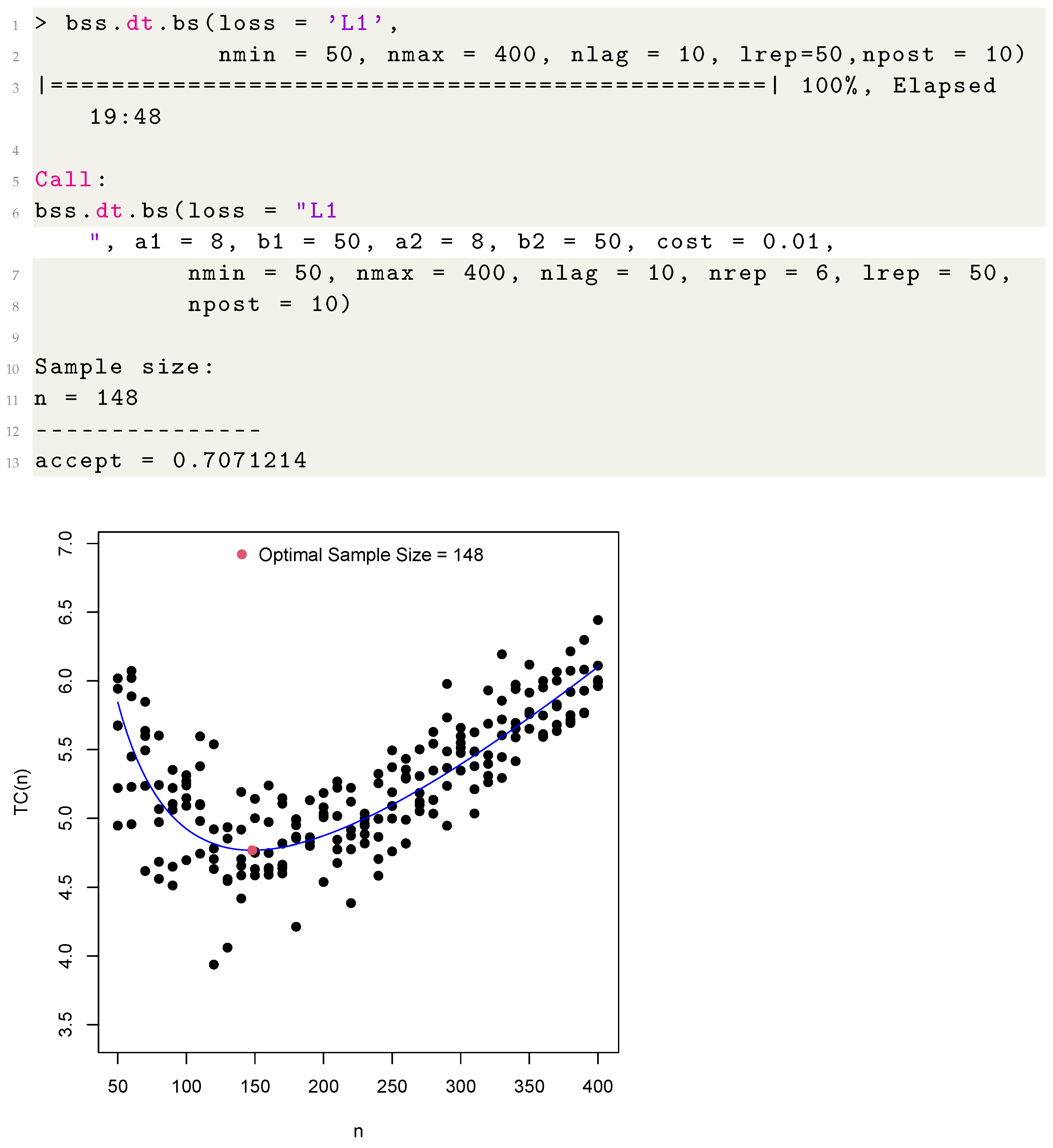
4.2. The samplesizeBS Functions

In

Table 1. Functions and the respective outputs of the samplesizeBS package.

Function	Output
rbs()	A sample of size n from the BS distribution
logp.beta()	The logarithm of the marginal posterior distribution of $\beta$
rbeta.post()	A random sample from the marginal posterior distribution of $\beta$ using the random walk Metropolis–Hastings algorithm
bss.dt.bs()	An integer representing the optimal sample size for estimating $\mu$ of the BS distribution and the acceptance rate for the random walk Metropolis–Hastings algorithm

, we present the details of the functions contained in the samplesizeBS package.

In order to determinate the BS optimal sample size, we use the function bss.dt.bs(). In the example below, we calculate the optimal sample size considering the loss function L1, with $a_1=a_2=8$, $b_1=b_2=50$, and $c=0.01$. The function also returns the graph with the sample size (n) versus the $\mathrm{TC}\left(n\right)$ of sampling, that is, $\mathrm{TC}\left(n\right)$ takes into account both the cost of sampling n observations and the cost of inference through the loss function. In this way, the optimal sample size is the value that minimizes the total cost (see Figure 1).

4.3. Optimal Sample Sizes

Next, we calculate the optimal sample size assuming different scenarios. For the hyperparameters of the prior distribution of $\beta$, we take $b_1=50$ and $a_1=8,10,13,15$. With these values, we have different degrees of prior information (see Figure 2). For the prior distribution of ${\alpha }^2$, we set $a_2=a_1$ and $b_2=b_1$. We consider $c=0.001,0.01,0.1$ for the per-unit cost. For the loss function L3, we take $\ell =0.50,1.00,2.00$, for L4, $\rho =0.01,0.05,0.10$, and for L5, $\gamma =0.25,0.50,1.00$. For each combination of these values, we compute the optimal sample size $n_{\mathrm{o}}$ for estimating $\mu$. The average acceptance rate for the Metropolis–Hastings algorithm in all these combinations was $\approx 70\%$. Since the proposed methodology is based on simulation methods, we obtain $n_{\mathrm{o}}$ in triplicate and observe the difference for the three values.

Table 2. Optimal sample sizes $n_{\mathrm{o}}$ (in triplicate) when estimating the mean of the BS distribution via five different loss functions.

$\mathit{\rho }/\mathit{\gamma }/\mathit{\ell }$	${\mathit{a}}_1=8$			${\mathit{a}}_1=10$			${\mathit{a}}_1=13$			${\mathit{a}}_1=15$
	$\mathit{c}=\mathbf{0.001}$	$\mathit{c}=\mathbf{0.01}$	$\mathit{c}=\mathbf{0.1}$	$\mathit{c}=\mathbf{0.001}$	$\mathit{c}=\mathbf{0.01}$	$\mathit{c}=\mathbf{0.1}$	$\mathit{c}=\mathbf{0.001}$	$\mathit{c}=\mathbf{0.01}$	$\mathit{c}=\mathbf{0.1}$	$\mathit{c}=\mathbf{0.001}$	$\mathit{c}=\mathbf{0.01}$	$\mathit{c}=\mathbf{0.1}$
	Loss function L1
	651	117	23	436	80	13	267	47	9	210	36	6
	641	121	22	429	77	14	267	47	8	209	36	6
	627	140	21	429	77	13	268	47	8	209	37	6
	Loss function L2
	2096	641	176	1130	317	108	542	144	33	381	88	21
	2129	697	200	1198	326	97	558	138	42	380	89	23
	2075	622	218	1182	292	81	530	139	32	360	89	21
	Loss function L3
$\ell =2.00$	1787	354	61	1111	229	41	631	138	24	467	101	18
	1826	363	62	1115	235	40	640	135	25	468	101	18
	1820	352	61	1112	229	41	616	134	25	454	97	19
$\ell =1.00$	929	190	34	553	122	22	310	69	13	226	51	9
	924	197	34	556	122	22	311	69	13	227	51	9
	925	190	34	552	116	22	308	67	13	222	49	9
$\ell =0.50$	465	101	19	281	63	12	153	35	7	111	25	5
	463	101	19	275	63	12	155	35	7	111	25	4
	471	99	18	275	59	12	146	33	6	105	23	4
	Loss function L4
$\rho =0.10$	279	53	9	175	31	7	103	18	3	79	14	2
	271	54	10	171	31	6	106	18	3	79	14	2
	284	53	10	168	33	5	103	18	3	80	14	2
$\rho =0.05$	187	37	8	118	22	4	70	13	2	54	9	0
	197	37	8	121	22	4	71	12	2	55	9	0
	184	40	7	121	22	4	71	13	2	55	9	0
$\rho =0.01$	82	18	3	54	9	0	30	5	0	22	4	0
	85	19	3	52	9	0	29	5	0	22	4	0
	83	18	3	49	9	0	30	5	0	22	4	0
	Loss function L5
$\gamma =1.00$	1461	271	51	899	171	30	556	103	18	441	78	13
	1472	292	55	942	162	31	561	99	18	438	78	13
	1460	282	56	883	162	30	554	101	18	433	78	13
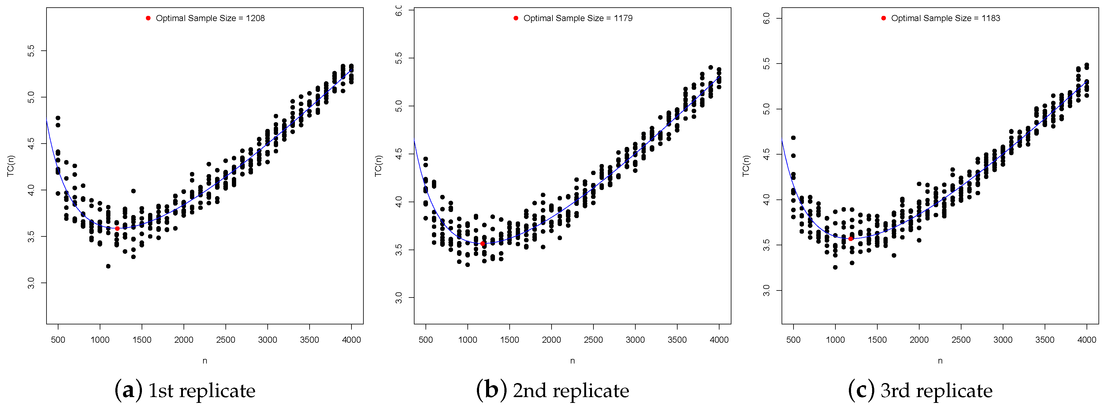
$\gamma =0.50$	1208	203	39	684	132	23	427	78	14	337	59	10
	1179	201	38	690	130	23	434	78	14	335	59	10
	1183	213	42	693	134	24	436	80	14	338	60	10
$\gamma =0.25$	796	166	32	538	106	18	333	59	10	259	46	8
	859	171	30	540	99	19	331	62	11	260	47	8
	894	167	32	531	101	18	333	60	10	260	46	8

reports the optimal sample sizes computed with these settings. In addition, $n_{\mathrm{o}}$ may be reached via the following link, which also presents a graph with the fitted curve:

https://santosneto.shinyapps.io/samplesizeBSapp (accessed on 21 May 2021).

Note that values of the hyperparameters are fixed according to the practitioner’s knowledge for the parameters ${\alpha }^2$ and $\beta$ (see Step 1 of Algorithm 1). For example, if we set the hyperparameters as $a_1=8$ and $b_1=50$, it means that our prior knowledge indicates the most likely values for $\beta$ in the interval between the numbers 3 and 5 (see Figure 2) and similarly for the parameter ${\alpha }^2$. Thus, for instance, if the practitioner’s prior knowledge is that the possible values for $\beta$ (and/or ${\alpha }^2$) are in the interval between the numbers 6 and 9, the practitioner must set the values of the hyperparameters (parameters of the IG distribution) such that the greatest mass of probability of the IG distribution is in the interval between the numbers 6 and 9.

4.4. Illustrative Example

A practical application of the methodology to compute the optimal sample size when estimating the mean of the BS distribution is illustrated here with one example. In this example, we consider a data set composed by 46 observations given in [33] and available in the samplesizeBS package [22]. These observations correspond to maintenance data on active repair times (in hours) for an airborne communications transceiver. Let $x_i$ be the observation i of this data set associated with the random variable $X_i\sim \mathrm{BS}(\alpha ,\beta )$.

First, we estimate $\alpha$ and $\beta$ using the modified moment method defined in (3), which result in $\tilde{\alpha }=1.25$ and $\tilde{\beta }=2.02$, respectively. In this way, we can set IG prior distributions for ${\alpha }^2$ and $\beta$ with $a_1=a_2=15$ and $b_1=b_2=50$ (see Figure 2). Hence, if our interest is in obtaining a credible interval for $\mu$ considering the loss function L5, with $\gamma =0.25$ and $c=0.01$, the optimal sample size may be obtained from Table 2, which is $n_{\mathrm{o}}=46$.

Now, we generate 1000 observations from the posterior distribution of $\mu$ and estimate the mean and variance of the respective posterior distribution through the sample mean and variance, respectively. With these estimates, we obtain a credible interval for $\mu$ given by [2.108; 3.939].

5. Discussion, Conclusions and Future Research

We proposed a methodology to compute the optimal sample size for estimating the mean of the Birnbaum–Saunders distribution, a widely applied and studied distribution in several areas of science. We considered five different loss functions, which allowed us to perform both point and interval inference for the parameter of interest.

An advantage of the proposed methodology is that the per-unit cost, represented by c, is explicitly taken into account. When the cost c is fixed and $b_1=50$, the optimal sample size $n_{\mathrm{o}}$ decreases as $a_1$ increases (or as the prior variance decreases), as expected, since in such a case, the prior knowledge increases as $a_1$ increases. This occurred with all loss functions considered in our study. For $b_1=50$ and $a_1$ fixed, $n_{\mathrm{o}}$ also decreases as c increases, but the sampling total cost increases. For example, if we take the loss function L1, $a_1=8$ and $c=0.001$, the corresponding $n_{\mathrm{o}}$ is 651 (see Table 2), which generates a sampling cost of $C\left(651\right)=0.001\times 651=0.651$, whereas if we take $c=0.1$, the corresponding $n_{\mathrm{o}}$ is 23 (see Table 2), which produces a sampling cost of $C\left(23\right)=0.1\times 23=2.3$. For the loss function L3, $n_{\mathrm{o}}$ increases as ℓ increases, if we consider $a_1$ and c fixed, which makes sense since overestimation is more costly as ℓ increases. For the loss function L4, when $\rho$ increases, $n_{\mathrm{o}}$ also increases, if we consider $a_1$ and c fixed. This makes sense because $\rho$ is the weight attributed to the term $\tau$ in L4, a term related to the length of the credible interval. In addition, when $\rho$ increases, we expect longer credible intervals, and consequently, the probability of the respective interval decreases. The same is valid for $\gamma$ in the loss function L5, but in this case, the decreasing of the corresponding credible interval is easily noted by the presence of the term ${\gamma }^{-1/2}$ in the expression of the respective Bayes rule. When $\gamma$ increases, this term shrinks the length of the interval.

Since the proposed methodology was based on simulations, we obtained the value of $n_{\mathrm{o}}$ in triplicate for each scenario of values of $a_1$, c, ℓ, $\rho$, and $\gamma$. We observed that the largest discrepancies in the scenarios occurred for $a_1=8$. However, these discrepancies decreased as $a_1$ increased, or when the prior variance decreased. This also occurred when $c=0.001$ and/or when we considered the loss function L2. In general, the discrepancy was close to zero, but if a large discrepancy occurs, we suggest visually inspecting the graph of the fitted curves and taking the value of $n_{\mathrm{o}}$ that corresponds to the best fit. Nevertheless, if all the curves fit visually well, we suggest using the median of the values obtained for $n_{\mathrm{o}}$. In our case, we obtained the values of $n_{\mathrm{o}}$ in triplicate, as mentioned. For example, in Figure 3, under the loss function L5 with $a_1=8$, $c=0.001$, and $\gamma =0.50$, the values of $n_{\mathrm{o}}$ were 1208, 1179, and 1183. Since there was a discrepancy between these values and the fittings of the curves were visually suitable, in this case, we suggest using $n_{\mathrm{o}}=1183$. Note that we have optimal sample sizes equal to zero in Table 2 in some scenarios, which means that it is not worth sampling in these cases because the sampling cost outweighs the decreasing of the minimized Bayes risk. This was also observed in [2,6].

We recall that the objective of the present investigation was to calculate the optimal sample size when estimating the mean of the Birnbaum–Saunders distribution. Simulation experiments should be performed to study the relative bias of the estimator of the mean (or the width of the corresponding interval estimate). A sensitivity analysis considering such simulation experiments would also be helpful. However, as mentioned, our methodology uses very intensive computational resources, which limits the implementation of such experiments. In addition, we plan to consider different priors for the parameters and to examine the robustness and the sensitivity of the results. Moreover, we are interested in studying the possibility of using bounded loss functions and other sampling algorithms.

The relevance of calculating sample sizes in statistics is undeniable. Another important challenge to be implemented is related to calculating the sample size when estimating the Birnbaum–Saunders mean (or other parameters) under more complex modeling structures, such as regression, temporal, spatial, functional, PLS, and errors-in-variables settings [34,35,36,37,38]. We hope to report findings associated with these open aspects in future research.

References

- Spiegelhalter, D.J.; Abrams, K.R.; Myles, J.P. Bayesian Approaches to Clinical Trials and Health-Care Evaluation; Wiley: Chichester, UK, 2004. [Google Scholar]
- Etzioni, R.; Kadane, J.B. Optimal experimental design for another’s analysis. J. Am. Stat. Assoc. 1993, 88, 1404–1411. [Google Scholar] [CrossRef]
- Sahu, S.K.; Smith, T.M.F. A Bayesian method of sample size determination with practical applications. J. R. Stat. Soc. A 2006, 169, 235–253. [Google Scholar] [CrossRef]
- Parmigiani, G.; Inoue, L. Decision Theory: Principles and Approaches; Wiley: New York, NY, USA, 2009. [Google Scholar]
- Islam, A.F.M.S.; Pettit, L.I. Bayesian sample size determination using LINEX loss and linear cost. Commun. Stat. Theory Methods 2012, 41, 223–240. [Google Scholar] [CrossRef]
- Islam, A.F.M.S.; Pettit, L.I. Bayesian sample size determination for the bounded LINEX loss function. J. Stat. Comput. Simul. 2014, 84, 1644–1653. [Google Scholar] [CrossRef]
- Santis, F.D.; Gubbiotti, S. A decision-theoretic approach to sample size determination under several priors. Appl. Stoch. Model. Bus. Ind. 2017, 33, 282–295. [Google Scholar] [CrossRef]
- Costa, E.G. Sample Size for Estimating the Organism Concentration in Ballast Water: A Bayesian Approach. Ph.D. Thesis, Department of Statistics, Universidade de São Paulo, São Paulo, Brazil, 2017. (In Portuguese). [Google Scholar]
- Birnbaum, Z.W.; Saunders, S.C. A new family of life distributions. J. Appl. Probab. 1969, 6, 319–327. [Google Scholar] [CrossRef]
- Bourguignon, M.; Leao, J.; Leiva, V.; Santos-Neto, M. The transmuted Birnbaum–Saunders distribution. REVSTAT Stat. J. 2017, 15, 601–628. [Google Scholar]
- Mazucheli, M.; Leiva, V.; Alves, B.; Menezes, A.F.B. A new quantile regression for modeling bounded data under a unit Birnbaum–Saunders distribution with applications in medicine and politics. Symmetry 2021, 13, 682. [Google Scholar] [CrossRef]
- Santos-Neto, M.; Cysneiros, F.J.A.; Leiva, V.; Barros, M. Reparameterized Birnbaum–Saunders regression models with varying precision. Electron. J. Stat. 2016, 10, 2825–2855. [Google Scholar] [CrossRef]
- Reyes, J.; Barranco-Chamorro, I.; Gallardo, D.I.; Gomez, H.W. Generalized modified slash Birnbaum—Saunders distribution. Symmetry 2018, 10, 724. [Google Scholar] [CrossRef]
- Gomez-Deniz, E.; Gomez, L. The Rayleigh Birnbaum Saunders distribution: A general fading model. Symmetry 2020, 12, 389. [Google Scholar] [CrossRef]
- Desousa, M.; Saulo, H.; Leiva, V.; Santos-Neto, M. On a new mixture-based regression model: Simulation and application to data with high censoring. J. Stat. Comput. Simul. 2020, 90, 2861–2877. [Google Scholar] [CrossRef]
- Sanchez, L.; Leiva, V.; Galea, M.; Saulo, H. Birnbaum–Saunders quantile regression and its diagnostics with application to economic data. Appl. Stoch. Models Bus. Ind. 2021, 37, 53–73. [Google Scholar] [CrossRef]
- Villegas, C.; Paula, G.A.; Leiva, V. Birnbaum–Saunders mixed models for censored reliability data analysis. IEEE Trans. Reliab. 2011, 60, 748–758. [Google Scholar] [CrossRef]
- Marchant, C.; Leiva, V.; Cysneiros, F.J.A. A multivariate log-linear model for Birnbaum–Saunders distributions. IEEE Trans. Reliab. 2016, 65, 816–827. [Google Scholar] [CrossRef]
- Arrue, J.; Arellano, R.; Gomez, H.W.; Leiva, V. On a new type of Birnbaum–Saunders models and its inference and application to fatigue data. J. Appl. Stat. 2020, 47, 2690–2710. [Google Scholar] [CrossRef]
- Balakrishnan, N.; Kundu, D. Birnbaum–Saunders distribution: A review of models, analysis, and applications. Appl. Stoch. Model. Bus. Ind. 2019, 35, 4–49. [Google Scholar] [CrossRef]
- Bourguignon, M.; Ho, L.L.; Fernandes, F.H. Control charts for monitoring the median parameter of Birnbaum–Saunders distribution. Qual. Reliab. Eng. Int. 2020, 36, 1333–1363. [Google Scholar] [CrossRef]
- Costa, E.G.; Santos-Neto, M.; Leiva, V. samplesizeBS: Bayesian Sample Size in a Decision-Theoretic Approach for the Birnbaum–Saunders, R Package Version 1.1-1; 2020. Available online: www.github.com/santosneto/samplesizeBS (accessed on 21 May 2021).
- Aykroyd, R.G.; Leiva, V.; Marchant, C. Multivariate Birnbaum–Saunders distributions: Modelling and applications. Risks 2018, 6, 21. [Google Scholar] [CrossRef]
- Leiva, V. The Birnbaum–Saunders Distribution; Academic Press: New York, NY, USA, 2016. [Google Scholar]
- Ng, H.; Kundu, D.; Balakrishnan, N. Modified moment estimation for the two-parameter Birnbaum–Saunders distribution. Comput. Stat. Data Anal. 2003, 43, 283–298. [Google Scholar] [CrossRef]
- Wang, M.; Sun, X.; Park, C. Bayesian analysis of Birnbaum–Saunders distribution via the generalized ratio-of-uniforms method. Comput. Stat. 2016, 31, 207–225. [Google Scholar] [CrossRef]
- Leiva, V.; Ruggeri, F.; Saulo, H.; Vivanco, J.F. A methodology based on the Birnbaum–Saunders distribution for reliability analysis applied to nano-materials. Reliab. Eng. Syst. Saf. 2017, 157, 192–201. [Google Scholar] [CrossRef]
- Raiffa, H.; Schlaifer, R. Applied Statistical Decision Theory; Harvard University Press: Boston, MA, USA, 1961. [Google Scholar]
- Spiring, F.A. The reflected normal loss function. Can. J. Stat. 1993, 21, 321–330. [Google Scholar] [CrossRef]
- Leung, B.P.K.; Spiring, F.A. The inverted beta loss function: Properties and applications. IEE Trans. 2002, 34, 1101–1109. [Google Scholar] [CrossRef]
- Zellner, A. Bayesian estimation and prediction using asymmetric loss functions. J. Am. Stat. Assoc. 1986, 81, 446–451. [Google Scholar] [CrossRef]
- Rice, K.M.; Lumley, T.; Szpiro, A.A. Trading Bias for Precision: Decision Theory for Intervals and Sets. Working Paper 336, UW Biostatistics. 2008. Available online: https://biostats.bepress.com/uwbiostat/paper336/ (accessed on 21 May 2021).
- Hsieh, H.K. Estimating the critical time of the inverse Gaussian hazard rate. IEEE Trans. Reliab. 1990, 39, 342–345. [Google Scholar] [CrossRef]
- Puentes, R.; Marchant, C.; Leiva, V.; Figueroa, J.I.; Ruggeri, F. Predicting PM2.5 and PM10 levels during critical episodes management in Santiago, Chile, with a bivariate Birnbaum–Saunders log-linear model. Mathematics 2021, 9, 645. [Google Scholar] [CrossRef]
- Leiva, V.; Saulo, H.; Souza, R.; Aykroyd, R.G.; Vila, R. A new BISARMA time series model for forecasting mortality using weather and particulate matter data. J. Forecast. 2021, 40, 346–364. [Google Scholar] [CrossRef]
- Martinez, S.; Giraldo, R.; Leiva, V. Birnbaum–Saunders functional regression models for spatial data. Stoch. Environ. Res. Risk Assess. 2019, 33, 1765–1780. [Google Scholar] [CrossRef]
- Huerta, M.; Leiva, V.; Liu, S.; Rodriguez, M.; Villegas, D. On a partial least squares regression model for asymmetric data with a chemical application in mining. Chemom. Intell. Lab. Syst. 2019, 190, 55–68. [Google Scholar] [CrossRef]
- Carrasco, J.M.F.; Finiga, J.I.; Leiva, V.; Riquelme, M.; Aykroyd, R.G. An errors-in-variables model based on the Birnbaum–Saunders and its diagnostics with an application to earthquake data. Stoch. Environ. Res. Risk Assess. 2020, 34, 369–380. [Google Scholar] [CrossRef]