Article

A Damage Model to Trabecular Bone and Similar Materials: Residual Resource, Effective Elasticity Modulus, and Effective Stress under Uniaxial Compression

by
Gennady Kolesnikov
1,* and
Rudolf Meltser
2
1
Institute of Forestry, Mining and Construction Sciences, Petrozavodsk State University, Lenin pr., 33, 185910 Petrozavodsk, Russia
2
Medical Institute, Petrozavodsk State University, Lenin pr., 33, 185910 Petrozavodsk, Russia
*
Author to whom correspondence should be addressed.
Symmetry 2021, 13(6), 1051; https://doi.org/10.3390/sym13061051
Submission received: 8 April 2021 / Revised: 4 June 2021 / Accepted: 8 June 2021 / Published: 10 June 2021
(This article belongs to the Special Issue Applied Mechanics, Engineering and Modeling)

Abstract

:
Experimental research of bone strength remains costly and limited for ethical and technical reasons. Therefore, to predict the mechanical state of bone tissue, as well as similar materials, it is desirable to use computer technology and mathematical modeling. Yet, bone tissue as a bio-mechanical object with a hierarchical structure is difficult to analyze for strength and rigidity; therefore, empirical models are often used, the disadvantage of which is their limited application scope. The use of new analytical solutions overcomes the limitations of empirical models and significantly improves the way engineering problems are solved. Aim of the paper: the development of analytical solutions for computer models of the mechanical state of bone and similar materials. Object of research: a model of trabecular bone tissue as a quasi-brittle material under uniaxial compression (or tension). The new ideas of the fracture mechanics, as well as the methods of mathematical modeling and the biomechanics of bone tissues were used in the work. Compression and tension are considered as asymmetric mechanical states of the material. Results: a new nonlinear function that simulates both tension and compression is justified, analytical solutions for determining the effective and apparent elastic modulus are developed, the residual resource function and the damage function are justified, and the dependences of the initial and effective stresses on strain are obtained. Using the energy criterion, it is proven that the effective stress continuously increases both before and after the extremum point on the load-displacement plot. It is noted that the destruction of bone material is more likely at the inflection point of the load-displacement curve. The model adequacy is explained by the use of the energy criterion of material degradation. The results are consistent with the experimental data available in the literature.

1. Introduction

This article discusses the issues of biomechanical modeling of trabecular bone tissue using new ideas of fracture mechanics. It is taken into account that the structure of bone tissue in the process of its formation and renewal naturally and optimally adapts to biomechanical functions [1,2]. Moreover, bone cells are periodically, but not synchronously, updated, which determines the dependence of the strength of structural units on the stage of renewal. In most cases, bone tissue is a very complex object, the study of which will not stop for a long time [3,4].
From the point of view of mechanics, at the macro level, bone tissue is an inhomogeneous anisotropic porous material. Structural units (including the walls between the pores) interact with each other, resisting mechanical influences, so a bone sample with a characteristic size of a few millimeters or more can be considered as a certain mechanical system consisting of hierarchically ordered nano-, micro-, and meso-scale structural units [5,6,7]. The characteristic sizes of bone structural units are in the range from 1 nanometer to 500 micrometers [8]. The hierarchical heterogeneous structure of bone tissue provides high resistance to destruction [9]. Despite this, a sufficiently large mechanical impact on the bone is accompanied by the appearance of micro-cracks [10], the initial length of which usually corresponds to the characteristic size of the structural element of the bone [8]. The development of micro-cracks leads to a weakening of the connections between the bone structural units, as well as to their partial or complete exclusion from the number of fully functioning bone components. Accordingly, the number of intact structural units decreases, and the average load on each of them increases. Consequently, stresses and deformations in the material of structural units increase, which can lead to bone fractures. The risk of fracture can be defined as the ratio of the actual stress to the ultimate stress; using this ratio allows you to abstract from the specific shape of the bone [11].
A number of experimental methods for determining the ultimate stress are known: tests of bone tissue samples for compression, tension, three- or four-point bending, shear, and torsion [6]. In our work, we focus on the external manifestations of the mechanical properties of bone tissue under tension and compression, namely, on the load–displacement and stress–strain ratios. In other words, from a methodological point of view, the phenomenological approach is used to construct a mathematical model of the behavior of bone tissue in the process of testing samples for compression and tension. From the physical point of view, the model is based on the use of key concepts of fracture mechanics. To verify the results of the mathematical modeling, experimental data known from the literature were used.

1.1. The Load–Displacement Interrelationships under Uniaxial Loading

Uniaxial compression and tension tests are a key source of primary information for theoretical generalizations. Compression tests are widely used to determine the strength and stiffness of bone tissue [12,13,14]. Tensile tests are somewhat more complicated [6,15,16]. The key test results are load–displacement ratios, which integrally reflect both the explicit and implicit influence of various factors, including sample size and shape, material porosity, moisture, anisotropy, age, bone pathology, and the rate of load change. It is important to note that the load–displacement relations characterize the behavior of the sample or the entire bone as a structure, but these relations to a lesser extent reflect the properties of the material of the structural units of the bone, as well as the evolution of micro-cracks [10]. Therefore, it is important to find the relationship between the “load–displacement” ratio and the “stress–strain” ratio, taking into account the material damage during loading.
A typical load–displacement plot for the trabecular bone [13] is schematically shown in Figure 1a. Note that the asymmetric plots of the function y = A sin ( k x ) (Figure 1b) at some values of A and k over a limited interval are almost similar in appearance to the experimental stress–strain plots [12,13]. It is important that such an analogy induces a hypothesis about the possibility of a mathematical description of the asymmetric load–displacement plot by only one simple function; the justification and implementation of this possibility is discussed below, in a separate section.
As noted above, the load–displacement ratios depend on the properties of the material at the tissue level (at the micro level), but these ratios are more characteristic of the properties of the bone sample as a structure (at the macro level). Tests of samples at the macro level are not so difficult in comparison with tests of the micro-samples (for example, individual trabeculae) [6,17]. The problem is to determine the mechanical properties of the material of the structural unit of bone, since the above-mentioned characteristic dimensions of these units are very small [8]. At the same time, reducing the size of the sample does not lead to the solution of the problem, which follows from the results of work [17] and shows that some trabeculae can be strongly stressed while others are practically unloaded even within the volume of 1 mm 3 . Variations in strength can be explained by the changeable architecture of the trabecular system [17], changes in the age of bone cells [18,19,20], and other features [1,2,8,11].
Therefore, taking into account the above, at the conceptual level, we postulate that the experimental load–displacement relationships integrally reflect the influence of all the factors accompanying the tests. Therefore, the experimental load–displacement relationships are a key source of primary information necessary for further and more detailed analyses of stress and strain.

1.2. The Stress–Strain Ratio

The apparent stress is determined using a continuum model that does not take into account the evolution of cracks and the degradation of the material under loading.
The effective stress is determined by taking into account the heterogeneity of the real material, in which voids do not resist mechanical influences, and micro-cracks develop under load. The damaged part of the material partially or completely loses its strength. The effective stress can be considered a stress at the level of a structural unit [17,18], for example, an osteon (if it is not damaged) [19].
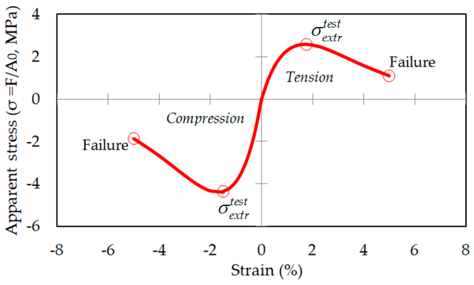
In compression tests of samples, the load F –displacement Δ L plot (Figure 1a) is transformed into the apparent σ ε plot. In this case σ = F / A 0 , and ε = Δ L / L 0 , where A 0 and L 0 are the initial cross-sectional area of the sample, and the initial length (height) of the sample, respectively. Since A 0 and L 0 do not depend on the force F , the load–displacement and stress–strain patterns are analogous [16] (Figure 1). A typical “apparent stress–train” plot (e.g., [12,13]) is schematically shown in Figure 2; usually the compression stress extremum (in absolute value) is about 1.7 times higher than the tensile stress extremum [17]. Relationships between the apparent stress–strain and effective stress–strain are discussed in more detail below, in separate subsections.

1.3. The Problem of Consistency between Plots of Load–Displacement and Apparent Stress–Strain

There is a problem of consistency of the load–displacement relationship’s dependence with the stress–strain relationship; this problem is initiated by the following observations, interpretations, and assumptions.
Hollister et al. [17] showed that there is a large variation in stresses and deformations at the level of bone structural units (i.e., at the tissue level) compared to the corresponding values at the macro level calculated using the continuous bone model. Since bone cells regenerate [18], one of the reasons for the large variation in stress and strain into structural units may be the differences in the age of these cells and, therefore, in the strength of structural units. It can be assumed that even a relatively small load will lead to the next chain of logically related events: The weakest structural units of bone tissue are damaged; as a result, the cross-sectional area decreases, and, accordingly, the average stress in the remaining structural units increases; and an increase in stresses in the material of undisturbed components of bone tissue leads to a corresponding increase in their deformations and probable damage (with insufficient strength).
The above events chain is sufficient to explain the plots’ non-linearity of load–displacement and stress–strain (Figure 1 and Figure 2). Modern testing machines allow us to detect this non-linearity [12,13]. Since the load–displacement relationship for a bone or bone sample is obtained by direct measurements using sufficiently accurate testing machines, the reliability of the data is guaranteed. However, when looking at the plot “apparent stress–strain” (Figure 2), the question arises: Why does the sample not collapse at extreme apparent stress, but collapses when the apparent stress decreases, that is, on the descending plots branch? From a physical point of view, it is logical to assume that the strength of the material of structural units does not decrease under load, passing the point of extremum, at least to the point of inflection of the load–displacement plot (at this point, the second derivative is zero). Then, in accordance with the concept of fracture mechanics, it is logical to assume that as the load increases, part of the material is destroyed and the effective cross-sectional area decreases. In this connection, the question of appropriate quantitative estimates is being updated. The search and justification of the answer to this question is the main task of our research.
As noted above, the load–displacement relationship for a bone sample or a whole bone (Figure 1) is obtained by direct measurements using test machines, so data’s reliability is ensured. However, the stress–strain relationship for the material that the sample consists of is obtained using indirect measurements, so these results may contain errors. The method of indirect measurements and algorithms for estimating the errors of such measurements are given in the article [21]. From the point of view of the theory of indirect measurements [21], within the framework of the given work the following problem appears. We want to know the amount of stress in the material of the structural units of the bone. This stress is difficult or impossible to measure directly. To indirectly estimate the value of the stress, we need to know the relationship between the stress and the directly measured values D 0 and the initial area A 0 , the displacement Δ L , and the force F (Figure 1). Then, using this dependence, it is necessary to develop a computational model that allows us to determine the effective stresses in the material of the structural units and the effective modulus of elasticity for the material of the structural elements (for example, trabeculae [22]). From a practical point of view, it is desirable that the mentioned model does not require an excessively large amount of initial data. Therefore, we measure, find, and experimentally determine some values and, using a computational model, get the desired estimates of the effective stresses and the effective modulus of elasticity of the structural unit of bone tissue’s material. This computational model was obtained in this paper using the methodology of mathematical modeling and new ideas of fracture mechanics. From a practical point of view, it is desirable that the mentioned model does not require an excessively large amount of initial data. Thus, the logic of continuing the study is as follows: we measure D 0 and find A 0 , experimentally determine some values Δ L , and, using a computational model, the desired estimates of the effective stresses and the effective elasticity modulus of the material of the structural units are obtained.

2. Residual Resource Function, Damage Function, and Effective Elasticity Modulus

2.1. Bone as a Biomechanical System of Interacting Structural Units

The feasibility of an approach to the analysis of the load–displacement ratio based on the use of quantized fracture mechanic is well-known from literature studies at the level of the structural units of bone tissue [18,19,20,22] (QFM [23]; note by Pugno [24]: the term is “quantized”—as introduced by Novozhilov [25]—not “quantum”, that could be erratically linked to quantum mechanics). This term was transformed into the name of Finite Fracture Mechanics (FFM) [26]. In other words, we take into account the discontinuous nature of the bone material. When using this approach, the material of the any separate structural unit can be considered linearly elastic, which corresponds to previous studies’ results of osteons [19] and trabeculae [20,22]. In addition, the stresses of the material of the structural unit can be considered at the level of our model as effective stresses. Other important features of modeling the evolution of bone damage and destruction are explained below, in Section 3.4, etc.
Within the framework of this work, it is appropriate to note that since the porous bone material contains mineralized components [6,18], and therefore shows the properties of a brittle or quasi-brittle material, some other porous mineral materials exhibit similar load–displacement patterns in compression tests. For example, the load–displacement curves for uniaxial concrete compression [27,28] are similar to the patterns in Figure 1. This means that the models of damage and destruction of concrete and other brittle materials [29] can be adapted to analyze the evolution of bone tissue damage. Baldonedo et al. [30] draw attention to this possibility. In turn, models of the evolution of damage and destruction of the trabecular bone can be adapted to the analysis of the behavior of bone-like materials [31]. Note that the class of such materials is quite large; however, our study considers only those materials for which there is an extremum on the experimental load–displacement plot.
The main questions of our study include the question noted above: Why does the destruction of bone samples occur on the descending branch of the load–displacement curve? The answer to this question is predictable: because the effective stresses in the material of structural units exceed their strength. However, another question remains open: How are the load–displacement, apparent stress–strain, and effective stress–strain dependencies related? To answer this question, we need a corresponding computational model, an acceptable version of which could not be found in the review [4] or in other articles [12,13,19,30,31,32,33]. The answers to these questions are presented below.

2.2. Effective Cross-Sectional Area and Residual Resource Function

Consider the behavior of a cylindrical sample under uniaxial compression (Figure 1a). Let L 0 and A 0 be the initial length and initial cross-sectional area of the sample, respectively. Under load F , the sample is deformed and internal forces arise in the material of the structural elements of the sample. If the internal forces are large enough, then the weakest structural units of the bone are destroyed first. As a result, the effective cross-sectional area of the sample decreases, the load is redistributed to the undisturbed structural units, and the average stress in the material of these structural units will increase. We denote: A ˜ D as the area of the damaged part of the cross-section of the sample, 0 < A ˜ D A 0 ; and A ˜ = A 0 A ˜ D as the effective cross-section area of the sample. For further use, we will write: d A ˜ / d A ˜ D = 1 ; d A ˜ = d A ˜ D . We use the following dimensionless quantities:
Θ = A ˜ / A 0 ,   ε = Δ L / L 0 ,   ε e x t r t e s t = Δ L e x t r t e s t / L 0 ,   ξ =   Δ L / Δ L e x t r t e s t =   ε / ε e x t r t e s t ,   ω = w / w e x t r t e s t = ( ε / ε e x t r t e s t ) 2 .
The values Δ L e x t r t e s t are determined experimentally and are a constant value in the framework of solving a specific problem; w represents the elastic potential energy of a unit of volume:
w = σ ˜ ε 2 = σ ˜ 2 2 E ˜ = ε 2 E ˜ 2 .
Here σ ˜ and E ˜ are the effective stress and the effective modulus of elasticity, respectively (discussed in more detail below).
The value ω specified in (1) does not depend on which modulus of elasticity is used in the relations (2)—effective E ˜ or apparent E . Based on the physical meaning of the problem, we assume that the effective area A ˜ is partially damaged with an increase of Δ L and, as a result, decreases by d   A ˜ . From a physical point of view, it is logical to assume that the value d   A ˜ is proportional to the change in the strain energy W = ω   A ˜   d ξ (here the value determines the elementary volume):
d A ˜ =   ξ 2 A ˜   d ξ     =     ( ε ε e x t r t e s t ) 2 ( A ˜   d ( ε ε e x t r t e s t ) ) .
Using Θ = A ˜ / A 0 (1), we rewrite Equation (3) in dimensionless form (4):
d Θ Θ   = ξ 2 d ξ .
Integrating both parts of Equation (4) and taking into account that if ξ = 0 , then there are no damaged structural units, i.e., if A ˜ = A 0 , we find Θ ( ξ ) . Then, using the notation (1), we determine the effective area:
A ˜ = A 0   e   1 3   ( ε ε e x t r t e s t ) 3 .
Note to the signs rule: force, displacement, strain, and compression stress are assigned a minus sign; a plus sign is assigned for tension. In Formula (5), s i g n   ( ε ) = s i g n   ( ε e x t r t e s t ) , thus, under tension and compression, the result will be the same. However, the compressive strength of brittle materials is greater than the tensile strength, indicating a possible difference in the effective area under tension and compression in future studies.
From the relation (5), it follows that the function Θ = A ˜ / A 0 (1) introduced above is a function of the residual resource (6):
Θ = e   1 3   ( ε ε e x t r t e s t ) 3 .
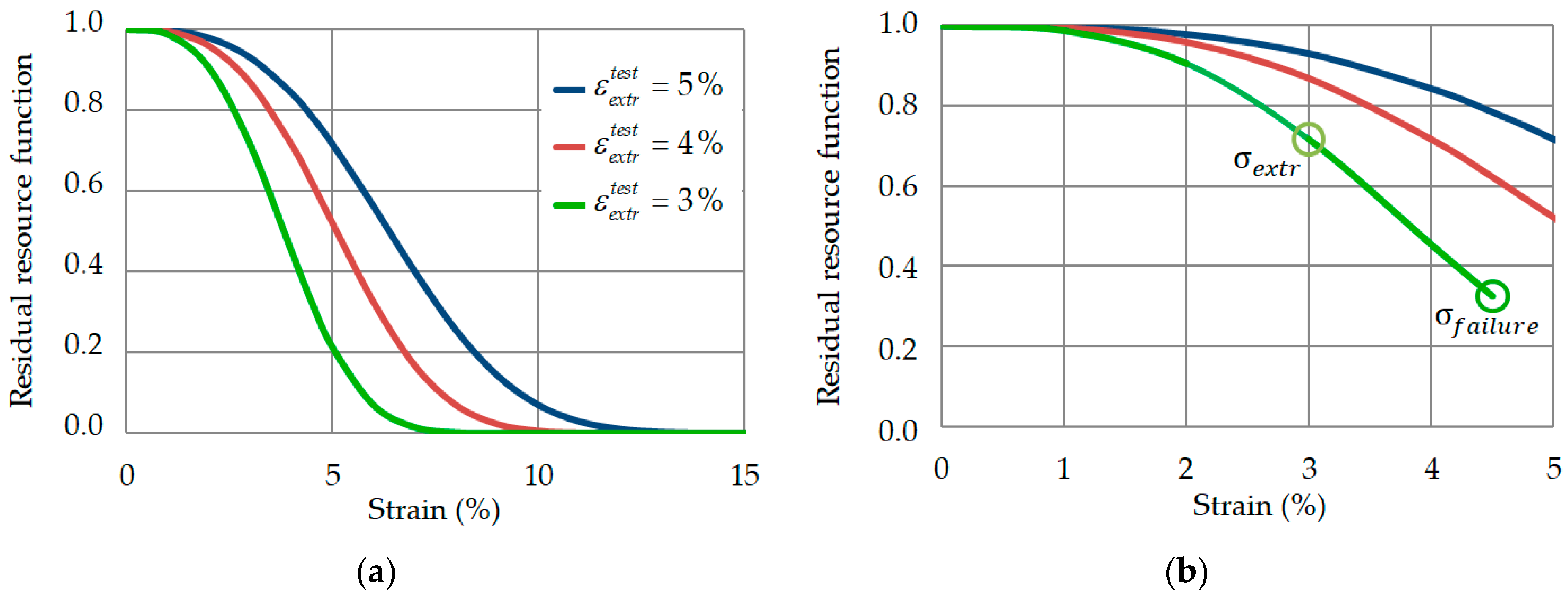
The residual life function (6) varies in the range from 1 to 0; if there are no defects or damage, then Θ = 1 ; if the material is completely degraded, then Θ = 0 . For example, if ε = ε e x t r t e s t , then the remaining resource is Θ = 72 % and, accordingly, 28% of the cross-sectional area is damaged. Function (6) is shown graphically in Figure 3.

2.3. Damage Function

The damage is estimated by the proportion of voids and gaps (if there are cracks) in the cross-section. The degradation of the material is accompanied by an increase in voids; voids are considered as defects in the material. Using function (6), we define the damage function as D = 1 Θ :
D = 1 e   1 3   ( ε ε e x t r t e s t ) 3 .
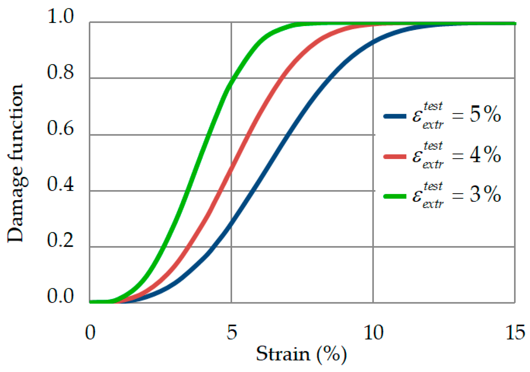
Function (7) is shown graphically in Figure 4. If ε = ε e x t r t e s t , then 28% of the cross-sectional area is damaged.
Alternative approaches are known to determine the damage function, which varies from 0 to 1; D = 0 corresponds to an intact (undamaged) material and D = 1 corresponds to a material in a completely damaged state. A review of the models known in this field has shown that the evolution of damage can be described using the well-known functions of the sigmoid class. Sigmoid functions, whose plots are “S-shaped”, appear in a variety of contexts [34]. For example, in order to model the evolution of damage to a brittle material, in [35] it is proposed to use the logistic function D = 1 / ( 1 + e a r ε ) a r ε , where ε is strain variable, and a and r are the fitting parameters.
Note that when using the known sigmoid functions, the problem arises of fitting the parameters of these functions (including the logistic function) to the modeled damage process. The physical meaning of these parameters is not always clearly defined. The number of parameters may be redundant. In our case, the adjustment of the parameters is not required, since the damage function D = 1 Θ (Figure 4) is obtained using a new function of the residual resource Θ (6), which depends only on the deformation and is justified using the energy criterion in the relations (1)–(7).

2.4. Effective Elasticity Modulus: Substantiation of Model Relationships

According to Hooke’s law, the effective stress σ ˜ and the effective modulus of elasticity E ˜ are related as σ ˜ = ε E ˜ . Here, σ ˜ = F / A ˜ , ε = Δ L / L 0 , and, F = ( Δ L / L 0 ) E ˜ A ˜ . Hence, we express E ˜ , taking into account the relation (5) and the notation (1):
E ˜   = L 0 Δ L F A 0   e   1 3   ( Δ L Δ L e x t r t e s t ) 3 .
The effective modulus of elasticity (8) is determined using the results of standard compression tests.
Equation (8) must correspond to the coordinates Δ L and F of any point on the experimental load–displacement plot. Let Δ L = Δ L e x t r t e s t and F = F e x t r t e s t . Then:
E ˜   = L 0 Δ L e x t r t e s t F e x t r t e s t A 0   e   1 3 .
The relations (8) and (9) can be transformed to form (10) and (11), respectively:
E ˜   = σ ε e   1 3   ( ε ε e x t r t e s t ) 3 .
E ˜   = σ e x t r t e s t ε e x t r t e s t e   1 3 .
Here, σ = F / A 0   and σ e x t r t e s t = F e x t r t e s t / A 0   are the apparent stress, defined experimentally.
We denote E s e c = σ / ε as the secant modulus of elasticity and rewrite (10) as:
E ˜   = E s e c e   1 3   ( ε ε e x t r t e s t ) 3 .
If ε = ε e x t r t e s t , then instead of (12), we can write:
E ˜   = E s e c . e x t r e   1 3 .
Using (13), we define the apparent modulus of elasticity as E s e c . e x t r = E ˜ e 1 / 3 . We accept the hypothesis that the apparent and effective elastic modulus are related by a similar relation. Then, in the general case, you can write:
E   = E ˜ e     1 3 .
An alternative way is known [36] to obtain the relation between the effective and the apparent modulus of elasticity, according to which E ˜ = E s e c . e x t r e 2.718 is not consistent with the obtained result (13). Explaining the almost twofold difference, we note that the result E ˜   = E s e c . e x t r e   1 / 3   1.396 (13) is obtained under the assumption that the effective cross-sectional area A ˜ is partially damaged with an increase of Δ L and, as a result, the area A ˜ decreases by an amount of d   A ˜ . In this case, it is assumed that the value d   A ˜ is proportional to the change in energy, as shown in the ratio (3). Thus, it can be declared that the result of (13) was obtained using the energy criterion
At the same time, the result of [36] was obtained using a simplified (strain) approach based on the assumption that the value is proportional only to the strain [27], i.e., the elastic strain energy was ignored, which led to differences in the coefficients 2.718 and 1.396. In this case, the advantage of the energy criterion mentioned above can be explained by analogy with the advantages of the known energy theory of strength compared to the historically first strength theories [37].

2.5. Effective Elasticity Modulus: Validation of Model Computations

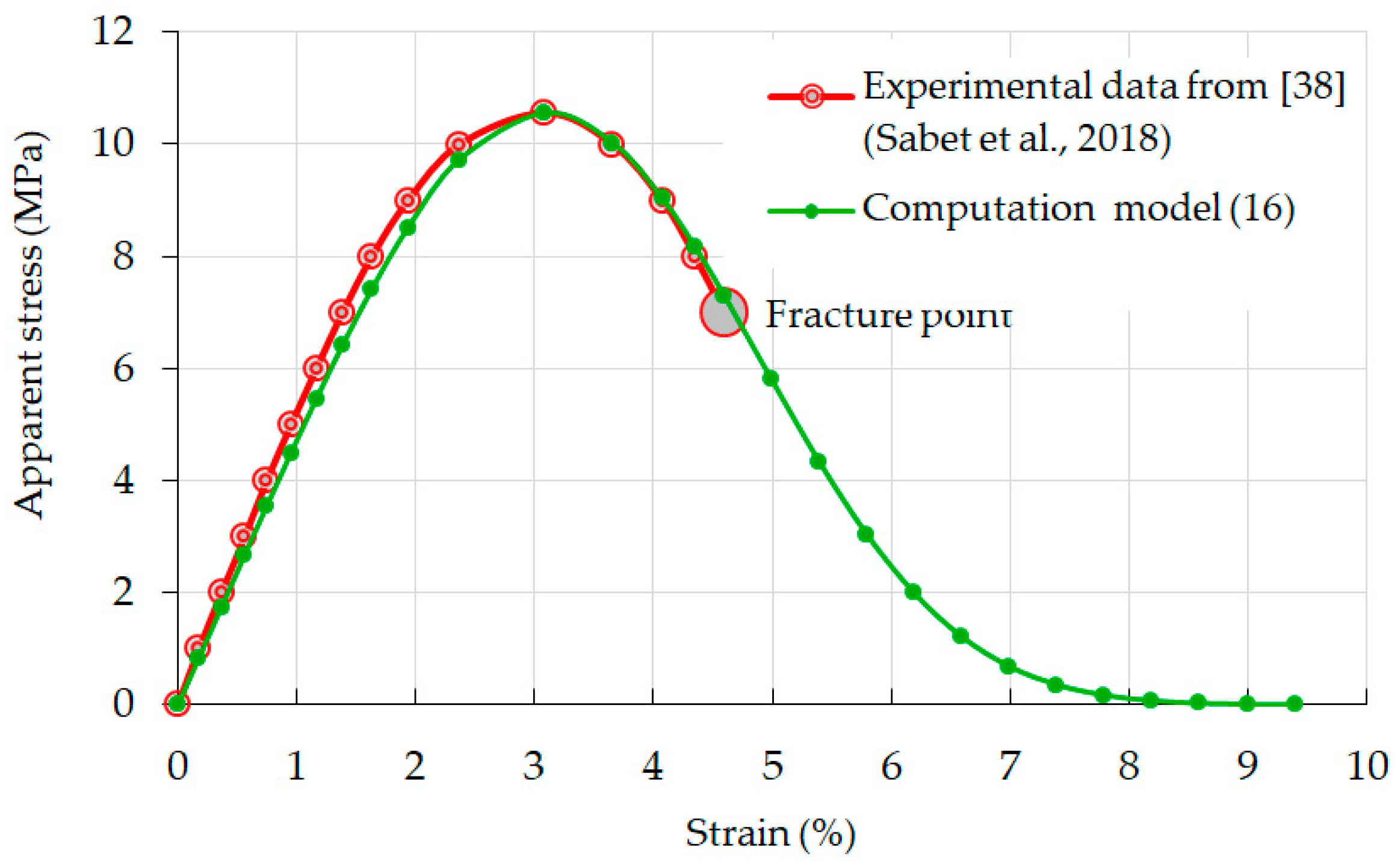
Consider the application of relations (8)–(13) to calculate the effective and apparent modulus of elasticity. As the initial data, we will use the results of compression tests known in the literature by Sabet et al. [38]. In the cited study, the samples of the trabecular bone in the form of cylinders with a height of 8 mm and a diameter of 4 mm were experimentally loaded. We will use the experimental results, which are presented graphically in the article [38]. Adapting the cited results, we write: the apparent modulus of elasticity E = 544   MPa (according to [38], if the volume fraction of the bone is 23.3%); ε e x t r t e s t = 0.031 ;   σ e x t r t e s t = 10.563   MPa (according to Figure 5 of [38]); and E 0.2 = 463   MPa as the apparent modulus of elasticity (for 0.2% apparent yield point according to Figure 5 of [38]).
Using the initial data presented above, we calculate the effective modulus of elasticity (11) as E ˜   = 478   MPa . The resulting value E ˜ differs little from the E 0.2 = 463   MPa mentioned above.
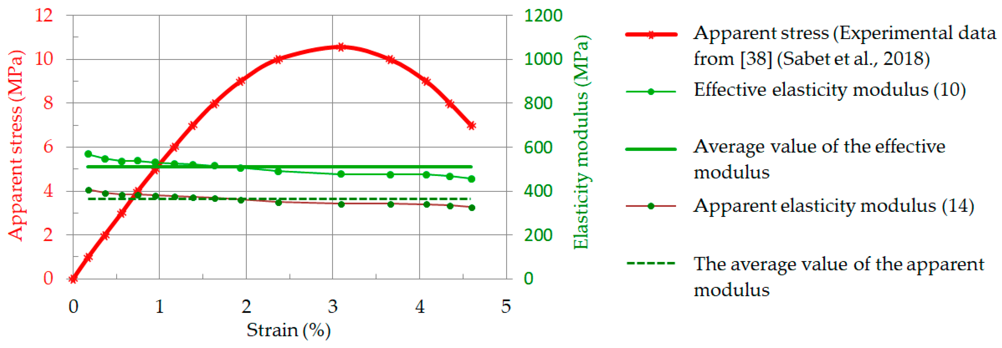
Calculations using Formula (10) showed that the values of both the effective and apparent (14) modulus of elasticity depend on the strain and differ from the average values by ± 10.8 % (Figure 5).
Computational modeling (Figure 5) showed that the values of the effective and apparent elastic modulus are in the range of (458; 569) MPa and (341; 407) MPa, respectively. Accordingly, the average values of the effective and apparent elastic modulus are 365 and 509 MPa. There is a deviation from the average value of ± 10.8 % . This deviation is a quantitative estimate of the dependence of the elastic modulus on deformations. The variations are relatively small, so the proposed computational model can be useful in applied research. It is noteworthy that as the strain increases in the specified interval, the value of the elastic modulus decreases (Figure 5). A similar tendency to change the elastic modulus was recorded in [39].
The adequacy of the model (1)–(14) is confirmed by the consistency with the experimental data of Turunen et al. [22], in which the values of the apparent modulus of elasticity of the trabecular bone are in the range of (300; 487) MPa (according to Table 3 in the article [22]). Using relation (14), we transform this range of values of the apparent modulus of elasticity into the range of values of the effective modulus of elasticity: (419; 680) MPa.
In addition, the above values do not contradict the known range of values of the elastic modulus (6; 1524) MPa (according to Table 3 in the article [17]). Additional data related to model validations (1)–(14) are discussed below.

3. Results

3.1. Load–Displacement Relationship

The left-hand sides of relations (8) and (9) are the same; equating their right-hand sides, we find the relationship between force F and displacement Δ L :
F = F e x t r t e s t Δ L Δ L e x t r t e s t e   1 3   ( 1   ( Δ L Δ L e x t r t e s t ) 3 ) .
Thus, the nonlinear load–displacement function (15a) is defined using only the results of standard tests for uniaxial loading. The positive values of Δ L , Δ L e x t r t e s t , and F e x t r t e s t correspond to tension; the negative values correspond to compression. Taking into account the signs rule, Equation (15a) can be rewritten as:
F = ± F e x t r t e s t Δ L Δ L e x t r t e s t e   1 3   ( 1   ( Δ L Δ L e x t r t e s t ) 3 ) .
However, for a clearer visual comparison, the tension and compression plots of the samples are usually drawn in the first quarter of the coordinate plane.
To summarize, we note the following. Function (15a) was obtained using a sufficiently universal energy criterion in relation (3), which can lead to good predictive properties of this function. However, this function characterizes the behavior of the sample as a structure and, to a lesser extent, reflects the properties of the material. To better understand the properties of the material, it is necessary to know the dependence of the apparent and effective stresses on the deformation.

3.2. Relationship between Strain and Apparent Stress

Deformations and apparent stresses are defined as ε = Δ L / L 0 , ε e x t r t e s t = Δ L e x t r t e s t / L 0 , σ = F / A 0   , and σ e x t r t e s t = F e x t r t e s t / A 0 , respectively. Dividing both parts of Equation (15a) by the initial cross-sectional area A 0 , we obtain:
σ = σ e x t r t e s t ε ε e x t r t e s t e   1 3   ( 1   ( ε ε e x t r t e s t ) 3 ) .
It is important to note that Equation (16a) does not contain any fitting parameters, and only two results of the standard uniaxial loading tests ( σ e x t r t e s t and ε e x t r t e s t ) are sufficient to construct the function σ = σ ( ε ) .
Since bone tissue contains organic and mineral components, we can predict that the developed models (1)–(16a) can be adapted for studies of concrete, frozen soil [27], rocks, and other brittle materials. The features of other models are studied in [35,40].
An analysis of the literature has shown that the destruction of the trabecular bone and similar materials often corresponds to the neighborhood of the inflection point on the plot of the function (15b) or, equivalently, of the function (16a). In other words, the destruction of such materials often (but not always) occurs if the second derivative of the function is zero. The abscissa of this point is denoted as ε f r a c t u r e . Then, from equation d 2 σ / d ε 2 = 0 we find:
ε = ε f r a c t u r e = 2 ( 2 / 3 ) ε e x t r t e s t 1.587 ε e x t r t e s t .
Substituting (16b) into Equation (16a), we get:
σ = σ f r a c t u r e = σ e x t r t e s t 2 ( 2 / 3 ) e 1 0.584 σ e x t r t e s t .

3.3. Relationship between Strain and Apparent Stress: Validation of Model Computations

Let us compare the results of modeling according to Equation (16a) with the experimental data of compression tests [38] mentioned in Section 2.5.
The initial data for calculations according to Equation (16a) are ε e x t r t e s t = 3.08 % and σ e x t r t e s t = 10.563   MPa (according to Figure 5 of [38]).
Figure 6 shows the comparison of the experimental stress–strain plot [38] and the plot constructed by Equation (16a).
As it can be seen, the model is correct for both the ascending and descending branches of the experimental stress–strain plot.
At the experimental point of failure (Figure 6), ε = 4.59 % and σ = 7.00   MPa . The theoretical estimates by (16b) and (16c) are ε f r a c t u r e = 4.89 % and σ f r a c t u r e = 6.17   MPa , respectively. The discrepancies between the theoretical and experimental results are 6.5% and 11.9%, respectively.

3.4. Is There a Short-Term Aggregation of Separate Particles of a Destructible Sample at the Final Stage of Compression Tests?

Commenting on Figure 6, it should be noted that if the strain exceeds 7%, then the predicted decrease in apparent stresses to zero is doubtful. Indeed, depending on the characteristics of both the testing equipment and the properties of the test material, it is possible to press, seal, and consolidate some of the particles of the destroyed sample. In this hypothetical case, at the final stage of compression testing, a new material with an increased density, and therefore with increased strength and rigidity, i.e., with an increased modulus of elasticity, actually appears. A distant analogy may be, for example, the aggregation of wood particles in the process of pressing sawdust in the production of fuel briquettes.
In addition, the increase in strength and stiffness in the compression tests of samples of trabecular tissue can be explained by the fact that, due to the regeneration of bone cells, bone structural elements can be differentiated into three groups: the first group of structural elements with new (young) cells that have not yet reached normal strength; the second group of structural elements of normal strength; and the third group of degraded structural elements. It is logical to assume that, as we approach the final stage of compression testing, the weakest structural elements will be destroyed, and the number of fully functioning structural elements will decrease. Accordingly, the proportion of stronger structural elements increases.
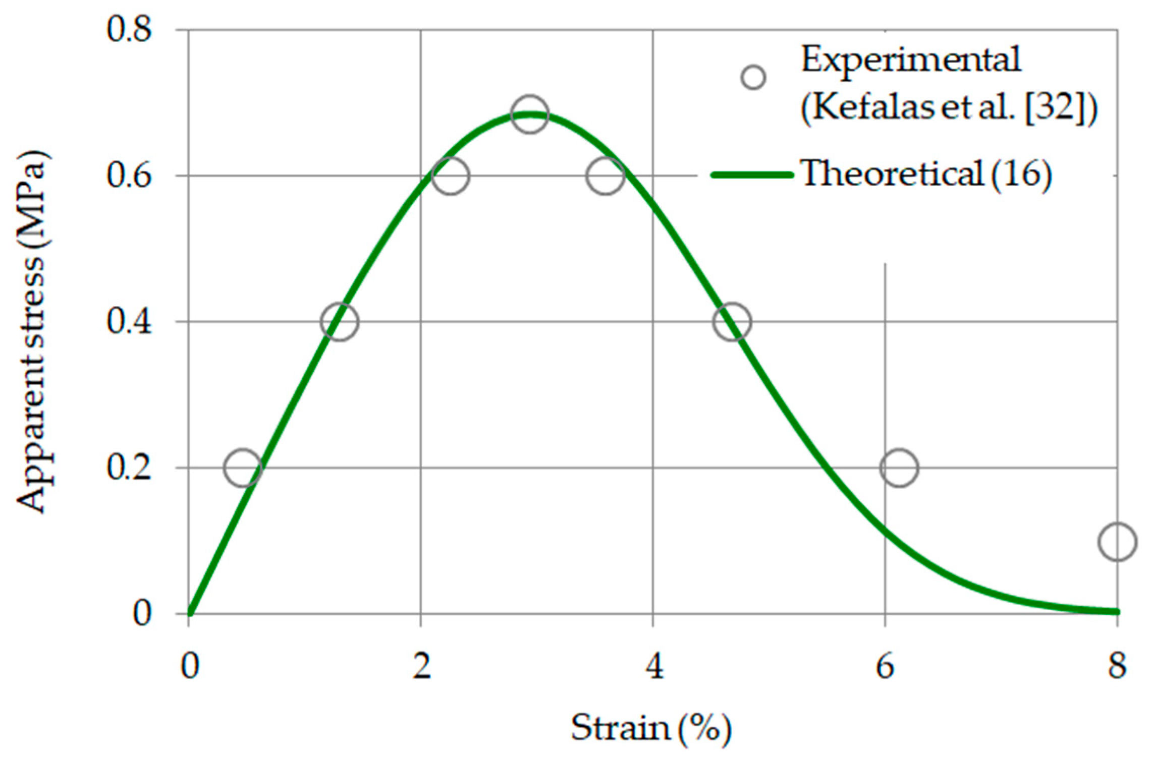
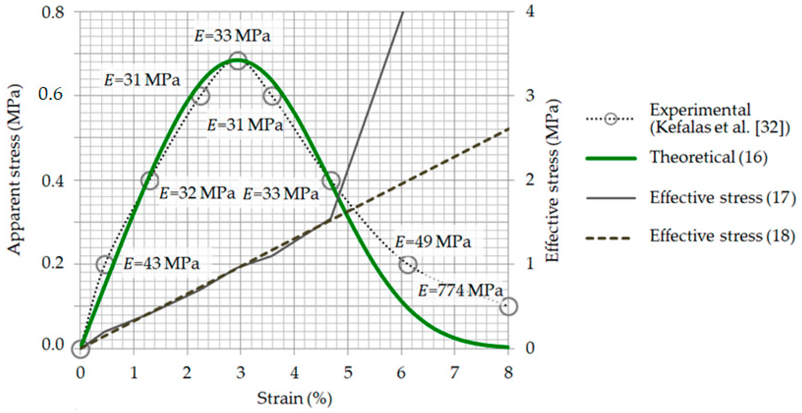
Another feature is that in the compression tests under consideration, only a small fraction of the particles can be consolidated and destroyed again at the final stage of the tests. Therefore, despite the increase in strength noted above, only a small decrease in the rate of reduction of apparent stresses with increasing deformations can be predicted. This means that, at the final stage of the compression tests, the experimental points should be located above the theoretical plot of the function (16a). To test this hypothesis, we use experimental data from Kefalas et al.
Figure 7 shows the results of using Equation (16a) and the experimental data from Kefalas et al. [32]. The apparent stresses (16a) were calculated using the following initial data: σ e x t r t e s t = 0.685   MPa ; ε e x t r t e s t = 2.933 .
Figure 7 shows that at the final stage of the compression tests, the experimental points are shifted up from the theoretical plot of function (16a). This confirms the assumption formulated above that two processes compete at the final stage of compression testing, namely: the destruction and formation of small particles of the material, and the pressing and consolidation of a certain proportion of these particles. From a physical point of view, the consolidation of particles leads to an increase in density, and, as a result, to an increase in the elastic modulus and strength of the particle conglomerate. However, as noted above, in the compression tests, only a small fraction of the particles can be consolidated and destroyed again. Therefore, only a small decrease in the rate of reduction of the apparent stress with increasing deformations can be considered realistic. As you can see (Figure 7), at the final stage of the compression tests, the experimental points are located above the theoretical plot of the function (16a). This confirms the hypothesis formulated above about the possible consolidation of some particles of the destroyed sample and an increase in the elastic modulus and strength of the conglomerate of these particles at the final stage of the compression tests.
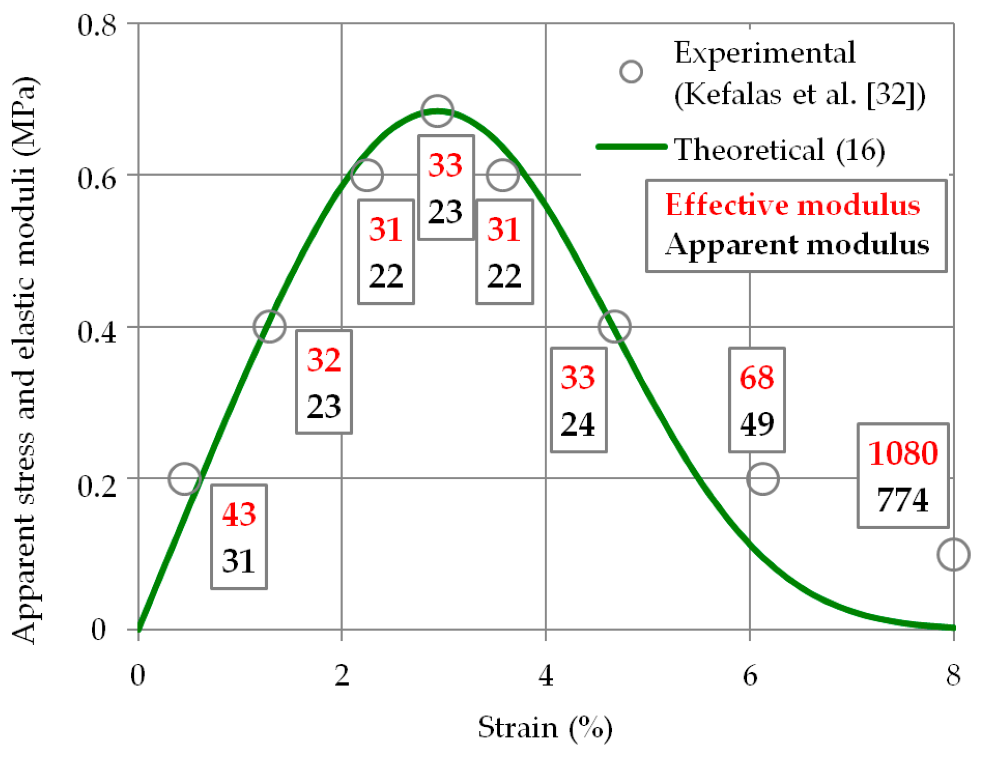
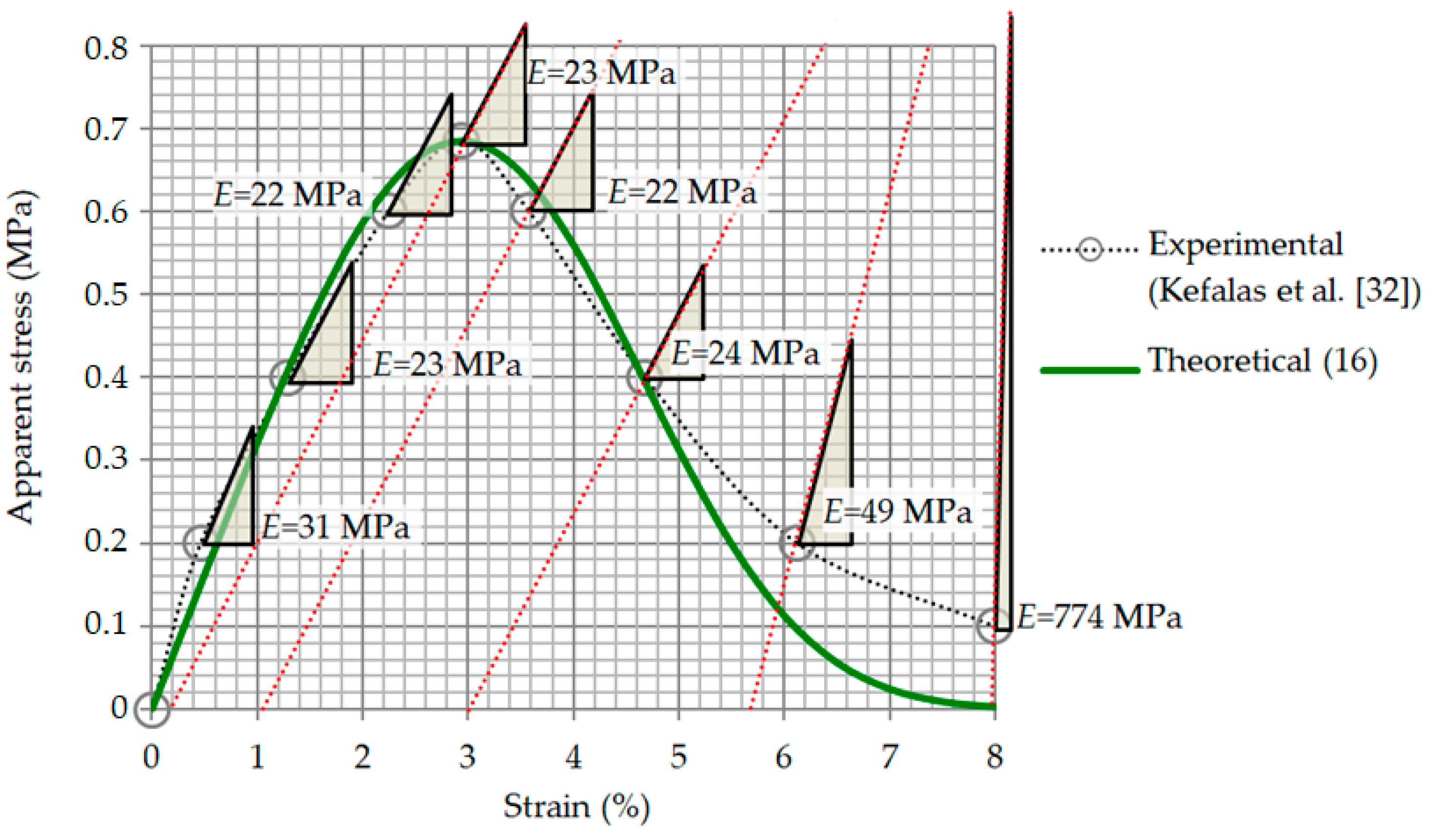
Additional quantitative estimates can be obtained, which probably confirm the above hypothesis about the consolidation of a certain proportion of the particles of the destroyed sample at the final stage of compression tests. The experimental data [32] and the results of the calculations of the effective modulus of elasticity (10) and the apparent modulus of elasticity (14) are given in addition to Figure 7 in Figure 8 and Figure 9. The analysis of the effective stresses given below can improve the understanding of this issue (Figure 10).
As it can be seen (Figure 8 and Figure 9), if the strain does not exceed ~5%, then the model is correct for both the ascending and descending branches of the experimental stress–strain curve. At the final stage of compression tests, when the deformation is equal to or greater than ~5%, the effective modulus of elasticity increases from 33 MPa to 68 MPa. The growth trend of the effective elastic modulus continues with increasing strain and reaches 1080 MPa (Figure 8). Thus, the analysis of the presented data (Figure 8) using the developed models (1)–(16a) confirms the hypothesis formulated above about the consolidation of a certain proportion of particles of the destroyed sample at the final stage of compression tests and, as a result, an increase in the modulus of elasticity and strength of the emerging conglomerate of particles. In addition, Figure 6, Figure 7, Figure 8 and Figure 9 show that the models (1)–(16a) are adequate for the moderate destruction of the sample.
However, the rapid growth of the elastic modulus under large deformations (Figure 8 and Figure 9) should be investigated further, taking into account the characteristics of testing machines and equipment for compression testing.
In order to improve the understanding of the behavior of the trabecular tissue in the tests discussed, it is advisable, in addition to the characteristics discussed above, to consider the effective stresses and their change as a function of deformation.

3.5. Effective Stress

The effective and apparent stresses are defined as σ ˜ = F / A ˜ and σ = F / A 0 , respectively. Using Formula (5), we obtain the relation between the effective and apparent stress:
σ ˜ = σ e   1 3   ( ε ε e x t r t e s t ) 3 .
Substituting (16a) in (17), we transform (17) to the form (18):
σ ˜ = ε σ e x t r t e s t ε e x t r t e s t e   1 3   1.396   σ e x t r t e s t ε e x t r t e s t   ε .
The values σ e x t r t e s t and ε e x t r t e s t are constants within the framework of solving a specific problem. The effective stresses σ ˜ (18) are linearly related to the strain ε .
Figure 10 shows the plots of the theoretical and experimental values of the effective and apparent stress, and the values of the apparent modulus of elasticity are indicated. It can be seen that if the strain exceeds 4.7%, the apparent modulus of elasticity increases and the effective stresses also grow. According to (14), the effective modulus of elasticity also increases, as shown in Figure 8 above. All calculations for plotting in Figure 10 were performed using experimental data from the paper by Kefalas et al. [32].
It should be noted that at the extremum point (Figure 10) ε e x t r t e s t = 2.933 % ;   σ e x t r t e s t = 0.685   MPa , and using the Formulas (16b) and (16c), we obtain the coordinates of the inflection point: ε f r a c t u r e = 4.65 % ; σ f r a c t u r e = 0.400   MPa . It is at this point that the growth of the elastic modulus begins (Figure 9 and Figure 10).
If the strain is 6.12%, then the effective stress is 4.15 MPa; if the strain is 8.00%, then the effective stress is 86.4 MPa (these points are not shown in Figure 10).
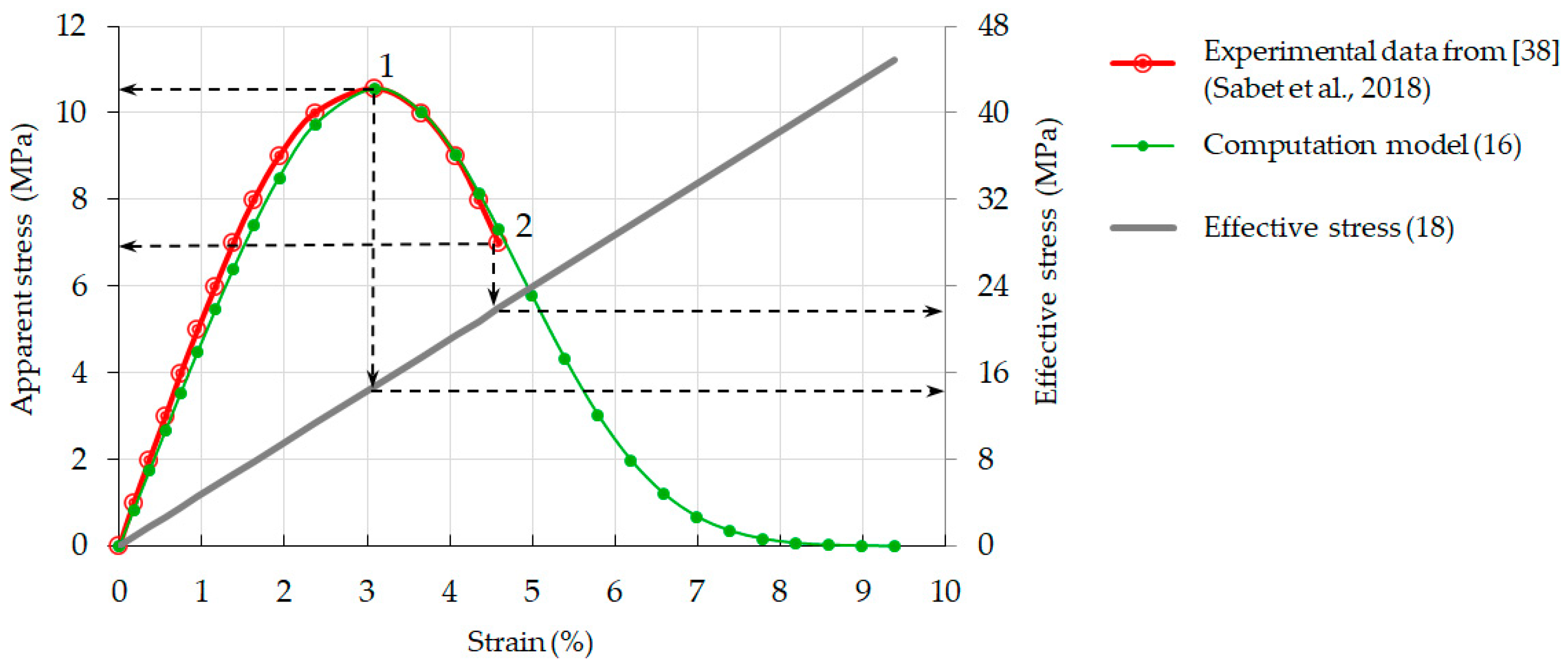
Consider another example. The plots of the effective and apparent stresses (16a) and (18) for the example from Section 3.3 (Figure 6) are shown in Figure 11.
As it can be seen, at the extremum point 1 (Figure 11) the apparent stress is σ = 10.53   MPa , the strain is 3.08%, and the effective stress is σ ˜ = 14.74   MPa . At the final point 2: σ = 7.00 , the strain is 4.59%, and σ ˜ = 21.94   MPa . The results obtained answer the question: Why does the failure occur on the descending branch of the load–displacement plot (or, what is the same thing, on the descending branch of the apparent stress–strain plot)?
The answer is predictable: because the effective stresses grow monotonically up to the final point 2. In other words, according to the concept of this work, the material is considered as a certain structure consisting of structural elements. In accordance with the ideas of fracture mechanics [23,24], the stresses appearing in the material of structural elements are called effective stresses. If the effective stresses (18) increase, the weakest structural elements are destroyed first, and the effective cross-sectional area (5) decreases step by step (Figure 3). As a result, the sample approaches the finish point 2 (Figure 11).

4. Discussion

The results presented above are more representative of the behavior of the trabecular tissue during compression and less illustrative to the tension tests. Theoretically, the behavior of the trabecular tissue in tension is modeled according to the same model (1)–(18) as in compression. The difference is in the signs (15b).
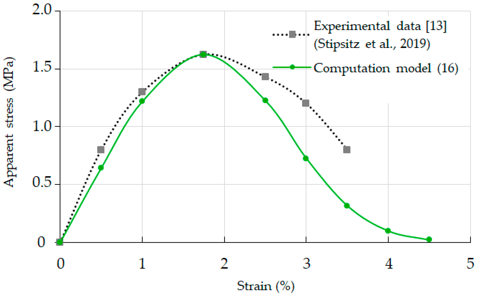
Figure 12 shows a comparison of experimental tensile stresses [13] with the results of calculations using the model (16a).
As can be seen, the model (16a) adequately reflects the trends of growth and decrease of apparent stresses at the stages before and after the point of the stress extremum (Figure 10). However, quantitative estimates of the consistency of the results obtained leave much to be desired, and therefore it is necessary to continue studying the behavior of the trabecular tissue under tensile stress. It can be assumed that the model (1)–(18) is too simple to analyze such a complex object as a trabecular tissue, for which some transformation of the structure is possible [40,41] and changes in the interaction of structural elements during tension. The use of models with parameters [35,42] may be promising both for improving the results of the analysis and for expanding the scope of such models [43].
Nevertheless, for compression, quite adequate results were obtained using the model (1)–(18) (Figure 3, Figure 4, Figure 6, Figure 7, Figure 8, Figure 9, Figure 10, Figure 11 and Figure 12). In addition, using the energy criterion in the ratio (3) and the ideas of fracture mechanics [23,24], the following are justified: the residual resource function (6) and the damage function (7); the formulas for determining the effective elastic modulus using experimental data (8), (10), (11), and the apparent modulus of elasticity (14); the functions of load–displacement (15a) and of apparent stress–strain (16a); and the hypothesis about the consolidation of the particles of the destroyed sample at the final stage of compression tests (Section 3.4).
In addition, in logical connection with the above results, it is shown that the effective stresses increase monotonically up to the destruction of the material (Figure 11). This explains the fracture phenomenon of a brittle material with a decrease in the apparent stress. In other words, it is shown that the failure on the descending branch of the plot force–displacement is a natural consequence of the growth of the effective stresses, and the contradiction in this case is imaginary.

Author Contributions

Conceptualization, G.K. and R.M.; methodology, G.K. and R.M.; validation, R.M.; formal analysis, G.K.; data curation, G.K. and R.M.; writing—original draft preparation, G.K.; writing—review and editing, G.K. and R.M.; project administration, G.K. Both authors have read and agreed to the published version of the manuscript.

Funding

This research received no external funding.

Institutional Review Board Statement

Not applicable.

Informed Consent Statement

Not applicable.

Conflicts of Interest

The authors declare no conflict of interest.

References

  1. Cristofolini, L. In vitro evidence of the structural optimization of the human skeletal bones. J. Biomech. 2015, 48, 787–796. [Google Scholar] [CrossRef]
  2. Yan, C.; Moshage, S.G.; Kersh, M.E. Play During Growth: The Effect of Sports on Bone Adaptation. Curr. Osteoporos. Rep. 2020, 18, 684–695. [Google Scholar] [CrossRef] [PubMed]
  3. Roesler, H. The history of some fundamental concepts in bone biomechanics. J. Biomech. 1987, 20, 1025–1034. [Google Scholar] [CrossRef]
  4. Pahr, D.H.; Reisinger, A.G. A Review on Recent Advances in the Constitutive Modeling of Bone Tissue. Curr. Osteoporos. Rep. 2020, 18, 696–704. [Google Scholar] [CrossRef]
  5. Roux, J.P.; Boutroy, S.; Bouxsein, M.L.; Chapurlat, R.; Wegrzyn, J. Local and global microarchitecture is associated with different features of bone biomechanics. Bone Rep. 2020, 13, 100716. [Google Scholar] [CrossRef] [PubMed]
  6. Wang, X.; Nyman, J.S.; Dong, X.; Leng, H.; Reyes, M. Fundamental biomechanics in bone tissue engineering. Synth. Lect. Tissue Eng. 2010, 2, 1–225. [Google Scholar] [CrossRef]
  7. Fischer, B.; Hofmann, A.; Kurz, S.; Edel, M.; Zajonz, D.; Roth, A.; Schleifenbaum, S. Influence of the fixation technique on the mechanical properties of human cancellous bone of the femoral head. Clin. Biomech. 2021, 82, 105280. [Google Scholar] [CrossRef] [PubMed]
  8. Henkel, J.; Woodruff, M.A.; Epari, D.R.; Steck, R.; Glatt, V.; Dickinson, I.C.; Choong, P.; Schuetz, M.A.; Hutmacher, D.W. Bone regeneration based on tissue engineering conceptions—A 21st century perspective. Bone Res. 2013, 1, 216–248. [Google Scholar] [CrossRef] [Green Version]
  9. Liu, Y.; Luo, D.; Wang, T. Hierarchical structures of bone and bioinspired bone tissue engineering. Small 2016, 12, 4611–4632. [Google Scholar] [CrossRef] [PubMed]
  10. Razi, H.; Predan, J.; Fischer, F.D.; Kolednik, O.; Fratzl, P. Damage tolerance of lamellar bone. Bone 2020, 130, 115102. [Google Scholar] [CrossRef]
  11. Luo, Y. A biomechanical sorting of clinical risk factors affecting osteoporotic hip fracture. Osteoporos. Int. 2016, 27, 423–439. [Google Scholar] [CrossRef]
  12. Schwiedrzik, J.; Gross, T.; Bina, M.; Pretterklieber, M.; Zysset, P.; Pahr, D. Experimental validation of a nonlinear μFE model based on cohesive-frictional plasticity for trabecular bone. Int. J. Numer. Methods Biomed. Eng. 2016, 32, e02739. [Google Scholar] [CrossRef]
  13. Stipsitz, M.; Zysset, P.K.; Pahr, D.H. Efficient materially nonlinear μFE solver for simulations of trabecular bone failure. Biomech. Modeling Mechanobiol. 2019, 19, 861–874. [Google Scholar] [CrossRef] [PubMed] [Green Version]
  14. Zhao, S.; Arnold, M.; Ma, S.; Abel, R.L.; Cobb, J.P.; Hansen, U.; Boughton, O. Standardizing compression testing for measuring the stiffness of human bone. Bone Jt. Res. 2018, 7, 524–538. [Google Scholar] [CrossRef]
  15. Wright, T.M.; Hayes, W.C. Tensile testing of bone over a wide range of strain rates: Effects of strain rate, microstructure and density. Med. Biol. Eng. 1976, 14, 671–680. [Google Scholar] [CrossRef]
  16. Cole, J.H.; van der Meulen, M.C.H. Biomechanics of bone. In Osteoporosis, Contemporary Endocrinology; Leder, B.Z., Wein, M.N., Eds.; Springer: Cham, Switzerland, 2020; pp. 185–209. [Google Scholar] [CrossRef]
  17. Hollister, S.J.; Brennan, J.M.; Kikuchi, N. A homogenization sampling procedure for calculating trabecular bone effective stiffness and tissue level stress. J. Biomech. 1994, 27, 433–444. [Google Scholar] [CrossRef] [Green Version]
  18. Manzini, B.M.; Machado, L.M.R.; Noritomi, P.Y.; da Silva, J.V.L. Advances in Bone tissue engineering: A fundamental review. J. Biosci. 2021, 46, 1–18. [Google Scholar] [CrossRef]
  19. Giner, E.; Arango, C.; Vercher, A.; Fuenmayor, F.J. Numerical modelling of the mechanical behaviour of an osteon with microcracks. J. Mech. Behav. Biomed. Mater. 2014, 37, 109–124. [Google Scholar] [CrossRef] [PubMed] [Green Version]
  20. Wu, D.; Isaksson, P.; Ferguson, S.J.; Persson, C. Young’s modulus of trabecular bone at the tissue level: A review. Acta Biomater. 2018, 78, 1–12. [Google Scholar] [CrossRef] [PubMed]
  21. Ferregut, C.; Nazarian, S.; Vennalaganti, K.; Chang, C.C.; Kreinovich, V. Fast error estimates for indirect measurements: Applications to pavement engineering. Reliab. Comput. 1996, 2, 219–228. [Google Scholar] [CrossRef] [Green Version]
  22. Turunen, M.J.; Le Cann, S.; Tudisco, E.; Lovric, G.; Patera, A.; Hall, S.A.; Isaksson, H. Sub-trabecular strain evolution in human trabecular bone. Sci. Rep. 2020, 10, 13788. [Google Scholar] [CrossRef]
  23. Pugno, N.M.; Ruoff, R.S. Quantized fracture mechanics. Philos. Mag. 2004, 84, 2829–2845. [Google Scholar] [CrossRef] [Green Version]
  24. Pugno, N.M. Dynamic quantized fracture mechanics. Int. J. Fract. 2006, 140, 159–168. [Google Scholar] [CrossRef] [Green Version]
  25. Novozhilov, V.V. On a necessary and sufficient criterion for brittle strength. Prik. Mat. Mek. 1969, 33, 212–222. [Google Scholar] [CrossRef]
  26. Cornetti, P.; Pugno, N.; Carpinteri, A.; Taylor, D. A Coupled Stress and Energy Criterion within Finite Fracture Mechanics. In Fracture of Nano and Engineering Materials and Structures; Gdoutos, E.E., Ed.; Springer: Dordrecht, The Netherlands, 2006; pp. 1107–1108. [Google Scholar] [CrossRef] [Green Version]
  27. Kolesnikov, G. Analysis of Concrete Failure on the Descending Branch of the Load-Displacement Curve. Crystals 2020, 10, 921. [Google Scholar] [CrossRef]
  28. Lv, J.; Zhou, T.; Du, Q.; Li, K.; Sun, K. Evaluation of Stress–Strain Behavior of Self-Compacting Rubber Lightweight Aggregate Concrete under Uniaxial Compression Loading. Materials 2019, 12, 4064. [Google Scholar] [CrossRef] [Green Version]
  29. Mudunuru, M.K.; Panda, N.; Karra, S.; Srinivasan, G.; Chau, V.T.; Rougier, E.; Hunter, A.; Viswanathan, H.S. Surrogate Models for Estimating Failure in Brittle and Quasi-Brittle Materials. Appl. Sci. 2019, 9, 2706. [Google Scholar] [CrossRef] [Green Version]
  30. Baldonedo, J.; Fernández, J.R.; López-Campos, J.A.; Segade, A. Analysis of Damage Models for Cortical Bone. Appl. Sci. 2019, 9, 2710. [Google Scholar] [CrossRef] [Green Version]
  31. Gao, H. Application of fracture mechanics concepts to hierarchical biomechanics of bone and bone-like materials. Int. J. Fract. 2006, 138, 101–137. [Google Scholar] [CrossRef]
  32. Kefalas, V.; Eftaxiopoulos, D.A. Experimental study of cancellous bone under large strains and a constitutive probabilistic model. J. Mech. Behav. Biomed. Mater. 2012, 6, 41–52. [Google Scholar] [CrossRef]
  33. Ural, A. Advanced Modeling Methods—Applications to Bone Fracture Mechanics. Curr. Osteoporos. Rep. 2020, 18, 568–576. [Google Scholar] [CrossRef]
  34. Menon, A.; Mehrotra, K.; Mohan, C.K.; Ranka, S. Characterization of a class of sigmoid functions with applications to neural networks. Neural Netw. 1996, 9, 819–835. [Google Scholar] [CrossRef] [Green Version]
  35. Liu, D.; He, M.; Cai, M. A damage model for modeling the complete stress–strain relations of brittle rocks under uniaxial compression. Int. J. Damage Mech. 2018, 27, 1000–1019. [Google Scholar] [CrossRef]
  36. Baldwin, R.; North, M.A. Stress-strain curves of concrete at high temperature—A review. Fire Saf. Sci. 1969, 785, 1. Available online: http://www.iafss.org/publications/frn/785/-1/view/frn_785.pdf (accessed on 11 March 2021).
  37. Yu, M.H. Advances in strength theories for materials under complex stress state in the 20th century. Appl. Mech. Rev. 2002, 55, 169–218. [Google Scholar] [CrossRef]
  38. Sabet, F.; Jin, O.; Koric, S.; Jasiuk, I. Nonlinear micro-CT based FE modeling of trabecular bone—Sensitivity of apparent response to tissue constitutive law and bone volume fraction. Int. J. Numer. Methods Biomed. Eng. 2018, 34, e2941. [Google Scholar] [CrossRef] [PubMed]
  39. Aerens, R.; Vorkov, V.; Duflou, J.R. Springback prediction and elasticity modulus variation. Procedia Manuf. 2019, 29, 185–192. [Google Scholar] [CrossRef]
  40. Buccino, F.; Colombo, C.; Vergani, L.M. A Review on Multiscale Bone Damage: From the Clinical to the Research Perspective. Materials 2021, 14, 1240. [Google Scholar] [CrossRef] [PubMed]
  41. Kim, T.-H.; Lee, D.-Y.; Jung, S.-K. Comparison of Trabecular Bone Mineral Density Measurement Using Hounsfield Unit and Trabecular Microstructure in Orthodontic Patients Using Cone-Beam Computed Tomography. Appl. Sci. 2021, 11, 1028. [Google Scholar] [CrossRef]
  42. Stojković, N.; Perić, D.; Stojić, D.; Marković, N. New stress-strain model for concrete at high temperatures. Teh. Vjesn. 2017, 24, 863–868. [Google Scholar] [CrossRef] [Green Version]
  43. Khoroshilov, K.V.; Katarov, V.K.; Gavrilov, T.A.; Kolesnikov, G.N. Strength and Elastic Modulus of Frozen Sandy Soil as a Material for a Logging Road. Resour. Technol. 2019, 16, 33–43. [Google Scholar] [CrossRef]
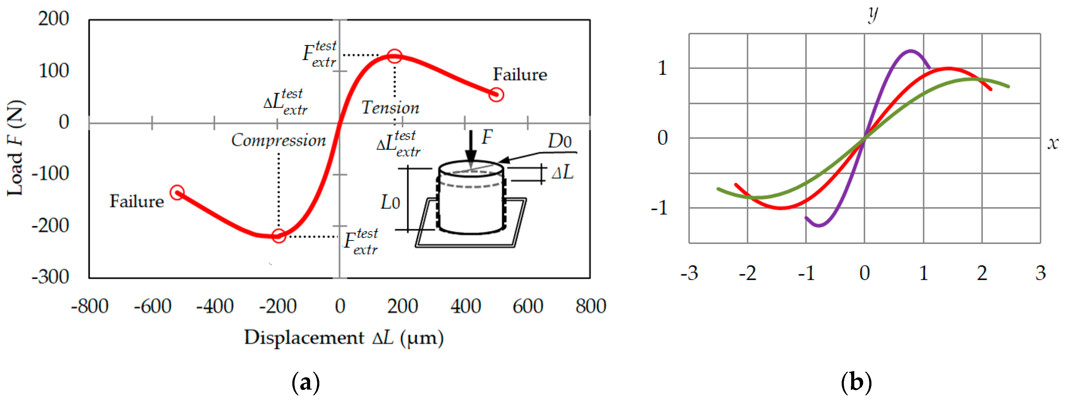
Figure 1. (a) Typical uniaxial load-displacement plots. Tension and compression asymmetry is visible; (b) Function plots y = A sin ( k x ) for different values A and k on limited intervals of the variable x .
Symmetry 13 01051 g001
Figure 2. A typical plot of apparent stress versus strain is similar to a load-displacement plot. Only the scale changes along the abscissa and ordinate axes. Strain is defined as ( Δ L / L 0 ) · 100 % .
Symmetry 13 01051 g002
Figure 3. Residual resource function Θ = Θ ( ε ) : (a) 0   <   ε 0.15 ; (b) 0   <   ε 0.05 ; at the final stage ( σ = σ f a i l u r e ), the residual resource is 32% (68% of the cross-sectional area is damaged).
Symmetry 13 01051 g003
Figure 4. Damage function (7).
Symmetry 13 01051 g004
Figure 5. Apparent stress, effective elasticity modulus, and apparent elasticity modulus.
Symmetry 13 01051 g005
Figure 6. Apparent stress, effective modulus of elasticity, and apparent modulus of elasticity.
Symmetry 13 01051 g006
Figure 7. Apparent stress: theoretical (16a) and experimental [32].
Symmetry 13 01051 g007
Figure 8. Apparent stress, effective and apparent elastic moduli.
Symmetry 13 01051 g008
Figure 9. Apparent stress and apparent modulus of elasticity. As it can be seen, at the extremum point, the elastic modulus E E 0.2 .
Symmetry 13 01051 g009
Figure 10. Apparent and effective stress and the apparent modulus of elasticity. It can be seen that an increase in the strain and the associated effective stress will lead to the ultimate destruction of the sample or to an emergency stop of the test machine.
Symmetry 13 01051 g010
Figure 11. Apparent and effective stresses.
Symmetry 13 01051 g011
Figure 12. Results of calculations by (16a) and the experimental data for a sample of trabecular tissue under tension.
Symmetry 13 01051 g012
Publisher’s Note: MDPI stays neutral with regard to jurisdictional claims in published maps and institutional affiliations.