Modeling and Trajectory Planning Optimization for the Symmetrical Multiwheeled Omnidirectional Mobile Robot

Abstract

Trajectory optimization is the series of actions that are taken into consideration in order to produce the best path such that it improves the overall performances of physical properties or reduces the consumption of the resources where the restriction system remains maintained. In this paper, first, a compact mathematical model for a symmetrical annular-shaped omnidirectional wheeled mobile robot (SAOWMR) is derived and verified. This general mathematical model provides an opportunity to conduct research, experiments, and comparisons on these omnidirectional mobile robots that have two, three, four, six, or even more omnidirectional wheels without the need to switch models or derive a new model. Then, a new computationally efficient method is proposed to achieve improvements in the trajectory planning optimization (TPO) for a SAOWMR. Moreover, the proposed method has been tested in collision-free navigation by incorporation of the path constraints. Numerical tests and simulations are presented aiming to ensure the efficiency and effectiveness of the proposed method.

1. Introduction

Recently, autonomous mobile robots have been attracting increasing attention due to their extreme importance for daily human life in many applications that include industrial and medical aspects. The type of mobility categorizes the mobile robot into omnidirectional (holonomic) and nonholonomic. Omnidirectional mobile robots (OMRs) have attracted greater attention as a result of maneuvering proficiency; that is, they can modify the direction of motion without needing to utilize midway steps compared with the conventional nonholonomic mobile robots [1]. Although the OWMR is not alone in the field of holonomic mobile robots, it outperforms other OMRs such as the legged robots in ordinary terrain due to its energy efficiency and low complexity [2,3].

Omnidirectional wheels or what have become known as special wheels are very widespread for OMRs. They were designed to perform active movements in the direction perpendicular to the motor shaft and passive movements in the direction of the motor shaft, providing the mobile robot superior flexibility in an overcrowded environment [4]. The structures of different types of omnidirectional wheels are depicted in Figure 1. J. Grabowiecki proposed for the first time the concept of the omnidirectional wheel [5]. The presented omnidirectional wheel, shown in Figure 1a, involves a central wheel and multiple inner passive small rollers surrounding the diameter of the wheel that can slide in the direction of the motor shaft. Since the axes of these rollers are perpendicular to the axis of the wheel, this omnidirectional wheel design is known as the orthogonal wheel. The practical use of this version of the omnidirectional wheels led to many issues in terms of the platform movement accuracy and stability such as the vibrations and slippage because of the unbalanced contact concerning the wheel and the ground. Great efforts were made by researchers to create modified designs of the omnidirectional wheels in order to achieve superior improvements. In the work described in [6], a Swedish engineer constructed a novel design of an omnidirectional wheel, presented in Figure 1b, called Mecanum wheel, where the passive rollers are mounted on angles in an attempt to achieve continuous contact between the wheel and the ground. The first OWMR with four Mecanum wheels, called URANUS, was assembled in the work described in [7]. Many studies have been presented on the basis of the Mecanum wheels, such as [8,9,10,11,12,13]. The usage advantages and disadvantages of OWMRs with the Mecanum wheels are discussed in [14,15]. The advantages are summarized by the omnidirectional performance that the Mecanum wheel provides, allowing maneuverability and full mobility in an overcrowded environment. Moreover, the Mecanum wheels show better balancing performance compared with the older versions of the omnidirectional wheels. However, the Mecanum wheels have also some weaknesses. A vehicle with Mecanum wheels is subject to slippage. This slippage is challenging to calculate and model. Furthermore, the gap between any two adjacent rollers causes vertical and horizontal vibrations in the moving platform, which evidently affect the accuracy and the stability of the mobile robots. The concept of the dual overlapping parallel omnidirectional wheel, depicted in Figure 1c, was patented in [16] as a modified version of the conventional orthogonal wheel aiming to improve the stability and accuracy of OWMRs. This dual omnidirectional wheel has achieved great popularity in both commercial and academic aspects; more than 500 studies have cited and utilized this model. In [17], another enhanced version of the orthogonal wheel, represented in Figure 1d, that ensures continuous contact between the surface of the wheel and the ground was proposed to achieve stability improvements by minimizing the gaps between the rollers. An alternative special wheel scheme of the omnidirectional wheel, displayed in Figure 1e, is the ball wheel mechanism [18]. It uses two arrays of rollers disposed around two circles and an active ring capable of rotating around an axis through the center of the ball. It has been proven that an OWMR with three such ball wheel mechanisms possesses full mobility.

Another essential matter with regard to determining the number of the special wheels is their distribution on the circumference of the OWMR and the extent of its relationship with mobility performance. With regard to OWMRs with the standard Mecanum wheels, it has been proven that the symmetrical rectangular configuration of four wheels is the optimal configuration [19]. However, three Mecanum wheels distributed evenly on the circular shape platform in order to balance the load could also be used with full mobility performance, as described in [20,21]. Concerning the OWMRs with the orthogonal wheels whose roller axes are tangent to the wheel circumference, the most popular design is the circular array arrangement of three or four wheels. Although OWMRs with three omnidirectional wheels possess complete mobility performance, stability problems could be raised in some cases due to the high center of gravity [22,23]. Incrementing the number of omnidirectional wheels can solve the stability problem [1]. Sometimes the necessity of promoting the carrying and transportation capacity of an OWMR is an important reason to increase the number of omnidirectional wheels [24].

Numerous studies on modeling and controlling OMRs have been published. In [25], the authors presented an algorithm for kinematic feedback control of an OMR with four Mecanum wheels. The method proposed in [26] determines the trajectory of the wheelchair with manual pushrim drive by utilizing differential control based on the kinematic model. The visualization of the wheelchair motion trajectory is done by the use of independent measurements on both left and right drive wheels. The impact of the differential steering of a wheelchair with a pushrim on variations in the position of the body’s center of gravity was investigated in [27] based on the kinematic modeling where the transverse relocation of the measured body’s center of gravity in relation to a point on the wheelchair trajectory was assumed by measuring the wheelchair trajectory and the body’s center of gravity. Kinematics modeling and mobility analyses were proposed in [28,29] regarding OMRs with three orthogonal wheels. In [30], resolved acceleration control method, PID method, fuzzy model method, and stochastic fuzzy servo method were used to develop a feedback control system for OMRs with three orthogonal wheels. The research conducted in [31] presented a motion control method based on an inverse linearized kinematic model. A computationally inexpensive near-optimal trajectory generation and control method was proposed in [32]. The work presented in [33,34] formulated the optimal trajectory generation problem as a near-optimal minimum time trajectory such that the solution is based on a relaxed optimal control problem (OCP).

Various studies conducted in the last few years provided a great amount of novelty and contributions regarding OMRs that utilize special wheels. The authors of [35] proposed a novel kinematics and dynamics modeling of an OMR with four Mecanum wheels by utilizing the principle of virtual work where the control of the actuators is done by the presented dynamic model equations. A novel energy modeling method for mobile robots is proposed in [36], allowing the robots to calculate and predict energy consumption. In the work presented in [37], the inverse and forward kinematics for an OMR with six Mecanum wheels are detailed and simulated. The control method of an OWMR with four omnidirectional wheels proposed in [38] depends on the use of a 32-bit ARM microcontroller so that the kinematic modeling will be utilized as feedback. In the work presented in [39], a model predictive fault-tolerant control (MPFTC) scheme was designed for an OWMR with four Mecanum wheels in order to appropriately exploit the inherited actuation redundancy of the robot. In the work presented in [40], a type-2 fuzzy logic controller was designed for an OWMR in order to control the motor speed of the wheels so that the robot behavior remains maintained. The work presented in [41] solved the trajectory tracking problem on uneven terrain for an OWMR using a double closed-loop control strategy. In [42], proportional derivative control tuning was established for OMRs so that the tracking error and energy consumption could be minimized by the use of the dynamic optimization approach. The authors of [43,44,45,46] designed fuzzy controllers to allow OWMRs to track the desired trajectory. A model predictive control (MPC) algorithm was designed by the authors of [47] in an effort to achieve point stabilization and trajectory generation. The research presented in [48] combined the sliding mode control (SMC) with the backstepping technique in order to control an OWMR with four wheels where the kinematic and dynamic model of the robot was utilized in designing the controller. The coupled sliding mode control (CSMC) method was used in [49] in order to achieve a satisfactory tracking control for an OMR. In [50], the adaptive robust control was proposed for the trajectory tracking of an OMR in the presence of uncertainties. The study presented in [51] used a flatness-based control scheme hardware-in-the-loop simulation platform for an OMR where the control input from the simulation model was reassigned to the robot hardware and the feedback to the simulation model was done by a Kinect-based vision system. The trajectory tracking for an OMR with four omnidirectional wheels presented in [52] was carried out using PID and linear quadratic tracking (LQT)-based controller. In [53], the author utilized a constrained dynamic inversion-based (CDIB) approach that incorporates vehicle dynamics to solve the optimal trajectory generation problem of an OWMR with three orthogonal wheels. A novel control system was proposed in [54] based on mixed reality for the path planning of OWMRs. The research presented in [55] addressed the velocity tracking problem for an OWMR with four Mecanum wheels by utilizing novel voltage-based control law with visual feedback. In [56], the authors proposed using improved ant colony optimization (IACO) to search for the optimal path for an OWMR.

The obstacle avoidance problem has been seriously considered in many studies discussing the trajectory generation of OWMRs. The algorithm proposed in [57] plans a reference path that meets the conditions of obstacle avoidance based on Bézier curves, then the motion planning that satisfies the dynamic constraint is solved as a minimum-time optimal trajectory problem. The problem of optimal trajectory in the presence of static obstacles was formulated in [58] as a constrained nonlinear optimal control problem. However, a direct method of numerical solution was used to solve the problem. Robert et al. in [59] established a hybrid method of obstacle-avoidance motion planning in dynamic environments where a global deliberate approach is applied to determine the motion in the desired path line and a local reactive approach is used for moving obstacle avoidance. In [60], the authors proposed a navigation system for an OWMR with three orthogonal wheels to ensure obstacle avoidance by using an MPC strategy through the path obtained by the potential field method. In [61], vision-based navigation for an industrial OWMR with four Mecanum wheels was proposed, allowing the robot to navigate autonomously and perform anticollision path planning. The research presented in [62] proposed a hybridized approach based on the use of A* algorithm and the fuzzy analytic hierarchy process (FAHP) together with bio-inspired control method in order to achieve optimal path planning and fast control performance in both static and dynamic working environments. In [63], the velocity obstacles (VO) approach was integrated with the nonlinear model predictive control (NMPC) in order to accomplish collision avoidance online in the dynamic environment. The research presented in [64] combined the adaptive controller with type-2 fuzzy logic to achieve trajectory tracking and obstacle avoidance for OMRs. In [65], a fuzzy behavior-based approach for an OMR with three omnidirectional wheels was proposed to track a target while avoiding obstacles along its path. The work presented in [66] proposed using swarm intelligence optimization in order to design appropriate path planning methods in static and dynamic environments.

Navigational characteristics and localization analysis are indispensable aspects of mobile robots research, and many recent studies have contributed to this domain. The research presented in [67] proposed several contributions to the field of indoor localization for ambient assisted living in smart homes, including new methodologies that used multimodal components to detect a user’s indoor location and its spatial coordinates while interpreting the accelerometer and gyroscope data. In [68], human-aware robot navigation was proposed regarding mobile robots in domestic areas, allowing the mobile robot able to navigate according to the user preferences. The research presented in [69] developed a method of vision-based indoor mobile robot navigation in which the visual navigation problem is transferred to scene classification. Furthermore, a shallow convolutional neural network was designed for this purpose; it had high scene classification accuracy and efficiency in processing images captured by a monocular camera. In [70], a multimodal deep learning method was utilized for mobile robot navigation in a static indoor environment. Additionally, a fuzzy-based system was designed in the study to collect the datasets for training the designed multimodal network. In the work presented in [71], probabilistic approaches for multiple mobile robots in indoor and outdoor environments were designed based on sensor fusion, where the extended Kalman filter (EKF) was used to estimate the position and orientation of the robot. In the work presented in [72], an autonomous mobile robot was utilized in the agriculture industry; the robot was able to navigate through occluded crop rows and perform various phenotyping tasks, such as measuring plant volume and canopy height using 2D LiDAR. A new localization method proposed in [73] aimed to address the navigation problem regarding the mobile robot in non-line-of-sight (NLOS) situation. Stereo images obtained by a stereo camera were utilized in [74] to enhance the localization of a mobile robot. In [75], a neural network data fusion approach was presented to enhance the real-time performance and the accuracy of localization for mobile robots in indoor environments by eliminating the effects produced by measurement errors. In the research presented in [76], a light-emitting diode (LED)-based system was designed in order to achieve communication and localization for a mobile robot, and the Kalman filter was used in this system to acquire the prediction of the robot’s position and orientation.

This study aims to derive a compact and complete mathematical model for a symmetrical annular-shaped omnidirectional wheeled mobile robot (SAOWMR) with $n$ omnidirectional wheels. This model will provide an opportunity to conduct research, experiments, and comparisons on the base of SAOWMRs with two, three, four, or even more omnidirectional wheels without the necessity to switch models or derive a new model. Moreover, this research also focuses on developing a new computationally effective method based on the complete model of a SAOWMR with n omnidirectional wheels so that improvements in the trajectory planning optimization (TPO) can be achieved. Another aim of this work is to incorporate path constraints so that the SAOWMR can navigate with a collision-free optimal trajectory.

The rest of this paper is structured as follows: The kinematic and dynamic model of a SAOWMR with multiple wheels is presented in Section 2. In Section 3, a new computationally effective method is developed in order to achieve improvements in solving the optimal control problem regarding a SAOWMR with n omnidirectional wheels. In Section 4, the results obtained by the proposed method are discussed and compared with those produced by the CDIB method to demonstrate the effectiveness of the presented method. The obstacle avoidance navigation process is discussed in Section 5, and the conclusion of this study is presented in Section 6.

2. Mathematical Modeling of a SAOWMR with n-Omnidirectional Wheels

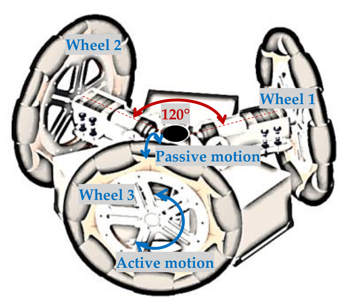
2.1. SAOWMR Description and Topology

A SAOWMR with more than two omnidirectional wheels is an omnidirectional mobile robot that possesses full omnidirectional motion proficiencies as it can move instantaneously in any direction from any configuration. The maneuverability advantage of this robot is based on the usage of the orthogonal omnidirectional wheels that achieve active movements in the direction orthogonal to the motor shaft and passive movements in the direction of the motor shaft, enabling the wheel to move simultaneously in two directions. Although several types and shapes of the orthogonal omnidirectional wheels are available to be implemented, the continuous alternate orthogonal omnidirectional wheels were selected for use in this study to achieve stable performance as they provide continuous trace between the surface of the wheel and the ground. The considered orthogonal wheel consists of a central wheel carrying a number of inner rollers and larger outer rollers arranged alternately surrounding the circumference of the wheel that can slide freely in the direction of the motor shaft. The angle between the roller axis and the central wheel axis is 90°. Figure 2 demonstrates the structure and the configurations of the considered continuous alternate orthogonal omnidirectional wheel.

A SAOWMR includes several omnidirectional wheels distributed regularly around an annular-shaped platform. The holonomicity of motion allowing the robot to rotate and translate independently and simultaneously is determined based on the use of three omnidirectional wheels attached to three independent actuators so that motion with 3 degrees of freedom is achievable. Incrementing the number of omnidirectional wheels can solve some stability problems, as shown in [1]. Moreover, the necessity of promoting the carrying and transportation capacity of the robot is also an important reason to increment the number of omnidirectional wheels [24]. A SAOWMR with only two omnidirectional wheels is still able to move from one configuration to another by breaking up the complex motion into pure rotation and pure translation. The configuration of a SAOWMR with n- omnidirectional wheels distributed around the robot platform where the angle between any two adjacent wheels is φ is depicted in Figure 3. The positive direction of rotation is considered as the rotation in the counter-clockwise direction. Moreover, L is the radius of the SAOWMR.

A SAOWMR possesses clear and interesting symmetrical configurations and topology as its geometric shape can be divided into several identical portions that are organized in a systematized manner. Several types of symmetry can be observed clearly in the case of a SAOWMR, including reflexive, rotational, translational, and scale symmetry. Another interesting symmetrical property that can be detected easily in Figure 4 is that the number of the symmetrical axes of the SAOWMR is equal to the number of its omnidirectional wheels.

Figure 5 shows the real prototype of a SAOWMR with three omnidirectional wheels.

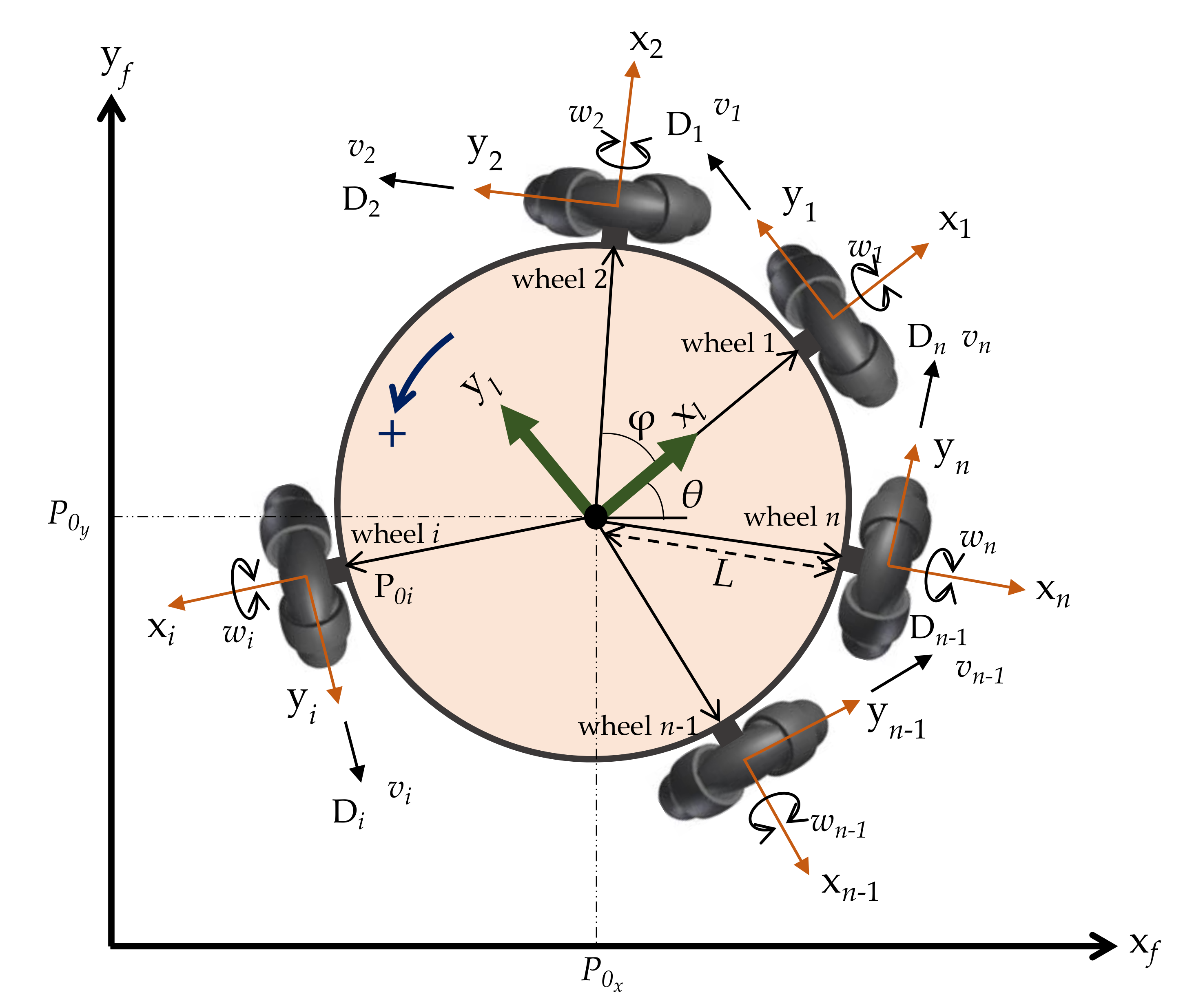
2.2. Geometry of the SAOWMR

The generic configuration of the SAOWMR considered in this study is shown in Figure 6. The structure of the robot includes n omnidirectional orthogonal wheels correspondingly prearranged at $\phi$ degrees on the boundary of the robot platform. In this consideration, the angle$\phi$ depends on the number of the omnidirectional wheels provided, for example, $\phi$ equals 180° if the SAOWMR has two wheels and 90° if the robot possesses four wheels. The omnidirectional wheel and its motor shaft hold the same rotational axle. In this sense, translational velocities $v_1{, v}_2, \cdots {, v}_n$ are applied to the n wheels along the directions ${\mathrm{D}}_1{, \mathrm{D}}_2, \cdots {, \mathrm{D}}_n$, respectively. The angular velocity of the ith wheel shaft is noted as ${\omega }_i$. Hence, the positive direction of rotation is defined to be the rotation in the counter-clockwise direction. A local reference frame $\left({\mathrm{o}}_l{, \mathrm{x}}_l{, \mathrm{y}}_l\right)$ is associated with the center of mass of the robot so that the ${\mathrm{x}}_l$ axis is coincident with the axis of rotation of the first wheel. Another system of n local reference frames is distributed equally to n omnidirectional wheels so that the ${\mathrm{x}}_i$ axis of the frame $\left({\mathrm{o}}_i{, \mathrm{x}}_i{, \mathrm{y}}_i\right)$ corresponds with the rotational shaft of the ith wheel. Moreover, a system of global reference frame $\left({\mathrm{o}}_f{, \mathrm{x}}_f{, \mathrm{y}}_f\right)$ is defined in order to detect the motion of the robot in such a way that the axes ${\mathrm{x}}_l$ and ${\mathrm{x}}_f$ are associated by the angle θ. The radius of the SAOWMR is noted as L. The positional vector of the ith omnidirectional wheel drive is noted as $P_{0i}$. The point $\left(P_{0_x}{,P}_{0_y}\right)$ is the projection of the center of mass of the robot on the global reference frame.

2.3. Kinematic Model of the SAOWMR

The general transformation matrix between the frame attached to the ith wheel and the local reference frame attached to the center of mass of the robot can be given as follows:

$${ }^l{\mathbf{T}}_i=\left[\begin{array}{cccc}\cos \left(\left(i-1\right)\phi \right)& -\sin \left(\left(i-1\right)\phi \right)& 0& L\cos \left(\left(i-1\right)\phi \right)\\ \sin \left(\left(i-1\right)\phi \right)& \cos \left(\left(i-1\right)\phi \right)& 0& L\sin \left(\left(i-1\right)\phi \right)\\ 0& 0& 1& 0\\ 0& 0& 0& 1\end{array}\right]$$

(1)

The positional vector ${\mathrm{P}}_{0i}$ of the ith omnidirectional wheel drive unit is calculated in terms of the local reference frame $\left(o_l{, x}_l{, y}_l\right)$ as

$${ }^l{\mathrm{P}}_{0i}={ }^l{\mathbf{T}}_i\left[\begin{array}{c}0\\ 0\\ 0\\ 1\end{array}\right]=\left[\begin{array}{c}L\cos \left(\left(i-1\right)\phi \right)\\ L\sin \left(\left(i-1\right)\phi \right)\\ 0\\ 1\end{array}\right]$$

(2)

The unit vector ${\mathrm{D}}_i$ that states the direction of the ith motor relative to the local reference frame $\left(o_l{, x}_l{, y}_l\right)$ is given by

$${ }^l{\mathrm{D}}_i={ }^l{\mathbf{R}}_i\left[\begin{array}{c}0\\ 1\\ 0\end{array}\right]=\left[\begin{array}{c}-\sin \left(\left(i-1\right)\phi \right)\\ \cos \left(\left(i-1\right)\phi \right)\\ 0\end{array}\right]$$

(3)

In Equation (3), R is the rotational part of the transformation matrix T. The general transformation matrix between the local reference frame $\left(o_l{, x}_l{, y}_l\right)$ and the global reference frame $\left(o_f{, x}_f{, y}_f\right)$ can be ensured by

$${ }^i{\mathbf{T}}_l=\left[\begin{array}{cccc}\cos \left(\theta \right)& -\sin \left(\theta \right)& 0& P_{0_x}\\ \sin \left(\theta \right)& \cos \left(\theta \right)& 0& P_{0_y}\\ 0& 0& 1& 0\\ 0& 0& 0& 1\end{array}\right]$$

(4)

The point $\left(P_{0_x}{,P}_{0_y}\right)$ is the projection of the center of mass of the robot on the global reference frame. Moreover, we can find the unit vector ${\mathrm{D}}_i$ relative to the global reference frame as given in Equation (5):

$${ }^l{\mathrm{D}}_i=\left[\begin{array}{c}-\sin \left(\left(i-1\right)\phi +\theta \right)\\ \cos \left(\left(i-1\right)\phi +\theta \right)\\ 0\end{array}\right]$$

(5)

The positional vector $P_{0i}$ of the ith omnidirectional wheel drive unit is calculated in terms of the global reference frame as in the following equation:

$${ }^f{\mathrm{P}}_{0i}=\left[\begin{array}{c}L\cos \left( \theta +\left(i-1\right)\phi \right)+P_{0_x}\\ L\sin \left( \theta +\left(i-1\right)\phi \right)+P_{0_y}\\ 0\\ 1\end{array}\right]$$

(6)

In order to calculate the velocity of the ith omnidirectional wheel drive, we can take the derivative of Equation (6) as follows:

$${ }^f{\mathrm{v}}_i=\frac{d}{dt}\left({ }^f{\mathrm{P}}_{0i}\right)=\left[\begin{array}{c}-\dot{\theta }L\sin \left(\theta +\left(i-1\right)\phi \right)+\dot{x}\\ \dot{\theta }L\cos \left(\theta +\left(i-1\right)\phi \right)+\dot{y}\\ 0\end{array}\right]$$

(7)

Equation (7) can be rewritten in matrix form as

$${ }^f{\mathrm{v}}_i=\left[\begin{array}{c}{ }^f{v}_{ix}\\ { }^f{v}_{iy}\end{array}\right]=\left[\begin{array}{ccc}1& 0& -L\sin \left(\theta +\left(i-1\right)\phi \right)\\ 0& 1& L\cos \left(\theta +\left(i-1\right)\phi \right)\end{array}\right]\left[\begin{array}{c}\dot{x}\\ \dot{y}\\ \dot{\theta }\end{array}\right]$$

(8)

The expanded form of the system given in Equation (8) regarding a SAOWMR with n wheels is given as follows:

$$\left[\begin{array}{c}{ }^f{v}_{1x}\\ { }^f{v}_{1y}\\ ⋮\\ { }^f{v}_{ix}\\ { }^f{v}_{iy}\\ ⋮\\ { }^f{v}_{nx}\\ { }^f{v}_{nx}\end{array}\right]=\mathbf{A}\left[\begin{array}{c}\dot{x}\\ \dot{y}\\ \dot{\theta }\end{array}\right]=\left[\begin{array}{ccc}1& 0& -L\sin (\theta )\\ 0& 1& L\cos (\theta )\\ ⋮& ⋮& ⋮\\ 1& 0& -L\sin \left(\theta +\left(i-1\right)\phi \right)\\ 0& 1& L\cos \left(\theta +\left(i-1\right)\phi \right)\\ ⋮& ⋮& ⋮\\ 1& 0& -L\sin \left(\theta +\left(n-1\right)\phi \right)\\ 0& 1& L\cos \left(\theta +\left(n-1\right)\phi \right)\end{array}\right]\left[\begin{array}{c}\dot{x}\\ \dot{y}\\ \dot{\theta }\end{array}\right]$$

(9)

The matrix $\mathbf{A}$ expressed in Equation (9) represents the relation between the velocity components of the robot’s wheels and the velocities of the center of mass of the robot in terms of the global reference frame. However, the inverse of the matrix $\mathbf{A}$ given in Equation (10) is known as the Jacobian matrix

$$\mathbf{J}=\frac{1}{n}\left[\begin{array}{cccccccc}1& 0& \cdots & 1& 0& \cdots & 1& 0\\ 0& 1& \cdots & 0& 1& \cdots & 0& 1\\ -\frac{\sin \left(\theta \right)}{L}& \frac{\cos \left(\theta \right)}{L}& \cdots & -\frac{\sin \left(\theta +\left(i-1\right)\phi \right)}{L}& \frac{\cos \left(\theta +\left(i-1\right)\phi \right)}{L}& \cdots & -\frac{\sin \left(\theta +\left(n-1\right)\phi \right)}{L}& \frac{cos\left(\theta +\left(n-1\right)\phi \right)}{L}\end{array}\right]$$

(10)

The following useful relation between the drive units’ velocity components and the velocity components of the center of mass of the robot is derived based on the Jacobian Matrix J:

$$\left\{\begin{array}{c}\dot{x}=\frac{1}{n}({ }^f{v}_{1x}+{ }^f{v}_{2x}+\cdots +{ }^f{v}_{ix}+\cdots +{ }^f{v}_{nx})\\ \dot{y}=\frac{1}{n}({ }^f{v}_{1y}+{ }^f{v}_{2y}+\cdots +{ }^f{v}_{iy}+\cdots +{ }^f{v}_{ny})\end{array}\right.$$

(11)

In order to find the individual velocities applied to the robot’s wheels, we need to find the projection of the velocity given in Equation (7) along the unit vector that specifies the drive direction ${\mathrm{D}}_i$ as follows:

$$v_i={\left[{ }^f{\mathrm{v}}_i\right]}^{\mathrm{T}}{ }^f{\mathrm{D}}_i=\dot{\theta }L-\dot{x}\sin \left(\theta +\left(i-1\right)\phi \right)+\dot{y}\cos \left(\theta +\left(i-1\right)\phi \right)$$

(12)

Equation (12) is expanded and written in matrix form regarding a SAOWMR with n wheels as shown in Equation (13):

$$\left[\begin{array}{c}{v}_1\\ ⋮\\ v_i\\ ⋮\\ v_n\end{array}\right]=\left[\begin{array}{ccc}-\sin \left(\theta \right)& \cos \left(\theta \right)& L\\ ⋮& ⋮& ⋮\\ -\sin \left(\theta +\left(i-1\right)\phi \right)& \cos \left(\theta +\left(i-1\right)\phi \right)& L\\ ⋮& ⋮& ⋮\\ -\sin \left(\theta +\left(n-1\right)\phi \right)& \cos \left(\theta +\left(n-1\right)\phi \right)& L\end{array}\right]\left[\begin{array}{c}\dot{x}\\ \dot{y}\\ \dot{\theta }\end{array}\right]$$

(13)

The $n\times 3$ matrix expressed in Equation (13) represents the inverse Jacobian matrix that relates the individual translational velocities of the robot wheels and the velocity components of the center of mass of the robot. The following kinematic model system in Equation (14) is derived by finding the Jacobian matrix and considering the scalar relation between the angular velocity of the wheel shaft ${\omega }_i$ and the translational velocity $v_i$:

$$\left[\begin{array}{c}\dot{x}\\ \dot{y}\\ \dot{\theta }\end{array}\right]=\frac{r}{n}\left[\begin{array}{ccccc}-2\sin \left(\theta \right)& \cdots & -2\sin \left(\theta +\left(i-1\right)\phi \right)& \cdots & -2\sin \left(\theta +\left(n-1\right)\phi \right)\\ 2\cos (\theta )& \cdots & 2\cos \left(\theta +\left(i-1\right)\phi \right)& \cdots & 2\cos \left(\theta +\left(n-1\right)\phi \right)\\ 1/L& \cdots & 1/L& \cdots & 1/L\end{array}\right] \left[\begin{array}{c}{\omega }_1\\ ⋮\\ {\omega }_i\\ ⋮\\ {\omega }_n\end{array}\right]$$

(14)

In Equation (14), $r$ is the radius of the omnidirectional wheel. The kinematic model presented in this section can be verified regarding a SAOWMR with three omnidirectional wheels by comparing the model with that stated in [32].

2.4. Dynamic Study of the SAOWMR

The force generated by the ith DC motor attached to the ith wheel with no-slip condition is represented in Equation (15) as follows:

$$F_i=\alpha u_i-\beta v_i$$

(15)

In Equation (15), $u_i$ is the voltage applied to the input terminal of the ith wheel DC motor. $v_i$ is the translational velocity of the ith omnidirectional wheel. The constants $\alpha$ and $\beta$ can be determined from the motor parameters and the geometry of the wheels as shown in Equations (16) and (17):

$$\alpha =\frac{k_{\tau }}{Rr}$$

(16)

$$\beta =\frac{k_{\tau }{}^2}{R{r}^2}$$

(17)

R is defined as the armature resistance of the DC motor, and $k_{\tau }$ is the torque constant of the DC motor. By utilizing Newton’s laws of motion, the linear and angular momentum balance equations can be written as follows:

$$\left\{\begin{array}{l}{\displaystyle \sum _{i=1}^n{F_i}^f{\mathrm{D}}_i}=m\left[\begin{array}{c}\ddot{x}\\ \ddot{y}\end{array}\right]\\ {\displaystyle \sum _{i=1}^{n}L F_i=} J\ddot{\theta }\end{array}\right.$$

(18)

The mass and the moment of inertia of the robot are m and J, respectively. The system in Equation (18) can be rewritten by utilizing the relations in Equations (5) and (15) as follows:

$$\alpha \mathbf{Q}\left[\begin{array}{c}{u}_1\\ ⋮\\ u_i\\ ⋮\\ u_n\end{array}\right]-\beta \mathbf{Q}\left[\begin{array}{c}{v}_1\\ ⋮\\ v_i\\ ⋮\\ v_n\end{array}\right]=\left[\begin{array}{c}m\ddot{x}\\ m\ddot{y}\\ \left(J/L\right)\ddot{\theta }\end{array}\right]$$

(19)

with

$$Q =\left[\begin{array}{ccccc}-\sin \left(\theta \right)& \cdots & -\sin \left(\left(i-1\right)\phi +\theta \right)& \cdots & -\sin \left(\left(n-1\right)\phi +\theta \right)\\ \cos \left(\theta \right)& \cdots & \cos \left(\left(i-1\right)\phi +\theta \right)& \cdots & \cos \left(\left(n-1\right)\phi +\theta \right)\\ 1& \cdots & 1& \cdots & 1\end{array}\right]$$

(20)

The substitution of Equation (13) into Equation (19) yields

$$\mathbf{Q}\left[\begin{array}{c}{u}_1\\ ⋮\\ u_i\\ ⋮\\ u_n\end{array}\right]=\frac{1}{\alpha }\left[\begin{array}{c}m\ddot{x}\\ m\ddot{y}\\ \left(J/L\right)\ddot{\theta }\end{array}\right]+\frac{\beta }{\alpha } \left[\begin{array}{c}n\dot{x}/2\\ n\dot{y}/2\\ nL\dot{\theta }\end{array}\right]$$

(21)

By the substitution of the matrix Q into Equation (21), the equations of motion of the SAOWMR are represented as follows:

$$\begin{array}{l}{\displaystyle \sum _{i=1}^n-\sin \left(\left(i-1\right)\phi +\theta \right)u_i=}\frac{n\beta }{2\alpha }\dot{x}+\frac{m}{\alpha }\ddot{x}\\ {\displaystyle \sum _{i=1}^n\cos \left(\left(i-1\right)\phi +\theta \right) u_i=\frac{n\beta }{2\alpha }\dot{y}+\frac{m}{\alpha }\ddot{y}}\\ {\displaystyle \sum _{i=1}^n{u}_i=}\frac{n\beta L}{\alpha }\dot{\theta }+\frac{J}{\alpha L}\ddot{\theta }\end{array}$$

(22)

Equation (22) can be written in compact form by introducing the state vector $\mathrm{Z}={\left[\begin{array}{ccc}x& y& \theta \end{array}\right]}^{\mathrm{T}}$ and the control input vector $\mathrm{U}={\left[\begin{array}{ccc}{u}_1& \begin{array}{ccc}\dots & u_i& \dots \end{array}& u_n\end{array}\right]}^{\mathrm{T}}$ as follows:

$$\mathbf{M}\ddot{\mathbf{Z}}+\mathbf{A}\dot{\mathbf{Z}}=\mathbf{Q}\mathbf{U}$$

(23)

The matrices M and A in Equation (23) are expressed as

$$\mathbf{M}=\left[\begin{array}{ccc}\frac{m}{\alpha }& 0& 0\\ 0& \frac{m}{\alpha }& 0\\ 0& 0& \frac{J}{\alpha L}\end{array}\right], \mathbf{A}=\left[\begin{array}{ccc}\frac{n\beta }{2\alpha }& 0& 0\\ 0& \frac{n\beta }{2\alpha }& 0\\ 0& 0& \frac{n\beta L}{\alpha }\end{array}\right]$$

(24)

3. Optimal Trajectory Generation for a SAOWMR

3.1. Control Problem Formulation

The optimal control problem regarding a SAOWMR in this scope is defined as the process of estimating the control input vector U applied to the terminals of the DC motors attached to the robot’s wheels so that the robot can move from an initial configuration to a final configuration of boundary conditions with optimality of maneuvering time $t_{\mathrm{f}}$ and the total required energy E while the constraint system remains maintained. A constraint system can arise due to various reasons. However, two constraints have superior importance in robotics applications: the constraint on the maximum acceleration amplitude the constraint on the input voltage of the DC motors. The optimal control problem is formalized in Equation (25) as follows:

$$\begin{array}{l}\mathrm{Min} \mathrm{C}\left(t_{\mathrm{f}}\right)=t_{\mathrm{f}}+\gamma \mathrm{E}\\ \mathrm{Subject} \mathrm{to}: \left\{\begin{array}{c}\mathbf{M}\ddot{\mathbf{Z}}+\mathbf{A}\dot{\mathbf{Z}}=\mathbf{Q}\mathbf{U}\\ {\ddot{x}}^2+{\ddot{y}}^2\le {\alpha }_{\max }^2\\ u_o\le u_{\max }\end{array}\right.\end{array}$$

(25)

In Equation (25), $\gamma$ is positive weight illustrating the trade-off between the robot maneuvering time $t_{\mathrm{f}}$ and the total energy required E. ${\alpha }_{\max }$ and $u_{\max }$ are limitations on the acceleration amplitude and the DC motor power source, respectively. Moreover, $u_o$ is the maximum input voltage applied to the input terminals of the robot wheel DC motors calculated using the following formula:

$$u_{\mathrm{o}}=\max \left\{\begin{array}{ccccc}\left|u_{o1}\right|,& \cdots & ,\left|u_{oi}\right|,& \cdots & ,\left|u_{on}\right|\end{array}\right\}$$

(26)

In Equation (26), $u_{oi}$ is the extrema input voltage applied to the ith DC motor attached to the ith wheel.

3.2. Trajectory Generation

It is assumed that the dynamic system of the SAOWMR given in Equation (23) is subject to the four boundary conditions shown in Equation (27) as follows:

$$\mathrm{Z}\left(t=0\right)=\left[\begin{array}{c}{x}_{\mathrm{o}}\\ y_{\mathrm{o}}\\ {\theta }_{\mathrm{o}}\end{array}\right], \dot{\mathrm{Z}}\left(t=0\right)=\left[\begin{array}{c}{\dot{x}}_{\mathrm{o}}\\ {\dot{y}}_{\mathrm{o}}\\ {\dot{\theta }}_{\mathrm{o}}\end{array}\right], \mathrm{Z}\left(t=t_{\mathrm{f}}\right)=\left[\begin{array}{c}{x}_{\mathrm{f}}\\ y_{\mathrm{f}}\\ {\theta }_{\mathrm{f}}\end{array}\right], \dot{\mathrm{Z}}\left(t=t_{\mathrm{f}}\right)=\left[\begin{array}{c}{\dot{x}}_{\mathrm{f}}\\ {\dot{y}}_{\mathrm{f}}\\ {\dot{\theta }}_{\mathrm{f}}\end{array}\right]$$

(27)

The third-order polynomials expressed in Equation (28) are used to represent the trajectory that satisfies the given four boundary conditions as follows:

$$\left[\begin{array}{c}x\\ y\\ \theta \end{array}\right]=\left[\begin{array}{c}{a}_1\\ a_2\\ a_3\end{array}\right]t^3+\left[\begin{array}{c}{b}_1\\ b_2\\ b_3\end{array}\right]t^2+\left[\begin{array}{c}{c}_1\\ c_2\\ c_3\end{array}\right]t+\left[\begin{array}{c}{d}_1\\ d_2\\ d_3\end{array}\right]$$

(28)

The polynomial coefficients of the trajectory in Equation (28) are assumed as

$$\{\begin{array}{l}\begin{array}{l}\left[\begin{array}{c}{a}_1\\ a_2\\ a_3\end{array}\right]=\frac{1}{t_{\mathrm{f}}{}^2}\left(-\frac{2}{t_{\mathrm{f}}}\left(\left[\begin{array}{c}{x}_{\mathrm{f}}\\ y_{\mathrm{f}}\\ {\theta }_{\mathrm{f}}\end{array}\right]-\left[\begin{array}{c}{x}_{\mathrm{o}}\\ y_{\mathrm{o}}\\ {\theta }_{\mathrm{o}}\end{array}\right]\right)+\left[\begin{array}{c}{\dot{x}}_{\mathrm{o}}\\ {\dot{y}}_{\mathrm{o}}\\ {\dot{\theta }}_{\mathrm{o}}\end{array}\right]+\left[\begin{array}{c}{\dot{x}}_{\mathrm{f}}\\ {\dot{y}}_{\mathrm{f}}\\ {\dot{\theta }}_{\mathrm{f}}\end{array}\right]\right)\end{array}\\ \left[\begin{array}{c}{b}_1\\ b_2\\ b_3\end{array}\right]=\frac{1}{t_{\mathrm{f}}}\left(\frac{3}{t_{\mathrm{f}}}\left(\left[\begin{array}{c}{x}_{\mathrm{f}}\\ y_{\mathrm{f}}\\ {\theta }_{\mathrm{f}}\end{array}\right]-\left[\begin{array}{c}{x}_{\mathrm{o}}\\ y_{\mathrm{o}}\\ {\theta }_{\mathrm{o}}\end{array}\right]\right)-2\left[\begin{array}{c}{\dot{x}}_{\mathrm{o}}\\ {\dot{y}}_{\mathrm{o}}\\ {\dot{\theta }}_{\mathrm{o}}\end{array}\right]-\left[\begin{array}{c}{\dot{x}}_{\mathrm{f}}\\ {\dot{y}}_{\mathrm{f}}\\ {\dot{\theta }}_{\mathrm{f}}\end{array}\right]\right)\\ \begin{array}{l}\left[\begin{array}{c}{c}_1\\ c_2\\ c_3\end{array}\right]=\left[\begin{array}{c}{\dot{x}}_{\mathrm{o}}\\ {\dot{y}}_{\mathrm{o}}\\ {\dot{\theta }}_{\mathrm{o}}\end{array}\right] \\ \left[\begin{array}{c}{d}_1\\ d_2\\ d_3\end{array}\right]=\left[\begin{array}{c}{x}_{\mathrm{o}}\\ y_{\mathrm{o}}\\ {\theta }_{\mathrm{o}}\end{array}\right]\end{array}\end{array}$$

(29)

Accordingly,

$$\mathbf{M}\ddot{\mathrm{Z}}+\mathbf{A}\dot{\mathrm{Z}}=\mathbf{K}\left[\begin{array}{c}{t}^2\\ t\\ 1\end{array}\right] t\in \left[\begin{array}{cc}0& t_{\mathrm{f}}\end{array}\right]$$

(30)

with

$$K=\left[\begin{array}{ccc}{k}_{11}& k_{12}& k_{13}\\ k_{21}& k_{22}& k_{23}\\ k_{31}& k_{32}& k_{33}\end{array}\right]=\left[\begin{array}{ccc}\left(\frac{3n\beta a_1}{2\alpha }\right)& \left(\frac{6m{a}_1+n\beta b_1}{\alpha }\right)& \left(\frac{4m{b}_1+n\beta c_1}{2\alpha }\right)\\ \left(\frac{3n\beta a_2}{2\alpha }\right)& \left(\frac{6m{a}_2+n\beta b_2}{\alpha }\right)& \left(\frac{4m{b}_2+n\beta c_2}{2\alpha }\right)\\ \left(\frac{3n\beta L{a}_3}{\alpha }\right)& \left(\frac{6J{a}_3+2n\beta L^2{b}_3}{\alpha L}\right)& \left(\frac{2J{b}_3+n\beta L^2{c}_3}{\alpha L}\right)\end{array}\right]$$

(31)

Assuming $n > 2$, it is possible to determine the control input vector based on Equation (23) and Equation (28) as follows:

$$\left[\begin{array}{c}{u}_1\\ ⋮\\ u_i\\ ⋮\\ u_n\end{array}\right]= \left[\begin{array}{ccc}{f}_{11}& f_{12}& f_{13}\\ ⋮& ⋮& ⋮\\ f_{i1}& f_{i2}& f_{i3}\\ ⋮& ⋮& ⋮\\ f_{n1}& f_{n2}& f_{n3}\end{array}\right]\left[\begin{array}{c}{t}^2\\ t\\ 1\end{array}\right] t\in \left[\begin{array}{cc}0& t_{\mathrm{f}}\end{array}\right]$$

(32)

with

$$\{\begin{array}{c}{f}_{11}=\frac{1}{n}\left(-2k_{11}\sin \left(\theta \right)+2k_{21}\cos \left(\theta \right)+k_{31}\right)\\ f_{12}=\frac{1}{n}\left(-2k_{12}\sin \left(\theta \right)+2k_{22}\cos \left(\theta \right)+k_{32}\right)\\ f_{13}=\frac{1}{n}\left(-2k_{13}\sin \left(\theta \right)+2k_{23}\cos \left(\theta \right)+k_{33}\right)\\ f_{i1}=\frac{1}{n}\left(-2k_{11}\sin \left(\left(i-1\right)\phi +\theta \right)+2k_{21}\cos \left(\left(i-1\right)\phi +\theta \right)+k_{31}\right)\\ f_{i2}=\frac{1}{n}\left(-2k_{12}\sin \left(\left(i-1\right)\phi +\theta \right)+2k_{22}\cos \left(\left(i-1\right)\phi +\theta \right)+k_{32}\right)\\ f_{i3}=\frac{1}{n}\left(-2k_{13}\sin \left(\left(i-1\right)\phi +\theta \right)+2k_{23}\cos \left(\left(i-1\right)\phi +\theta \right)+k_{33}\right)\\ f_{n1}=\frac{1}{n}\left(-2k_{11}\sin \left(\left(n-1\right)\phi +\theta \right)+2k_{21}\cos \left(\left(n-1\right)\phi +\theta \right)+k_{31}\right)\\ f_{n2}=\frac{1}{n}\left(-2k_{12}\sin \left(\left(n-1\right)\phi +\theta \right)+2k_{22}\cos \left(\left(n-1\right)\phi +\theta \right)+k_{32}\right)\\ f_{n3}=\frac{1}{n}\left(-2k_{13}\sin \left(\left(n-1\right)\phi +\theta \right)+2k_{23}\cos \left(\left(n-1\right)\phi +\theta \right)+k_{33}\right)\end{array}$$

(33)

The total energy E required for the robot to move from initial conditions at $t=0$ to the final conditions when ${t=t}_{\mathrm{f}}$ is calculated by the following formula:

$$\mathrm{E}={\displaystyle \underset{t=0}{\overset{t_{\mathrm{f}}}{\int }}{p}_1 dt +\cdots +}{\displaystyle \underset{t=0}{\overset{t_{\mathrm{f}}}{\int }}{p}_i dt+\cdots +}{\displaystyle \underset{t=0}{\overset{t_{\mathrm{f}}}{\int }}{p}_n} dt$$

(34)

where

$$p_i=\left|\frac{r}{k_{\tau }}\left(\alpha u_i{}^2-\beta v_i u_i \right)\right|$$

(35)

The optimal trajectory generation method proposed in this research to solve the optimization problem given in Equation (25) can be expressed as finding the optimal trajectory specified by selecting $t_{\mathrm{f}}$ over a set of an admissible range restricted by lower bound and upper bound on the final maneuvering time $t_{\mathrm{f}}$. In other words, the optimization problem given in Equation (25) is reduced to the one-dimensional search for the optimal $t_{\mathrm{f}}$ that minimizes the cost function C as follows:

$$\mathrm{Min} \mathrm{C}\left(t_{\mathrm{f}}\right)=t_{\mathrm{f}}+ \gamma E t_{\mathrm{f}}\in \left[\begin{array}{cc}{t}_{f_{\min }}& t_{f_{\max }}\end{array}\right]$$

(36)

The optimization problem given in Equation (36) can be solved by finding the feasible domain of $t_{\mathrm{f}}$ that satisfies the constraint system. Since the third-order polynomial expressed in Equation (28) is used to represent the trajectory, the accelerations are linear functions of time. However, the acceleration constraint mentioned in Equation (25) is rewritten in terms of the polynomial coefficients as

$$\begin{array}{l}{\delta }_1 t^2+{\delta }_2 t+{\delta }_3\le {\alpha }_{\max }^2 t\in \left[\begin{array}{cc}0& t_{\mathrm{f}}\end{array}\right]\\ \left\{\begin{array}{l}{\delta }_1=36\left(a_1{}^2+a_2{}^2\right)\\ {\delta }_2=24\left(a_1{b}_1+a_2{b}_2\right)\\ {\delta }_3=4\left(b_1{}^2+b_2{}^2\right) \end{array}\right.\end{array}$$

(37)

The upward shaped parabola of the quadratic function of time expressed in Equation (37) is defined only as t varying from zero to the $t_{\mathrm{f}}$. Since the range of ${\ddot{x}}^2+{\ddot{y}}^2$ is positive, two points in the range of the quadratic function specified by the boundary of the domain when $t=0$ and ${t=t}_{\mathrm{f}}$ must be examined aiming to find the maximum of the function. In order to find the critical value of the total maneuvering time $t_{\mathrm{f}}$ concerning ${\ddot{x}}^2+{\ddot{y}}^2$ reaching the limit ${\alpha }_{\max }^2$, the following two equality equations should be solved:

$$\begin{array}{l}{\lambda }_4 t_{{\mathrm{f}}_{a_1}}^4+{\lambda }_2{t}_{{\mathrm{f}}_{a_1}}^2+{\lambda }_1 t_{{\mathrm{f}}_{a_1}}+{\lambda }_{\mathrm{o}}= 0 t_{{\mathrm{f}}_{a_1}}\in {ℝ}^{+} \\ {\varsigma }_4 t_{{\mathrm{f}}_{a_2}}^4+{\varsigma }_2 t_{{\mathrm{f}}_{a_2}}^2+{\varsigma }_1 t_{{\mathrm{f}}_{a_2}}+{\varsigma }_{\mathrm{o}}= 0 t_{{\mathrm{f}}_{a_2}}\in {ℝ}^{+}\\ \left\{\begin{array}{l}{\lambda }_4={\varsigma }_4=\left(\frac{{\alpha }_{\max }^2}{4}\right)\\ {\lambda }_2=-\left({\left(2{\dot{x}}_{\mathrm{o}}+{\dot{x}}_{\mathrm{f}}\right)}^2+{\left(2{\dot{y}}_{\mathrm{o}}+{\dot{y}}_{\mathrm{f}}\right)}^2\right)\\ {\varsigma }_2=-\left(\left({\dot{x}}_{\mathrm{o}}{}^2-2{\dot{x}}_{\mathrm{f}}{}^2\right)+\left({\dot{y}}_{\mathrm{o}}{}^2-2{\dot{y}}_{\mathrm{f}}{}^2\right)\right)\\ {\lambda }_1=6\left(\left(x_{\mathrm{f}}-x_{\mathrm{o}}\right)\left(2{\dot{x}}_{\mathrm{o}}+{\dot{x}}_{\mathrm{f}}\right)+\left(y_{\mathrm{f}}-y_{\mathrm{o}}\right)\left(2{\dot{y}}_{\mathrm{o}}+{\dot{y}}_{\mathrm{f}}\right)\right)\\ {\varsigma }_1=6\left(\left(x_{\mathrm{f}}-x_{\mathrm{o}}\right)\left({\dot{x}}_{\mathrm{o}}+2{\dot{x}}_{\mathrm{f}}\right)+\left(y_{\mathrm{f}}-y_{\mathrm{o}}\right)\left({\dot{y}}_{\mathrm{o}}+2{\dot{y}}_{\mathrm{f}}\right)\right)\\ {\lambda }_{\mathrm{o}}={\varsigma }_{\mathrm{o}}=-9\left({\left(x_{\mathrm{f}}-x_{\mathrm{o}}\right)}^2+{\left(y_{\mathrm{f}}-y_{\mathrm{o}}\right)}^2\right)\end{array}\right.\end{array}$$

(38)

Knowing that the total maneuvering time $t_{\mathrm{f}}$ is a real and positive quantity, each of the two equalities represented in Equation (38) is to be solved to obtain only one satisfactory solution. The acceptable solution $t_{{\mathrm{f}}_{\mathrm{a}}}$ concerning the acceleration ${\ddot{x}}^2+{\ddot{y}}^2$ critically reaching the bound ${\alpha }_{\max }^2$ is given as follows:

$$t_{{\mathrm{f}}_{\mathrm{a}}}=\max \left\{t_{{\mathrm{f}}_{{\mathrm{a}}_1}},t_{{\mathrm{f}}_{{\mathrm{a}}_2}}\right\}$$

(39)

It is noticeable that the behavior of the input voltage function $u_i$ presented in Equation (32) is nonlinear and nonconvex in general in the domain within zero and $t_{\mathrm{f}}$. The conventional optimization methods failed in most cases to converge to the extreme solution $u_{\mathrm{o}i}$ and usually became stuck at local minima or maxima. For this reason, we propose using a numerical method able to approximate the global extreme solution $u_{\mathrm{o}i}$ in real time, such as the simulated annealing algorithm (SA). The maximum input voltage $u_{\mathrm{o}}$ applied to the input terminals of the DC motors is calculated using Equation (26). Moreover, the total maneuvering time $t_{{\mathrm{f}}_{\mathrm{u}}}$ concerning the maximum input voltage $u_{\mathrm{o}}$ reaching the maximum limit $u_{\max }$ can be determined by utilizing the simple root-finding bisection method. In order to converge to the solution in minimum execution time, it is highly recommended to use Equation (40) as a starting point of the search. More details about Equation (40) can be found in Appendix A.

$$t_{{\mathrm{f}}_{\mathrm{o}}}=\frac{3\beta }{n\alpha u_{\max } }\left(\sqrt{{\left(x_{\mathrm{f}}-x_{\mathrm{o}}\right)}^2+{\left(y_{\mathrm{f}}-y_{\mathrm{o}}\right)}^2}+\left({\theta }_{\mathrm{f}}-{\theta }_{\mathrm{o}}\right)L\right)$$

(40)

Consequently, the lower bound $t_{{\mathrm{f}}_{\min }}$ regarding the free variable $t_{\mathrm{f}}$ can be obtained based on solving $t_{{\mathrm{f}}_{\mathrm{a}}}$concerning the acceleration ${\ddot{x}}^2+{\ddot{y}}^2$ critically reaching the bound ${\alpha }_{\max }^2$ and $t_{{\mathrm{f}}_{\mathrm{u}}}$concerning the maximum input voltage $u_{\mathrm{o}}$ reaching the maximum limit $u_{\max }$ using the following equation:

$$t_{f_{\min }}= \max \left\{t_{{\mathrm{f}}_{\mathrm{a}}},t_{{\mathrm{f}}_{\mathrm{u}}}\right\}$$

(41)

3.3. Optimization Process

With the above expansion, the optimal control problem in Equation (25) can be treated as a search for the final time $t_{\mathrm{f}}$ that minimizes the cost function C. A minimum bound $t_{{\mathrm{f}}_{\min }}$ for the free variable $t_{\mathrm{f}}$ guarantees that the constraint system given in Equation (25) remains maintained. Maximum bound $t_{{\mathrm{f}}_{\max }}$ can be chosen based on experience (an appropriate OWMR performing motions on a 2 m² field can complete most of the displacements in only a few seconds). In order to find an acceptable solution regarding the optimal final time $t_{\mathrm{f}}$ that minimizes the cost function C in Equation (36), a simple golden-section search method can be easily implemented since the energy is a monotonic function in terms of the free variable $t_{\mathrm{f}}$ varying within the minimum and maximum bounds (more details about the optimization process found in Section 4).

3.4. Kinematic Saturation

Solving the optimal control problem, Equation (25), so that the robot correctly responds to orders requires the robot’s velocities regarding rotational and translational motions to be within their ranges depending on the saturation of the actuators. In order to achieve the kinematic saturation so that the voltage profile applied to the input terminal of the ith wheel DC motor $u_i$ does not violate the limitation on the DC motor power source $u_{\max }$, the boundary conditions regarding the velocities (Equation (27)) must satisfy the following two equalities:

$$\left|\begin{array}{l}\left(\left(2c_3-c_5\right)\sin \left({\theta }_{\mathrm{o}}+\left(i-1\right)\phi \right)\right){\dot{x}}_{\mathrm{o}}+ \left(\left(c_5-2c_3\right)\cos \left({\theta }_{\mathrm{o}}+\left(i-1\right)\phi \right)\right){\dot{y}}_{\mathrm{o}}+\left(\left(L{c}_5-2c_4\right)\right) {\dot{\theta }}_{\mathrm{o}}+\\ \left(c_3\sin \left({\theta }_{\mathrm{o}}+\left(i-1\right)\phi \right)\right){\dot{x}}_{\mathrm{f}}+ \left(-c_3\cos \left({\theta }_{\mathrm{o}}+\left(i-1\right)\phi \right)\right){\dot{y}}_{\mathrm{f}}+\left(-c_4\right){\dot{\theta }}_{\mathrm{f}}+\\ \left(-c_1\sin \left({\theta }_{\mathrm{o}}\right)\left(x_{\mathrm{f}}-x_{\mathrm{o}}\right)+c_1\cos \left({\theta }_{\mathrm{o}}\right)\left(y_{\mathrm{f}}-y_{\mathrm{o}}\right)+c_2\left({\theta }_{\mathrm{f}}-{\theta }_{\mathrm{o}}\right)\right) \end{array}\right|\le u_{\max }$$

(42)

$$\left|\begin{array}{l}\left(-c_3\sin \left({\theta }_{\mathrm{f}}+\left(i-1\right)\phi \right)\right){\dot{x}}_{\mathrm{o}}+\left(c_3\cos \left({\theta }_{\mathrm{f}}+\left(i-1\right)\phi \right)\right){\dot{y}}_{\mathrm{o}}+\left(c_4\right){\dot{\theta }}_{\mathrm{o}}+\\ \left(\left(-2c_3-c_5\right)\sin \left({\theta }_{\mathrm{f}}+\left(i-1\right)\phi \right)\right){\dot{x}}_{\mathrm{f}}+\left(\left(2c_3+c_5\right)\cos \left({\theta }_{\mathrm{f}}+\left(i-1\right)\phi \right)\right){\dot{y}}_{\mathrm{f}}+\left(L{c}_5+2c_4\right){\dot{\theta }}_{\mathrm{f}}+\\ \left(c_1\sin \left({\theta }_{\mathrm{f}}+\left(i-1\right)\phi \right)\left(x_{\mathrm{f}}-x_{\mathrm{o}}\right)-c_1\cos \left({\theta }_{\mathrm{f}}+\left(i-1\right)\phi \right)\left(y_{\mathrm{f}}-y_{\mathrm{o}}\right)-c_2\left({\theta }_{\mathrm{f}}-{\theta }_{\mathrm{o}}\right)\right)\end{array}\right| \le u_{\max }$$

(43)

with

$$c_1=\frac{12m}{\alpha n t_{\mathrm{f}}{}^2} , c_2=\frac{6J}{L\alpha n t_{\mathrm{f}}{}^2} , c_3=\frac{4m}{\alpha n t_{\mathrm{f}}} , c_4=\frac{2J}{\alpha n t_{\mathrm{f}}L} , c_5=\frac{\beta }{\alpha }$$

(44)

3.5. Special Case (SAOWMR with Two Orthogonal Wheels)

In this analysis, the mobile robot shown in Figure 6 is supplied with only two omnidirectional wheels symmetrically arranged at 180° on the boundary of the robot. The dynamic system given in Equation (23) can be rewritten regarding $n=2$ and ${\phi =180}^{°}$ using the following equation:

$$\left[\begin{array}{cc}-\sin \left(\theta \right)& \sin \left(\theta \right)\\ \cos \left(\theta \right)& -\cos \left(\theta \right)\\ 1& 1\end{array}\right] \left[\begin{array}{c}{u}_1\\ u_2\end{array}\right]=\left[\begin{array}{c}\frac{m}{\alpha }\ddot{x}+\frac{\beta }{\alpha }\dot{x}\\ \frac{m}{\alpha }\ddot{y}+\frac{\beta }{\alpha }\dot{y}\\ \frac{J}{\alpha L}\ddot{\theta }+\frac{2\beta L}{\alpha }\dot{\theta }\end{array}\right]$$

(45)

Since the system presented in Equation (45) is an overdetermined system, the process of determining an acceptable solution regarding the control input vector such that the robot simultaneously performs rotational and translational motion is not possible in general. In this study, it is proposed to break up the complex motion into rotation and translation in order to solve the optimal control problem formalized in Equation (25) such that the robot is able to move with the optimality of the trajectory from an initial configuration to a final configuration. It is assumed that the dynamic system of the SAOWMR given in Equation (45) is subject to the boundary conditions expressed in Equation (46):

$$\mathrm{Z}\left(t=0\right)=\left[\begin{array}{c}{x}_{\mathrm{o}}\\ y_{\mathrm{o}}\\ {\theta }_{\mathrm{o}}\end{array}\right], \mathrm{Z}\left(t=t_{\mathrm{f}}\right)=\left[\begin{array}{c}{x}_{\mathrm{f}}\\ y_{\mathrm{f}}\\ {\theta }_{\mathrm{f}}\end{array}\right]$$

(46)

The method proposed to solve the optimal control problem in Equation (25) such that the robot can achieve the boundary conditions in Equation (46) is based on performing three successive motions: First, rotation takes place around an axis coincident with the robot’s center of mass such that the robot changes its orientation from ${\theta }_{\mathrm{o}}$ to ${\theta }_{\mathrm{v}}$. At that moment, translational motion takes place so that the robot changes its position from $\left(x_{\mathrm{o}}{, y}_{\mathrm{o}}\right)$ to $\left(x_{\mathrm{f}}{, y}_{\mathrm{f}}\right)$. Finally, another rotation takes place where the robot changes its orientation from ${\theta }_{\mathrm{v}}$ to ${\theta }_{\mathrm{f}}$. The intermediate robot orientation ${\theta }_{\mathrm{v}}$ is determined in Equation (47):

$${\theta }_{\mathrm{v}}{=\tan }^{-1}\left(-\frac{x_{\mathrm{f}}-x_{\mathrm{o}}}{y_{\mathrm{f}}-y_{\mathrm{o}}}\right)$$

(47)

3.5.1. Pure Rotational Motion

It is assumed that the robot performing rotational motion changes its orientation from ${\theta }_{\mathrm{o}}$ to ${\theta }_{\mathrm{v}}$. The third-order polynomials can be used to represent the motion as follows:

$$\theta =-\frac{2}{t_{\mathrm{f}}{}^3}\left({\theta }_{\mathrm{v}}-{\theta }_{\mathrm{o}}\right)t^3+\frac{3}{t_{\mathrm{f}}{}^2}\left({\theta }_{\mathrm{v}}-{\theta }_{\mathrm{o}}\right)t^2+{\theta }_{\mathrm{o}}$$

(48)

The control system of motion based on Equations (45) and (48) with the consideration of the two orthogonal wheels performing identical simultaneous motion can be summarized as follows:

$$u_1=u_2=-\frac{6\beta L}{\alpha t_{\mathrm{f}}{}^3}\left({\theta }_{\mathrm{v}}-{\theta }_{\mathrm{o}}\right)t^2+\left(\frac{6\beta L^2{t}_{\mathrm{f}}-6J}{\alpha t_{\mathrm{f}}{}^{3}L}\right)\left({\theta }_{\mathrm{v}}-{\theta }_{\mathrm{o}}\right)t+\frac{3J}{t_{\mathrm{f}}{}^2\alpha L}\left({\theta }_{\mathrm{v}}-{\theta }_{\mathrm{o}}\right)$$

(49)

The maximum input voltage $u_{\mathrm{o}}$ applied to the input terminals of the DC motors is calculated simply by using the following formula:

$$u_{\mathrm{o}}=\left|\left(\frac{\left(3{\beta }^2{L}^4{t}_{\mathrm{f}}{}^2+3J^2 \right)}{2\alpha \beta L^3{t}_{\mathrm{f}}{}^3}\right)\left({\theta }_{\mathrm{v}}-{\theta }_{\mathrm{o}}\right)\right|$$

(50)

Consequently, the lower bound $t_{{\mathrm{f}}_{\min }}$ regarding the free variable $t_{\mathrm{f}}$ concerning the maximum input voltage $u_{\mathrm{o}}$ reaching the maximum limit $u_{\max }$ is determined by solving the following equation:

$$\left(\frac{u_{\max }}{\left({\theta }_{\mathrm{f}}-{\theta }_{\mathrm{o}}\right)}2\alpha \beta L^3\right)t_{{\mathrm{f}}_{\min }}^3-\left(3{\beta }^2{L}^4\right)t_{{\mathrm{f}}_{\min }}^2-3J^2= 0 t_{{\mathrm{f}}_{\min }}\in {ℝ}^{+}$$

(51)

Knowing that the total maneuvering time $t_{{\mathrm{f}}_{\min }}$ is a real and positive quantity, Equation (51) is to be solved to obtain only one acceptable solution.

3.5.2. Pure Translational Motion

It is assumed that the robot performing translational motion changes its position from $\left(x_{\mathrm{o}}{,y}_{\mathrm{o}}\right)$ to $\left(x_{\mathrm{f}}{,y}_{\mathrm{f}}\right)$, where the orientation of the robot satisfies Equation (47). The third-order polynomials can be used to represent the motion as follows:

$$\left[\begin{array}{c}x\\ y\end{array}\right]=\left[\begin{array}{c}-\frac{2}{t_{\mathrm{f}}{}^3}\left(x_{\mathrm{f}}-x_{\mathrm{o}}\right)\\ -\frac{2}{t_{\mathrm{f}}{}^3}\left(y_{\mathrm{f}}-y_{\mathrm{o}}\right)\end{array}\right]t^3+\left[\begin{array}{c}\frac{3}{t_{\mathrm{f}}{}^2}\left(x_{\mathrm{f}}-x_{\mathrm{o}}\right)\\ \frac{3}{t_{\mathrm{f}}{}^2}\left(y_{\mathrm{f}}-y_{\mathrm{o}}\right)\end{array}\right]t^2+\left[\begin{array}{c}{x}_{\mathrm{o}}\\ y_{\mathrm{o}}\end{array}\right]$$

(52)

The control system of motion based on Equations (45) and (52) with the consideration of the two wheels performing simultaneous motion so that the polarity of the wheel DC motors is different can be expressed as follows:

$$u_1=-u_2=\left(\frac{3\beta \eta }{t_{\mathrm{f}}{}^3\alpha }\right)t^2-\left(\frac{\left(3\beta t_{\mathrm{f}}-6m\right)\eta }{\alpha t_{\mathrm{f}}{}^3}\right)t-\left(\frac{3 m \eta }{\alpha t_{\mathrm{f}}{}^2}\right)$$

(53)

with

$$\eta =\left(x_{\mathrm{f}}-x_{\mathrm{o}}\right)\sin \left({\theta }_{\mathrm{v}}\right)-\left(y_{\mathrm{f}}-y_{\mathrm{o}}\right)\cos \left({\theta }_{\mathrm{v}}\right)$$

(54)

The maximum input voltage $u_{\mathrm{o}}$ applied to the input terminals of the DC motors can be calculated simply by using the following formula:

$$u_{\mathrm{o}}=\left|\left(\frac{-9{\beta }^2{t}_{\mathrm{f}}{}^2-36m^2}{12\beta \alpha t_{\mathrm{f}}{}^3}\right)\eta \right|$$

(55)

The total maneuvering time $t_{{\mathrm{f}}_{\mathrm{u}}}$concerning the maximum input voltage $u_{\mathrm{o}}$ reaching the maximum limit $u_{\max }$ can be determined by solving the following equation so that only one acceptable solution obtained:

$$\left(12\frac{u_{\max }}{\eta }\beta \alpha \right)t_{{\mathrm{f}}_{\mathrm{u}}}^3+\left(9{\beta }^2\right)t_{{\mathrm{f}}_{\mathrm{u}}}^2+\left(36m^2\right)=0 t_{{\mathrm{f}}_{\mathrm{u}}}\in {ℝ}^{+}$$

(56)

In order to find the critical value of the total maneuvering time $t_{{\mathrm{f}}_{\mathrm{a}}}$ concerning ${\ddot{x}}^2+{\ddot{y}}^2$ reaching the limit ${\alpha }_{\max }^2$, the following equation should be solved:

$$\left(\frac{{\alpha }_{\max }^{{}^2}}{4}\right) t_{{\mathrm{f}}_{\mathrm{a}}}{}^4+6\left(\left(x_{\mathrm{f}}-x_{\mathrm{o}}\right)+\left(y_{\mathrm{f}}-y_{\mathrm{o}}\right)\right) t_{{\mathrm{f}}_{\mathrm{a}}}-9\left({\left(x_{\mathrm{f}}-x_{\mathrm{o}}\right)}^2+{\left(y_{\mathrm{f}}-y_{\mathrm{o}}\right)}^2\right)=0 t_{{\mathrm{f}}_{\mathrm{a}}}\in {ℝ}^{+}$$

(57)

Consequently, the lower bound $t_{{\mathrm{f}}_{\min }}$ in Equation (58) guarantees that the constraint system given in Equation (25) remains maintained.

$$t_{{\mathrm{f}}_{\min }}= \max \left\{t_{{\mathrm{f}}_{\mathrm{a}}},t_{{\mathrm{f}}_{\mathrm{u}}}\right\}$$

(58)

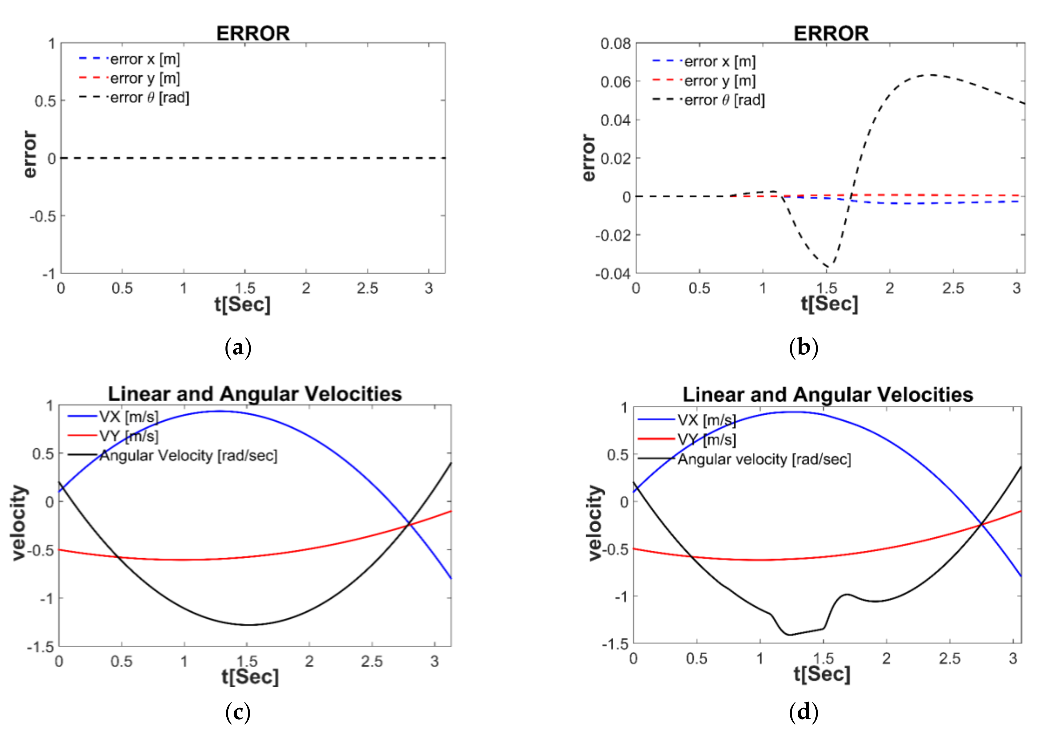
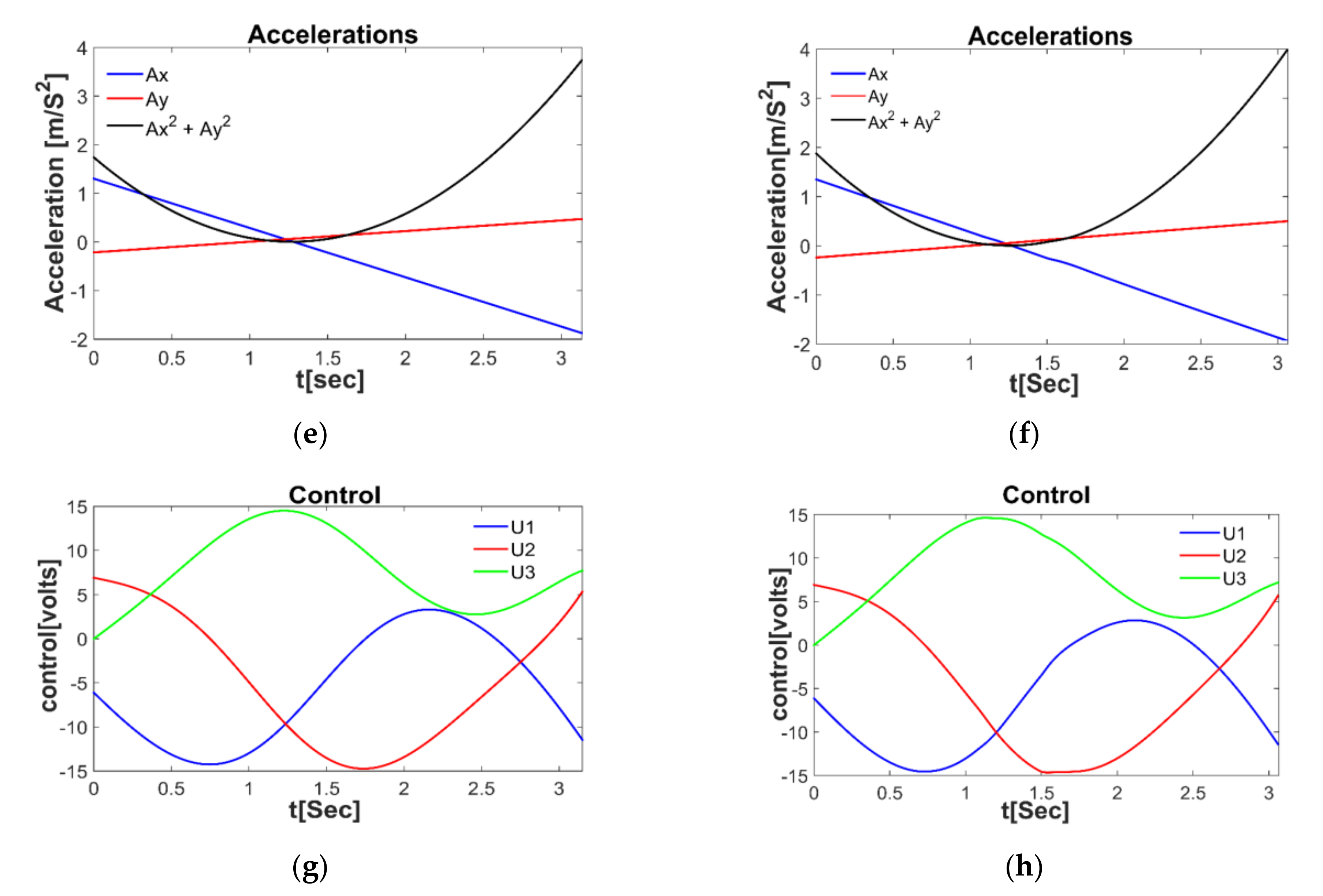
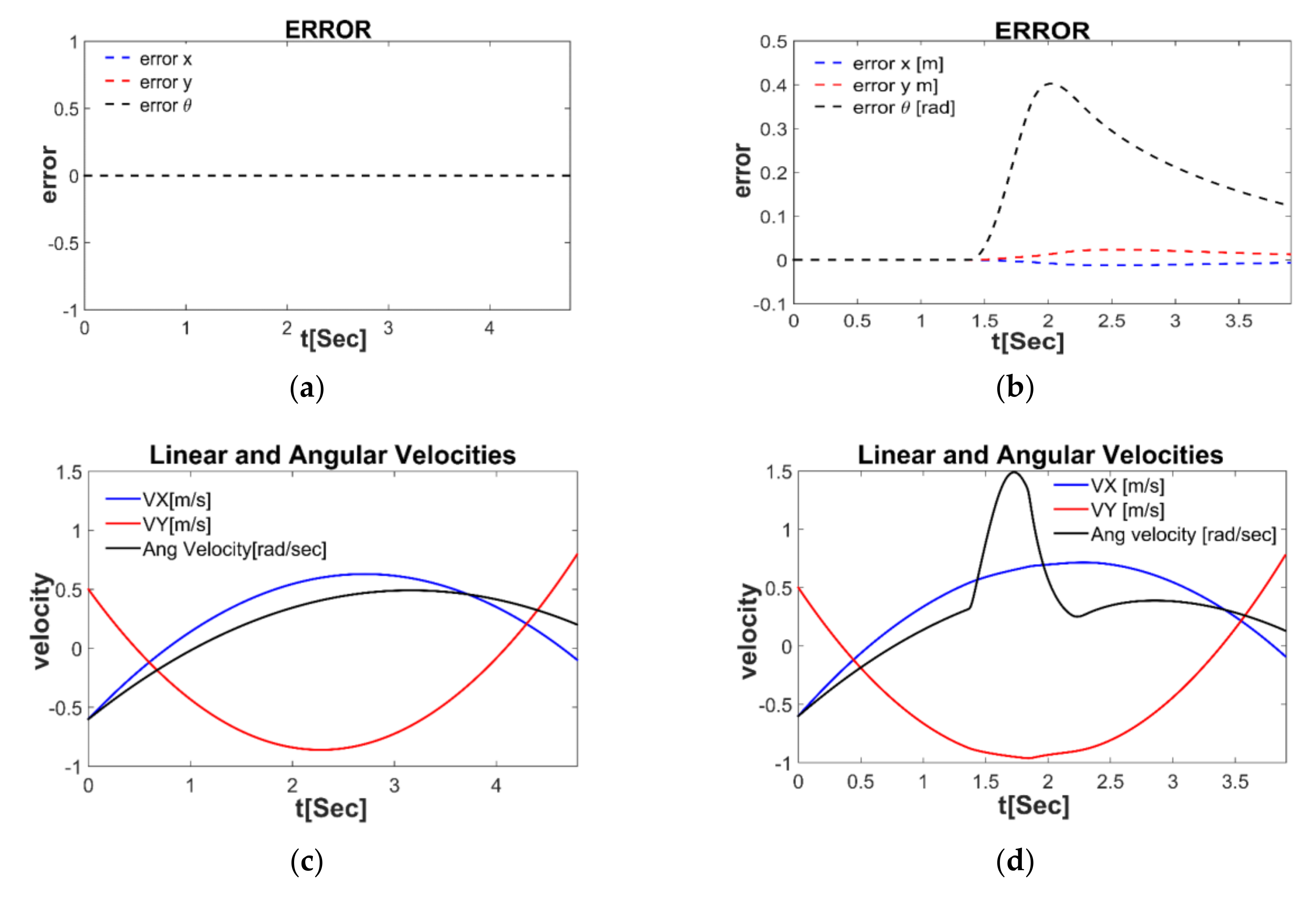
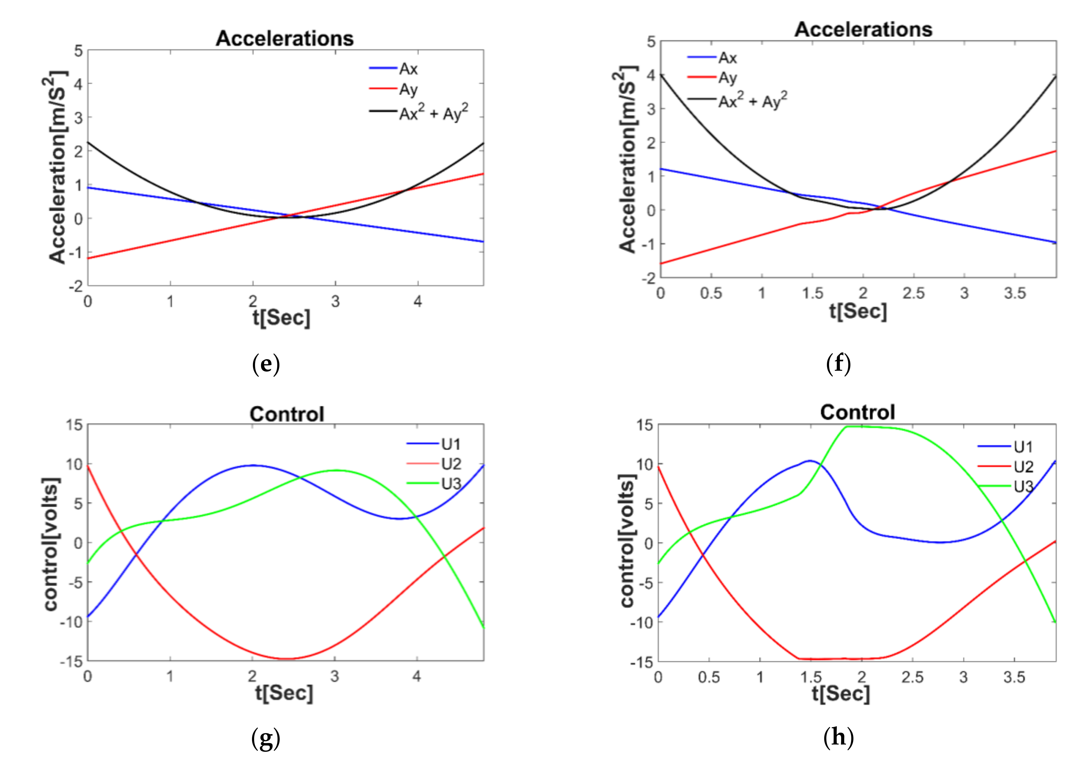
4. Validation and Experiment Process of the Representative Trajectories

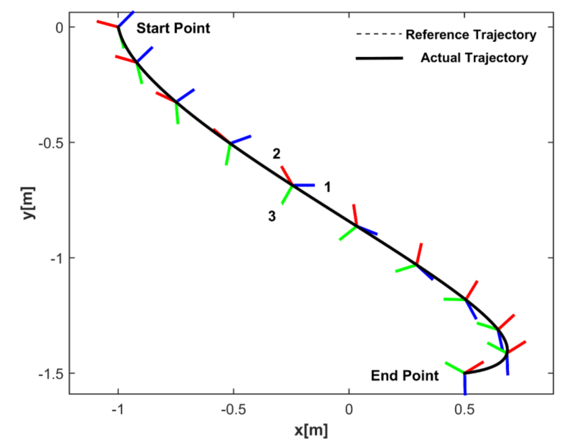
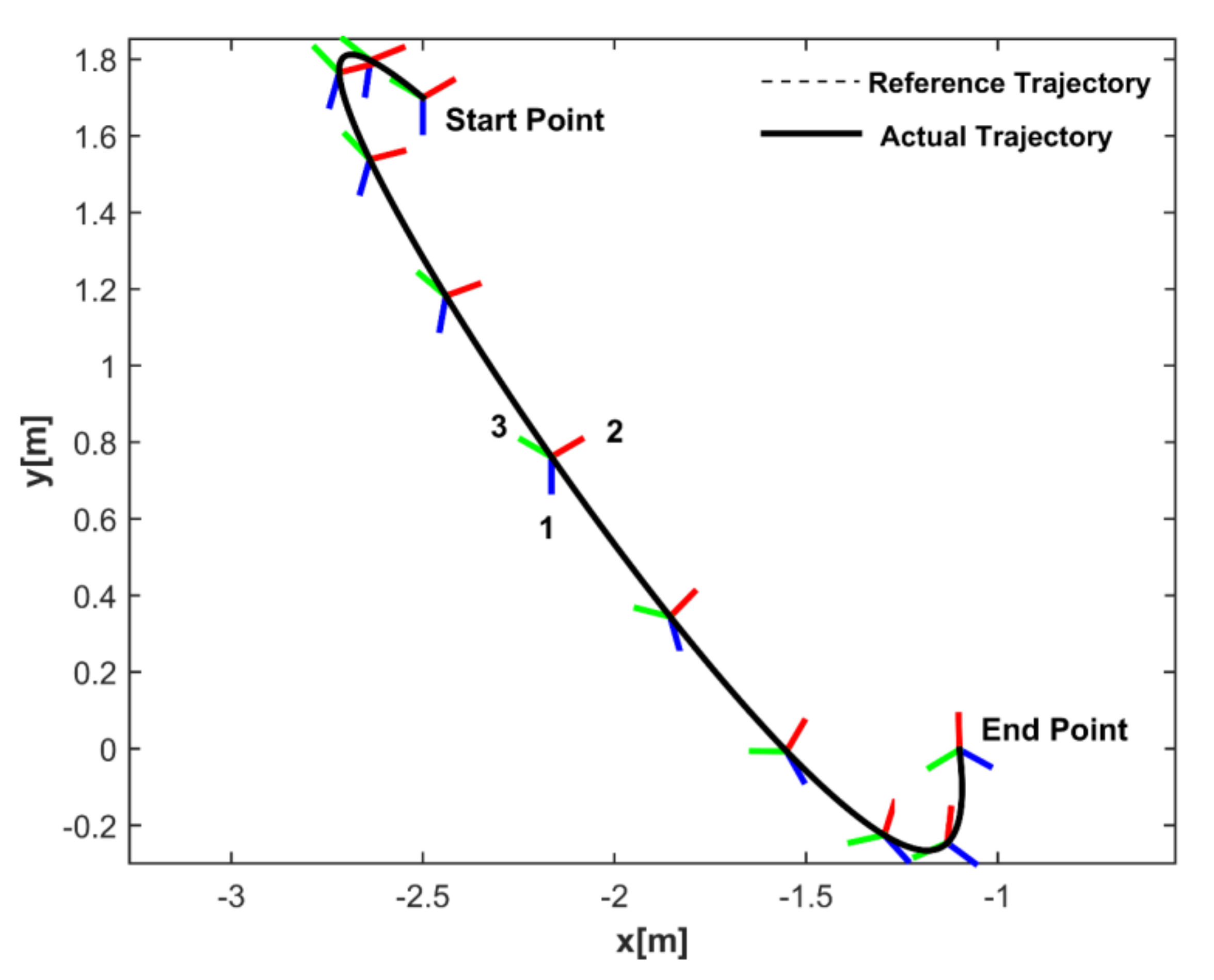
4.1. Simulation and Comparison Analysis

In this process, the method of solving the optimal control problem, Equation (25), proposed in the previous section was simulated, and a SAOWMR with three orthogonal wheels was be selected for utilization. In order to demonstrate the proposed method and show its effectiveness, the obtained simulation results are discussed and compared with those produced by the CDIB method presented in [53]. The CDIB method solves the optimal control problem by relaxing the terminal condition as an alternative to the direct handling of the constraint on the input voltage of the DC motors. Subsequently, it is only required that the actual final position and velocity at the end of the trajectory will be close enough to the initially planned ending position and velocity. Tracking error shown in Equation (59) is determined by constrained dynamic inversion-based (CDIB) method control law with saturation as follows:

$$e\left(t\right)=\mathrm{Z}\left(t\right)-{\mathrm{Z}}_{\mathrm{ref}}\left(t\right)$$

(59)

More details about the evolution of the tracking error while using the CDIB method can be found in [53]. The optimization problem to be solved by utilizing the CDIB method can be established by using the following fitness function:

$$\mathrm{Min} \mathrm{C}\left(t_{\mathrm{f}}\right)=t_{\mathrm{f}}+\zeta e_{\mathrm{terminl}} t_{\mathrm{f}}\in \left[\begin{array}{cc}{t}_{{\mathrm{f}}_{\min }}& t_{{\mathrm{f}}_{\max }}\end{array}\right]$$

(60)

In Equation (60), the lower bound $t_{{\mathrm{f}}_{\min }}$ is chosen so that the acceleration ${\ddot{x}}^2+{\ddot{y}}^2$ critically reaches the bound ${\alpha }_{\max }{}^2$ and can be found easily by using Equations (38) and (39). Moreover, $\zeta$ is a positive weight corresponding to the trade-off between the total maneuvering time $t_{\mathrm{f}}$ and the error concerning the intended and actual final position and velocity $e_{\mathrm{terminal}}$. The closeness of the CDIB method characterized by the terminal error $e_{\mathrm{terminal}}$ is expressed as follows:

$$e_{\mathrm{terminl}}={‖\mathrm{Z}\left(t=t_{\mathrm{f}}\right)-{\mathrm{Z}}_{\mathrm{ref}}\left(t=t_{\mathrm{f}}\right)‖}_2+{‖\dot{\mathrm{Z}}\left(t=t_{\mathrm{f}}\right)-{\dot{\mathrm{Z}}}_{\mathrm{ref}}\left(t=t_{\mathrm{f}}\right)‖}_2$$

(61)

To calculate the terminal error $e_{\mathrm{terminal}}$ stated in Equation (61), the actual trajectory should be calculated using the CDIB method so that the error along the trajectory will be stated. Then, $e_{\mathrm{terminal}}$ can be found. The required accuracies regarding the CDIB method are specified in

Table 1. Values used to produce the optimal trajectory of the robot using the CDIB method.

Parameter	Description	Value	Unit
$\left[\begin{array}{c}{e}_x\\ e_y\end{array}\right]$	Desired accuracy in distance	$\left[\begin{array}{c}0.02\\ 0.02\end{array}\right]$	m
$e_{\theta }$	Desired accuracy in orientation	0.12	rad
$\left[\begin{array}{c}{e}_{\dot{x}}\\ e_{\dot{y}}\end{array}\right]$	Desired accuracy in velocity	$\left[\begin{array}{c}0.02\\ 0.02\end{array}\right]$	m/s
$e_{\dot{\theta }}$	Desired accuracy in angular velocity	0.12	Rad/s
$\zeta$	Positive weight illustrating the trade-off between the maneuver time and the error	2

.

Solving the control problem illustrated in Equation (25) using the proposed method can be treated as a search for the final time $t_{\mathrm{f}}$ that minimizes the cost function C in Equation (36) so that a minimum bound $t_{{\mathrm{f}}_{\min }}$for the free variable $t_{\mathrm{f}}$ guarantees that the constraint system given in Equation (25) remains maintained. Finding an acceptable solution regarding the optimal final time $t_{\mathrm{f}}$ that minimizes the cost function C in Equation (36) involves implementing a simple golden-section search method since the energy is a monotonic function in terms of the free variable $t_{\mathrm{f}}$ varying within minimum and maximum bounds. Numerical values of the different parameters including robot and wheel motor characteristics used to produce the optimal trajectory regarding the two compared methods are illustrated in

Table 2. Values of the wheel motor characteristics used to demonstrate the trajectory.

Parameter	Description	Value	Unit
$k_{\tau }$	The torque constant of the robot	0.293	Nm/A
R	The armature resistance	1.465	Ω
$u_{\max }$	Limitation on the DC motor power source	14.8	V
$\alpha$	Characteristic constant	10	NV−1
$\beta$	Characteristic constant	146	Nsm−1

and

Table 3. Values of the robot characteristics used to demonstrate the trajectory.

Parameter	Description	Value	Unit
m	Mass of the vehicle	2.45	kg
J	Mass moment of inertia of the vehicle	0.00625	Kgm2
L	The radius of the SAOWMR	0.09	m
r	The radius of the robot wheels	0.02	m
${\alpha }_{\max }$	Limitations on the acceleration amplitude	2	ms−2

.

To find the global extreme solution $u_{\mathrm{o}i}$ of the input voltage function $u_i$ presented in Equation (32), the use of the simulated annealing algorithm is proposed.

Table 4. SA algorithm parameters.

Parameter	Value
Temperature reduction rule	Slow-decrease
Temperature update function	Exponential
Number of iterations per temperature	50
Maximum function evaluation	2500
Tolerance	10−3

presents the SA algorithm parameters selected to solve the optimization problem.

Moreover, the root-finding bisection method and the golden-section search method described in the proposed algorithm have a tolerance of ${10}^{-3}$. All the simulations, results, and graphs in this work were obtained using the MATLAB programing language. In order to determine the real-time performance, the proposed algorithm and the CDIB method were and compared in terms of the execution time using the C programing language. In order to evaluate and compare the results obtained by the proposed method with those produced by the CDIB method, two numerical tests were carried out. The boundary conditions of the testing maneuvers in SI units are given in

Table 5. Configurations of the two maneuvers.

Maneuvers	Starting Configurations	Termination Configurations
Maneuver 1	$\mathrm{Z}\left(0\right)=\left[\begin{array}{c}-1\\ 0\\ \pi /4\end{array}\right],\dot{\mathrm{Z}}\left(0\right)=\left[\begin{array}{c}0.1\\ -0.5\\ 0.2\end{array}\right]$	$\mathrm{Z}\left(t_{\mathrm{f}}\right)=\left[\begin{array}{c}0.5\\ -1.5\\ -\pi /2\end{array}\right],\dot{\mathrm{Z}}\left(t_{\mathrm{f}}\right)=\left[\begin{array}{c}-0.8\\ -0.1\\ 0.4\end{array}\right]$
Maneuver 2	$\mathrm{Z}\left(0\right)=\left[\begin{array}{c}-2.5\\ 1.7\\ -\pi /2\end{array}\right],\dot{\mathrm{Z}}\left(0\right)=\left[\begin{array}{c}-0.6\\ 0.5\\ -0.6\end{array}\right]$	$\mathrm{Z}\left(t_{\mathrm{f}}\right)=\left[\begin{array}{c}-1.1\\ 0\\ -\pi /6\end{array}\right],\dot{\mathrm{Z}}\left(t_{\mathrm{f}}\right)=\left[\begin{array}{c}-0.1\\ 0.8\\ 0.2\end{array}\right]$

.

Table 6. Trajectory optimization process result regarding maneuver 1 and maneuver 2.

Maneuvers	Method	Optimal Final Time	Terminal Error	Fitness Function	Code Execution Time (MATLAB)	Code Execution Time (C)
Maneuver 1	Proposed Method	3.1320 s	0.0000	3.1320	2.1265 s	0.06947 s
	CDIB [53]	3.0656 s	0.0044	3.0744	14.6981 s	1.68790 s
Maneuver 2	Proposed Method	4.7938 s	0.0000	4.7938	1.9827 s	0.06891 s
	CDIB [53]	3.9087 s	0.0206	3.9499	15.0198 s	1.49827 s

presents a comparison between the results obtained by utilizing the proposed method and those presented by the CDIB method regarding the best final time, termination error, and code execution time. As the method presented in [53] did not consider the total energy, the trade-off between the robot maneuvering time $t_{\mathrm{f}}$ and the total energy$\gamma$ in Equation (36) will be substituted by zero.

Both the proposed method and the CDIB method were implemented on a PC with Intel CORE i3 2.53 GHz CPU. However, the results show clearly that there is an intense improvement concerning the code execution time with an enhancement from around 1.68 s and 1.5 s in maneuvers 1 and 2, respectively, to almost 0.07 s. Moreover, it is clearly noticeable that the CDIB method attempts to minimize the terminal error produced by violating the constraint on the input voltage, but the proposed method attempts to converge to the exact optimal solution without producing any error. The optimal trajectories generated by the proposed method concerning maneuver 1 and maneuver 2 are given in the Figure 7 and Figure 8.

Figure 9 and Figure 10 demonstrate a comparison of the proposed method with the CDIB method presented in [53] in terms of the error evolution along the trajectory, the time histories of the linear and angular displacement of the center of mass of the robot, the acceleration of the center of mass along the trajectory, and the control inputs produced by both methods regarding maneuver 1 and maneuver 2.

The results shown in Figure 9 and Figure 10 illustrate how the proposed method successfully took into account the acceleration constraint and the constraint on the control inputs shown in Equation (25) concerning maneuver 1 and maneuver 2. The implementation of the golden-section search method to solve the optimization problem in Equation (36) was proposed since the energy E is a monotonic function in terms of the free variable $t_{\mathrm{f}}$ as shown in Figure 11. Figure 11 shows the evaluation of the energy E and the fitness function in Equation (36) with $\gamma =2$ evaluated at uniformly spaced points in the interval of the lower and upper bounds for the free variable $t_{\mathrm{f}}$ considering the two different maneuvers expressed in Table 5. Moreover, the optimal solutions obtained by utilizing the proposed method regarding maneuver 1 and maneuver 2 are clarified in Figure 11.

The results shown in Figure 11 illustrate clearly how the proposed method converges to the global minimum regarding the minimization problem given in Equation (36).

Table 7. Trajectory optimization process results regarding maneuver 1 and maneuver 2.

Maneuvers	Method	Trade-Off Value	${\mathit{t}}_{\mathbf{f}} \left(\mathbf{s}\right)$	E (J)
Maneuver 1	Proposed Method	$\gamma =0$	3.1320	3.7029
		$\gamma =2$	4.5103	2.4688
	CDIB [53]	-	3.0656	3.8327
Maneuver 2	Proposed Method	$\gamma =0$	4.7938	4.4805
		$\gamma =2$	5.7563	3.8798
	CDIB [53]	-	3.9087	5.4504

shows the effectiveness of utilizing the proposed method over the CDIB method in terms of total energy required to transport the robot regarding the two different maneuvers detailed in Table 5.

4.2. Study Discussion

In this study, the trajectory planning optimization problem of a SAOWMR with n omnidirectional wheels was defined as the process of estimating the control input vector U applied to the terminals of the DC motors attached to the robot’s wheels so that the robot can move from an initial configuration to a final configuration of boundary conditions with the optimality of the total maneuvering time $t_{\mathrm{f}}$ and the total required energy E while the constraint system remains maintained. The method proposed to solve the optimization problem is based on finding the optimal trajectory specified by selecting the total maneuvering time $t_{\mathrm{f}}$ over a set of an admissible range restricted by lower bound $t_{{\mathrm{f}}_{\min }}$ and upper bound $t_{{\mathrm{f}}_{\max }}$ so that the optimization problem is reduced to the one-dimensional search for the optimal total maneuvering time $t_{\mathrm{f}}$. A constraint system can arise due to various reasons. However, two essential constraints have been considered in this research: the constraint on the maximum acceleration amplitude and the constraint on the input voltage of the DC motors. The lower bound $t_{{\mathrm{f}}_{\min }}$regarding the free variable of the total maneuvering time $t_{\mathrm{f}}$ was proposed to be determined based on solving for the $t_{\mathrm{f}}$ so that the acceleration critically reaches the maximum bound and the maximum input voltage reaches the maximum limit. Consequently, the lower bound $t_{{\mathrm{f}}_{\min }}$ for the free variable $t_{\mathrm{f}}$ guarantees that the constraint system remains maintained. Moreover, the maximum bound $t_{{\mathrm{f}}_{\max }}$ of the free variable $t_{\mathrm{f}}$ can be selected based on the experience of the working environment and the specifications of the robot. Subsequently, a golden-section search method is implemented to ensure the optimality of the cost function constructed by the weight vector of the total maneuvering time $t_{\mathrm{f}}$ and the total required energy E.

The trajectory planning optimization proposed method was simulated and validated in order to demonstrate its effectiveness, utilizing a SAOWMR with three orthogonal wheels. The method was compared to another highly efficient trajectory planning optimization method called the constrained dynamic inversion-based (CDIB) method in order to show the effectiveness of our proposed method. The competing method, the CDIB method, solves the optimal control problem by relaxing the terminal conditions as an alternative to the direct handling of the constraint on the input voltage of the DC motors so that it is only required at the end of the trajectory, and the actual final position and velocity will be close enough to the initially planned ending position and velocity. The simulation process, including all the results and graphs obtained in this work, was conducted using MATLAB programing language. However, the proposed algorithm and the CDIB method were tested and compared in terms of the execution time using the C programing language. In order to perform a fair comparison, both the proposed method and the CDIB method were implemented on the same PC so that the error in the termination conditions and the code execution time of the two methods were taken into consideration. The results in Table 6 clearly present the effectiveness of the proposed method over the CDIB method in terms of the total execution time, showing that an intense enhancement was achieved. Moreover, the optimal trajectory produced by the proposed method converges to the exact optimal solution without producing any terminal error in contrast to the CDIB method that attempts to minimize the error in the terminal conditions. Another advantage of using the proposed method over the CDIB method with regard to the total energy required to transport the robot between two configurations is clarified in Table 7. Figure 11 clearly shows the convergence of the proposed method to the global optimal solution.

To sum up this discussion, several points highlight the novelty and the effectiveness of the proposed method over other methods in the field of trajectory planning optimization. First, the method proposed is based on the modeling of a SAOWMR with n omnidirectional wheels, making this method applicable for omnidirectional wheeled mobile robots that utilize three, four, five, or even more omnidirectional wheels. Second, the proposed method demonstrated real-time performance in which the optimal trajectory could be generated in less than 70 milliseconds. Moreover, the method proposed showed an accuracy performance of tending to generate the trajectory without any terminal error. Furthermore, while reaching the maximum limit of the input voltage of the wheel’s motor is sometimes undesirable, the proposed method enables the control of reaching the maximum limit by the factor $\gamma$ presented in Equation (25). Additionally, the incorporation of the path constraints such as obstacles with the proposed method of generating the optimal path is possible, as shown in Section 5.

5. Obstacle Avoidance

5.1. Problem Statement and Approach

The problem is stated as follows: a SAOWMR at a starting point must reach the ending point while avoiding collisions with static obstacles. In this section, a new computationally efficient obstacle avoidance motion planning method is proposed for a SAOWMR. The proposed method aims to incorporate the optimal control problem in Equation (25) with path constraints. The proposed obstacle avoidance method is summarized as follows: The well-known artificial potential field method will be utilized to generate a two-dimensional collision-free path between the starting and ending points. Hence, a particular number of equally arranged via points will be produced along the generated path. The attractive–repulsive potential parameters will be selected according to the actual dimensions of the robot and the workspace. Since the utilized path planning method addresses only x and y components, the robot orientation of the via points can be easily specified using the uniform distribution concept. Moreover, in order to determine appropriate velocity values of the via points, the cubic spline interpolation corresponding to the prospective value of the total maneuvering time will be utilized so that the third-order polynomial represents the trajectory between the adjacent points along the path. Based on the via points being distributed equally along the path, the total maneuvering time from the starting point to the ending point can be also be divided evenly into these portions of the overall trajectory. Subsequently, corresponding to the $j-1$ via points, the overall trajectory time $t_{{\mathrm{f}}_{\mathrm{T}}}$ will be portioned into j portions consisting of third-order polynomials as follows:

$$t_{{\mathrm{f}}_{\mathrm{T}}}={\displaystyle \sum _{\mathrm{c}=1}^j{t}_{{\mathrm{f}}_{\mathrm{c}}}}$$

(62)

The optimality of the trajectory can be specified by solving the minimization problem in the following equation:

$$\mathrm{Min} \mathrm{C}\left(t_{{\mathrm{f}}_{\mathrm{T}}}\right)=t_{{\mathrm{f}}_{\mathrm{T}}}+\gamma \mathrm{E} t_{{\mathrm{f}}_{\mathrm{T}}}\in \left[\begin{array}{cc}{t}_{{\mathrm{f}}_{{\mathrm{T}}_{\min }}}& t_{{\mathrm{f}}_{{\mathrm{T}}_{\max }}}\end{array}\right]$$

(63)

Equation (63) is solved by selecting the optimal total maneuvering time $t_{{\mathrm{f}}_{\mathrm{T}}}$ over a set of an admissible range restricted by lower bound and upper bound. The feasible domain of $t_{{\mathrm{f}}_{\mathrm{T}}}$ satisfies the constraint system of the input voltage and the acceleration discussed in Equation (25) in each portion of the overall trajectories. Moreover, $u_m$ is the maximum input voltage applied to the input terminals of the robot wheel DC motors along the overall trajectory calculated using the following formula:

$$u_m= \max \left\{u_{m1},u_{m2},\cdots ,u_{m j}\right\}$$

(64)

$u_{mi}$ is the maximum input voltage applied to the input terminals of the robot wheel DC motors along the portion i of the overall trajectory and can be found using Equation (26). The total maneuvering time $t_{{\mathrm{f}}_{\mathrm{T}}}{}_u$concerning the maximum input voltage $u_m$ reaching the maximum limit $u_{\max }$ can be determined by utilizing the simple root-finding bisection method. Furthermore, the total maneuvering time $t_{{\mathrm{f}}_{\mathrm{T}}}{}_{\mathrm{a}}$ concerning ${\ddot{x}}^2+{\ddot{y}}^2$ reaching the limit ${\alpha }_{\max }^2$ can also be determined by utilizing the simple root-finding bisection method. Consequently, the lower bound $t_{{\mathrm{f}}_{\mathrm{T}}}{}_{\min }$regarding the free variable $t_{{\mathrm{f}}_{\mathrm{T}}}$ can be obtained using the following relation:

$$t_{{\mathrm{f}}_{{\mathrm{T}}_{\min }}}= \max \left\{t_{{\mathrm{f}}_{{\mathrm{T}}_{\mathrm{u}}}},t_{{\mathrm{f}}_{{\mathrm{T}}_{\mathrm{a}}}}\right\}$$

(65)

With the above expansion, the optimal control problem in Equation (63) can be treated as a search for the final time $t_{{\mathrm{f}}_{\mathrm{T}}}$ that minimizes the cost function C. A minimum bound $t_{{\mathrm{f}}_{\mathrm{T}}}{}_{\min }$ for the free variable $t_{{\mathrm{f}}_{\mathrm{T}}}$ guarantees that the constraint system remains maintained. Maximum bound $t_{{\mathrm{f}}_{\mathrm{T}}}{}_{\max }$is chosen based on experience. In order to find an acceptable solution regarding the optimal final time $t_{{\mathrm{f}}_{\mathrm{T}}}$ that minimizes the cost function C in Equation (63), a simple golden-section search method can be easily implemented since the energy is a monotonic function in terms of the free variable $t_{{\mathrm{f}}_{\mathrm{T}}}$ varying within the minimum and maximum bounds.

5.2. Numerical Experiment and Simulations

The simulation described in this section demonstrates the real-time optimal obstacle avoidance trajectory generation proposed algorithm. The experiment involved the navigation of a SAOWMR with three orthogonal wheels from a starting configuration to a destination while avoiding some obstacles. The starting and destination configurations are stated in

Table 8. Starting and ending configurations regarding trajectories of the numerical tests.

Starting Point Configurations	Ending Point Configurations
$\mathrm{Z}\left(0\right)=\left[\begin{array}{c}9\\ 2\\ 0\end{array}\right],\dot{\mathrm{Z}}\left(0\right)=\left[\begin{array}{c}0\\ 0\\ 0\end{array}\right]$	$\mathrm{Z}\left(t_{\mathrm{f}}\right)=\left[\begin{array}{c}1\\ 8.5\\ \pi \end{array}\right],\dot{\mathrm{Z}}\left(t_{\mathrm{f}}\right)=\left[\begin{array}{c}0\\ 0\\ 0\end{array}\right]$

.

The system of obstacles used in this experiment consisted of four circular-shaped obstacles of 0.09 m radius separated in a 10 × 10 m field. The experimental results of using the artificial potential field method for the planning of the path between the starting point and the destination that ensures obstacle avoidance are shown in Figure 12.

In order to define appropriate velocity values of the via points, the cubic spline interpolation regarding the prospective value of the total maneuvering time was applied so that the third-order polynomial symbolizes the trajectory between the nearby via points along the generated path. The solution of the optimal control problem and the generation of the real-time collision-free optimal trajectory using the proposed method are demonstrated clearly in Figure 13 and Figure 14.

Figure 13 shows how the SAOWMR with three orthogonal wheels successfully navigates from the initial configuration to the destination point, passing through all the via points while sufficiently avoiding all the obstacles. Moreover, Figure 14 illustrates the control input voltage of the robot wheels that must be tracked and used by the robot controller. The proposed method clearly shows the satisfaction of dynamic and path constraints, as well as the smoothness of the motion control. Furthermore, the proposed obstacle avoidance method achieved a good result regarding the execution time with less than 100 milliseconds for generating the optimal trajectory, placing this method within the computationally effective algorithms.

6. Conclusions

This paper presents a compact and complete mathematical model for a symmetrical annular-shaped omnidirectional wheeled mobile robot (SAOWMR). This model provides an opportunity to derive the equations of motion of a SAOWMR with $n$ omnidirectional wheels effortlessly without the necessity to switch models or derive a new model. The paper proposes a new computationally effective method for achieving improvements in trajectory planning optimization (TPO) for a SAOWMR with $n$ omnidirectional wheels. The experiments show that the optimal trajectory generated by the proposed method effectively satisfies the constraint system and demonstrates remarkable improvements in terms of accuracy and low complexity. The method proposed has been tested in collision-free navigation by the incorporation of the path constraints.

Future work will focus on completing the research by testing and optimizing a real prototype utilizing vision-based system to achieve navigation processes such as ball catching and obstacle avoidance in dynamic environments.

References

1. Mariappan, M.; Sing, J.C.; Wee, C.C.; Khoo, B.; Wong, W.K. Simultaneous Rotation and Translation Movement for Four Omnidirectional Wheels Holonomic Mobile Robot. In Proceedings of the 2014 IEEE International Symposium on Robotics and Manufacturing Automation (ROMA), Kuala Lumpur, Malaysia, 15–16 December 2014; pp. 69–73. [Google Scholar]
2. Kale, S.; Shriramwar, S.S. FPGA-Based Controller for a Mobile Robot. arXiv 2009, arXiv:0908.221. [Google Scholar]
3. Endo, G.; Hirose, S. Study on roller-walker (system integration and basic experiments). In Proceedings of the 1999 IEEE International Conference on Robotics and Automation (Cat. No.99CH36288C), Detroit, MI, USA, 10–15 May 1999; Volume 3, pp. 2032–2037. [Google Scholar]
4. Yu, H.; Spenko, M.; Dubowsky, S. Omni-Directional Mobility Using Active Split Offset Castors. J. Mech. Des. 2004, 126, 822–829. [Google Scholar] [CrossRef]
5. Grabowiecki, J. Vehicle Wheel. U.S. Patent No. 1,303,535, 3 June 1919. [Google Scholar]
6. Ilon, B.E. Wheels for a Course Stable Selfpropelling Vehicle Movable in Any Desired Direction on the Ground or Some Other Base. U.S. Patent No. 3,876,255, 8 April 1975. [Google Scholar]
7. Podnar, G.W. The Uranus Mobile Robot. In Autonomous Mobile Robots: Annual Report; Carnagie Melon University: Pittsburgh, PA, USA, 1985. [Google Scholar]
8. Muir, P.F.; Neuman, C.P. Kinematic Modeling of Wheeled Mobile Robots. J. Robot. Syst. 1987, 4, 281–340. [Google Scholar] [CrossRef]
9. Koestler, A.; Braunl, T. Mobile Robot Simulation with Realistic Error Models. In Proceedings of the Second International Conference on Autonomous Robots and Agents, Massey University, Palmerston North, New Zealand, 13–15 December 2004; pp. 46–51. [Google Scholar]
10. Song, J.-B.; Byun, K.-S. Design and Control of a Four-Wheeled Omnidirectional Mobile Robot with Steerable Omnidirectional Wheels. J. Robot. Syst. 2004, 21, 193–208. [Google Scholar] [CrossRef]
11. Salih, J.E.M.; Rizon, M.; Yaacob, S.; Adom, A.H.; Mamat, M.R. Designing Omni-Directional Mobile Robot with Mecanum Wheel. Am. J. Appl. Sci. 2006, 3, 1831–1835. [Google Scholar] [CrossRef]
12. Qian, J.; Zi, B.; Wang, D.; Ma, Y.; Zhang, D. The Design and Development of an Omni-Directional Mobile Robot Oriented to an Intelligent Manufacturing System. Sensors 2017, 17, 2073. [Google Scholar] [CrossRef] [Green Version]
13. Doroftei, I.; Grosu, V.; Spinu, V. Omnidirectional Mobile Robot-Design and Implementation; IntechOpen: London, UK, 2007; ISBN 978-3-902613-15-8. [Google Scholar]
14. Dickerson, S.L.; Lapin, B.D. Control of an Omni-Directional Robotic Vehicle with Mecanum Wheels. In Proceedings of the NTC ’91-National Telesystems Conference Proceedings, Atlanta, GA, USA, 26–27 March 1991; pp. 323–328. [Google Scholar]
15. Nagatani, K.; Tachibana, S.; Sofue, M.; Tanaka, Y. Improvement of Odometry for Omnidirectional Vehicle Using Optical Flow Information. In Proceedings of the 2000 IEEE/RSJ International Conference on Intelligent Robots and Systems, Takamatsu, Japan, 31 October–5 November 2000. [Google Scholar]
16. Pin, F.G.; Killough, S.M. A New Family of Omnidirectional and Holonomic Wheeled Platforms for Mobile Robots. IEEE Trans. Robot. Autom. 1994, 10, 480–489. [Google Scholar] [CrossRef]
17. Byun, K.-S.; Song, J.-B. Design and Construction of Continuous Alternate Wheels for an Omnidirectional Mobile Robot. J. Robot. Syst. 2003, 20, 569–579. [Google Scholar] [CrossRef]
18. West, M.; Asada, H. Design and Control of Ball Wheel Omnidirectional Vehicles. In Proceedings of the 1995 IEEE International Conference on Robotics and Automation, Nagoya, Japan, 21–27 May 1995; Volume 2, pp. 1931–1938. [Google Scholar]
19. Li, Y.; Dai, S.; Zhao, L.; Yan, X.; Shi, Y. Topological Design Methods for Mecanum Wheel Configurations of an Omnidirectional Mobile Robot. Symmetry 2019, 11, 1268. [Google Scholar] [CrossRef] [Green Version]
20. Gfrerrer, A. Geometry and Kinematics of the Mecanum Wheel. Comput. Aided Geom. Des. 2008, 25, 784–791. [Google Scholar] [CrossRef]
21. Gao, P.; Peng, J.; Yu, W.; Li, S.; Qin, X. Design and Motion Analysis of a Mecanum Three-Round Omni-Directional Mobile Platform. J. Northwestern Polytech. Univ. 2017, 35, 857–862. [Google Scholar]
22. Lafaye, J.; Gouaillier, D.; Wieber, P.-B. Linear Model Predictive Control of the Locomotion of Pepper, a Humanoid Robot with Omnidirectional Wheels. In Proceedings of the 2014 IEEE-RAS International Conference on Humanoid Robots, Madrid, Spain, 18–20 November 2014; pp. 336–341. [Google Scholar]
23. Song, J.B.; Byun, K.S. Steering Control Algorithm for Efficient Drive of a Mobile Robot with Steerable Omni-Directional Wheels. J. Mech. Sci. Technol. 2009, 23, 2747–2756. [Google Scholar] [CrossRef]
24. Tian, Y.; Zhang, S.; Liu, J.; Chen, F.; Li, L.; Xia, B. Research on a New Omnidirectional Mobile Platform with Heavy Loading and Flexible Motion. Adv. Mech. Eng. 2017, 9. [Google Scholar] [CrossRef]
25. Muir, P.F.; Neuman, C.P. Kinematic Modeling for Feedback Control of an Omnidirectional Wheeled Mobile Robot. In Autonomous Robot Vehicles; Springer: New York, NY, USA, 1990; pp. 25–31. [Google Scholar]
26. Wieczorek, B. Methods of Determining Trajectory for Wheelchair with Manual Pushrims Drive. IOP Conf. Ser. Mater. Sci. Eng. 2021, 1016, 012004. [Google Scholar] [CrossRef]
27. Wieczorek, B.; Kukla, M. Biomechanical Relationships Between Manual Wheelchair Steering and the Position of the Human Body’s Center of Gravity. J. Biomech. Eng. 2020, 142. [Google Scholar] [CrossRef]
28. Leow, Y.P.; Low, K.H.; Loh, W.K. Kinematic Modelling and Analysis of Mobile Robots with Omni-Directional Wheels. In Proceedings of the 7th International Conference on Control, Automation, Robotics and Vision, Singapore, 2–5 December 2002; Volume 2, pp. 820–825. [Google Scholar]
29. Loh, W.K.; Low, K.H.; Leow, Y.P. Mechatronics Design and Kinematic Modelling of a Singularityless Omni-Directional Wheeled Mobile Robot. In Proceedings of the 2003 IEEE International Conference on Robotics and Automation (Cat. No.03CH37422), Taipei, Taiwan, 14–19 September 2003; Volume 3, pp. 3237–3242. [Google Scholar]
30. Watanabe, K. Control of an Omnidirectional Mobile Robot. In Proceedings of the 1998 Second International Conference, Knowledge-Based Intelligent Electronic Systems, Adelaide, South Australia, 21–23 April 1998; Volume 1, pp. 51–60. [Google Scholar]
31. Li, X.; Zell, A. Motion Control of an Omnidirectional Mobile Robot. In Informatics in Control, Automation and Robotics: Selected Papers from the International Conference on Informatics in Control, Automation and Robotics; Springer: Berlin/Heidelberg, Germany, 2009; pp. 181–193. ISBN 978-3-540-85640-5. [Google Scholar]
32. Kalmár-Nagy, T.; D’Andrea, R.; Ganguly, P. Near-Optimal Dynamic Trajectory Generation and Control of an Omnidirectional Vehicle. Robot. Auton. Syst. 2004, 46, 47–64. [Google Scholar] [CrossRef]
33. Purwin, O.; D’Andrea, R. Trajectory Generation and Control for Four Wheeled Omnidirectional Vehicles. Robot. Auton. Syst. 2006, 54, 13–22. [Google Scholar] [CrossRef]
34. Kalmar-Nagy, T.; Ganguly, P.; D’Andrea, R. Real-Time Trajectory Generation for Omnidirectional Vehicles. In Proceedings of the 2002 American Control Conference (IEEE Cat. No.CH37301), Anchorage, AK, USA, 8–10 May 2002; Volume 1, pp. 286–291. [Google Scholar]
35. Alwan, H.M. Dynamic Analysis Modeling of a Holonomic Wheeled Mobile Robot with Mecanum Wheels Using Virtual Work Method. J. Mech. Eng. Res. Dev. 2020, 43, 373–380. [Google Scholar]
36. Hou, L.; Zhang, L.; Kim, J. Energy Modeling and Power Measurement for Mobile Robots. Energies 2019, 12, 27. [Google Scholar] [CrossRef] [Green Version]
37. Alwan, H.M.; Volkov, A.N.; Shbani, A. Solution of Inverse and Forward Kinematics Problems for Mobile Robot with Six Mecanum Wheels. IOP Conf. Ser. Mater. Sci. Eng. 2021, 1094, 012071. [Google Scholar] [CrossRef]
38. Rijalusalam, D.U.; Iswanto, I. Implementation Kinematics Modeling and Odometry of Four Omni Wheel Mobile Robot on The Trajectory Planning and Motion Control Based Microcontroller. J. Robot. Control 2021, 2, 448–455. [Google Scholar] [CrossRef]
39. Karras, G.C.; Fourlas, G.K. Model Predictive Fault Tolerant Control for Omni-Directional Mobile Robots. J. Intell. Robot. Syst. 2020, 97, 635–655. [Google Scholar] [CrossRef]
40. Cuevas, F.; Castillo, O.; Cortés-Antonio, P. Omnidirectional Four Wheel Mobile Robot Control with a Type-2 Fuzzy Logic Behavior-Based Strategy. In Intuitionistic and Type-2 Fuzzy Logic Enhancements in Neural and Optimization Algorithms: Theory and Applications; Studies in Computational Intelligence; Springer International Publishing: Cham, Switzerland, 2020; pp. 49–62. ISBN 978-3-030-35445-9. [Google Scholar]
41. Yang, H.; Wang, S.; Zuo, Z.; Li, P. Trajectory Tracking for a Wheeled Mobile Robot with an Omnidirectional Wheel on Uneven Ground. IET Control Theory Appl. 2020, 14, 921–929. [Google Scholar] [CrossRef]
42. Serrano-Pérez, O.; Villarreal-Cervantes, M.G.; González-Robles, J.C.; Rodríguez-Molina, A. Meta-Heuristic Algorithms for the Control Tuning of Omnidirectional Mobile Robots. Eng. Optim. 2020, 52, 325–342. [Google Scholar] [CrossRef]
43. Abiyev, R.H.; Günsel, I.S.; Akkaya, N.; Aytac, E.; Çağman, A.; Abizada, S. Fuzzy Control of Omnidirectional Robot. Procedia Comput. Sci. 2017, 120, 608–616. [Google Scholar] [CrossRef]
44. Abiyev, R.H.; Akkaya, N.; Gunsel, I. Control of Omnidirectional Robot Using Z-Number-Based Fuzzy System. IEEE Trans. Syst. Man Cybern. Syst. 2019, 49, 238–252. [Google Scholar] [CrossRef]
45. Hacene, N.; Mendil, B. Motion Analysis and Control of Three-Wheeled Omnidirectional Mobile Robot. J. Control. Autom. Electr. Syst. 2019, 30, 194–213. [Google Scholar] [CrossRef]
46. Alshorman, A.M.; Alshorman, O.; Irfan, M.; Glowacz, A.; Muhammad, F.; Caesarendra, W. Fuzzy-Based Fault-Tolerant Control for Omnidirectional Mobile Robot. Machines 2020, 8, 55. [Google Scholar] [CrossRef]
47. Wang, C.; Liu, X.; Yang, X.; Hu, F.; Jiang, A.; Yang, C. Trajectory Tracking of an Omni-Directional Wheeled Mobile Robot Using a Model Predictive Control Strategy. Appl. Sci. 2018, 8, 231. [Google Scholar] [CrossRef] [Green Version]
48. Thi, K.D.H.; Nguyen, M.C.; Vo, H.T.; Tran, V.M.; Nguyen, D.D.; Bui, A.D. Trajectory Tracking Control for Four-Wheeled Omnidirectional Mobile Robot Using Backstepping Technique Aggregated with Sliding Mode Control. In Proceedings of the 2019 First International Symposium on Instrumentation, Control, Artificial Intelligence, and Robotics (ICA-SYMP), Bangkok, Thailand, 16–18 January 2019; pp. 131–134. [Google Scholar]
49. Xie, Y.; Zhang, X.; Meng, W.; Xie, S.; Jiang, L.; Meng, J.; Wang, S. Coupled Sliding Mode Control of an Omnidirectional Mobile Robot with Variable Modes. In Proceedings of the 2020 IEEE/ASME International Conference on Advanced Intelligent Mechatronics (AIM), Boston, MA, USA, 6–9 July 2020; pp. 1792–1797. [Google Scholar]
50. Dong, F.; Jin, D.; Zhao, X.; Han, J. Adaptive Robust Constraint Following Control for Omnidirectional Mobile Robot: An Indirect Approach. IEEE Access 2021, 9, 8877–8887. [Google Scholar] [CrossRef]
51. Sahoo, S.R.; Chiddarwar, S.S. Flatness-Based Control Scheme for Hardware-in-the-Loop Simulations of Omnidirectional Mobile Robot. SIMULATION 2020, 96, 169–183. [Google Scholar] [CrossRef]
52. Amudhan, A.N.; Sakthivel, P.; Sudheer, A.P.; Kumar, T.K.S. Design of Controllers for Omnidirectional Robot Based on the Ystem Identification Technique for Trajectory Tracking. J. Phys. Conf. Ser. 2019, 1240, 012146. [Google Scholar] [CrossRef]
53. Kalmár-Nagy, T. Real-Time Trajectory Generation for Omni-Directional Vehicles by Constrained Dynamic Inversion. Mechatronics 2016, 35, 44–53. [Google Scholar] [CrossRef]
54. Wu, M.; Dai, S.-L.; Yang, C. Mixed Reality Enhanced User Interactive Path Planning for Omnidirectional Mobile Robot. Appl. Sci. 2020, 10, 1135. [Google Scholar] [CrossRef] [Green Version]
55. Saenz, A.; Santibañez, V.; Bugarin, E.; Dzul, A.; Ríos, H.; Villalobos-Chin, J. Velocity Control of an Omnidirectional Wheeled Mobile Robot Using Computed Voltage Control with Visual Feedback: Experimental Results. Int. J. Control. Autom. Syst. 2021, 19, 1089–1102. [Google Scholar] [CrossRef]
56. Ou, J.; Wang, M. Path Planning for Omnidirectional Wheeled Mobile Robot by Improved Ant Colony Optimization. In Proceedings of the 2019 Chinese Control Conference (CCC), Guangzhou, China, 27–30 July 2019; pp. 2668–2673. [Google Scholar]
57. Choi, J.; Curry, R.E.; Elkaim, G.H. Obstacle Avoiding Real-Time Trajectory Generation and Control of Omnidirectional Vehicles. In Proceedings of the 2009 American Control Conference, St. Louis, MO, USA, 10–12 June 2009; pp. 5510–5515. [Google Scholar]
58. Azim Mohseni, N.; Fakharian, A. Direct Optimal Motion Planning for Omni-Directional Mobile Robots under Limitation on Velocity and Acceleration. J. Optim. Ind. Eng. 2017, 10, 93–101. [Google Scholar] [CrossRef]
59. Williams, R.L.; Wu, J. Dynamic Obstacle Avoidance for an Omnidirectional Mobile Robot. J. Robot. 2010, 2010. [Google Scholar] [CrossRef] [Green Version]
60. Liu, X.; Chen, H.; Wang, C.; Hu, F.; Yang, X. MPC Control and Path Planning of Omni-Directional Mobile Robot with Potential Field Method. In Proceedings of the Intelligent Robotics and Applications, Newcastle, NSW, Australia, 9–11 August 2018; Springer International Publishing: Cham, Switzerland, 2018; pp. 170–181. [Google Scholar]
61. Guo, S.; Diao, Q.; Xi, F. Vision Based Navigation for Omni-Directional Mobile Industrial Robot. Procedia Comput. Sci. 2017, 105, 20–26. [Google Scholar] [CrossRef]
62. Kim, C.; Suh, J.; Han, J.-H. Development of a Hybrid Path Planning Algorithm and a Bio-Inspired Control for an Omni-Wheel Mobile Robot. Sensors 2020, 20, 4258. [Google Scholar] [CrossRef]
63. Azizi, M.R.; Rastegarpanah, A.; Stolkin, R. Motion Planning and Control of an Omnidirectional Mobile Robot in Dynamic Environments. Robotics 2021, 10, 48. [Google Scholar] [CrossRef]
64. Cuevas, F.; Castillo, O.; Cortes-Antonio, P. Towards an Adaptive Control Strategy Based on Type-2 Fuzzy Logic for Autonomous Mobile Robots. In Proceedings of the 2019 IEEE International Conference on Fuzzy Systems (FUZZ-IEEE), New Orleans, LA, USA, 23–26 June 2019; pp. 1–6. [Google Scholar]
65. Hacene, N.; Mendil, B. Fuzzy Behavior-Based Control of Three Wheeled Omnidirectional Mobile Robot. Int. J. Autom. Comput. 2019, 16, 163–185. [Google Scholar] [CrossRef]
66. Ajeil, F.H.; Ibraheem, I.K.; Azar, A.T.; Humaidi, A.J. Autonomous Navigation and Obstacle Avoidance of an Omnidirectional Mobile Robot Using Swarm Optimization and Sensors Deployment. Int. J. Adv. Robot. Syst. 2020, 17. [Google Scholar] [CrossRef]
67. Thakur, N.; Han, C.Y. Multimodal Approaches for Indoor Localization for Ambient Assisted Living in Smart Homes. Information 2021, 12, 114. [Google Scholar] [CrossRef]
68. Zhang, Y.; Zhang, C.-H.; Shao, X. User Preference-Aware Navigation for Mobile Robot in Domestic via Defined Virtual Area. J. Netw. Comput. Appl. 2021, 173, 102885. [Google Scholar] [CrossRef]
69. Ran, T.; Yuan, L.; Zhang, J.B. Scene Perception Based Visual Navigation of Mobile Robot in Indoor Environment. ISA Trans. 2021, 109, 389–400. [Google Scholar] [CrossRef]
70. Gamal, O.; Cai, X.; Roth, H. Learning from Fuzzy System Demonstration: Autonomous Navigation of Mobile Robot in Static Indoor Environment Using Multimodal Deep Learning. In Proceedings of the 2020 24th International Conference on System Theory, Control and Computing (ICSTCC), Sinaia, Romania, 8–10 October 2020; pp. 218–225. [Google Scholar]
71. Al Khatib, E.I.; Jaradat, M.A.K.; Abdel-Hafez, M.F. Low-Cost Reduced Navigation System for Mobile Robot in Indoor/Outdoor Environments. IEEE Access 2020, 8, 25014–25026. [Google Scholar] [CrossRef]
72. Iqbal, J.; Xu, R.; Sun, S.; Li, C. Simulation of an Autonomous Mobile Robot for LiDAR-Based In-Field Phenotyping and Navigation. Robotics 2020, 9, 46. [Google Scholar] [CrossRef]
73. Bai, X.; Dong, L.; Ge, L.; Xu, H.; Zhang, J.; Yan, J. Robust Localization of Mobile Robot in Industrial Environments With Non-Line-of-Sight Situation. IEEE Access 2020, 8, 22537–22545. [Google Scholar] [CrossRef]
74. Kim, E.-K.; Kim, S.-S. Generation of Feature Map for Improving Localization of Mobile Robot Based on Stereo Camera. J. Korea Inst. Inf. Electron. Commun. Technol. 2020, 13, 58–63. [Google Scholar] [CrossRef]
75. Li, H.; Mao, Y.; You, W.; Ye, B.; Zhou, X. A Neural Network Approach to Indoor Mobile Robot Localization. In Proceedings of the 2020 19th International Symposium on Distributed Computing and Applications for Business Engineering and Science (DCABES), Xuzhou, China, 16–19 October 2020; pp. 66–69. [Google Scholar]
76. Greenberg, J.N.; Tan, X. Dynamic Optical Localization of a Mobile Robot Using Kalman Filtering-Based Position Prediction. IEEE/ASME Trans. Mechatron. 2020, 25, 2483–2492. [Google Scholar] [CrossRef]
Figure 1. Types of the omnidirectional wheels and their trails: (a) the primitive design of the orthogonal wheels contains multiple inner rollers surrounding the wheel structure where the axes of these rollers are orthogonal to the axis of the wheel; (b) an omnidirectional wheel where its passive rollers are mounted on angles in an attempt to achieve continuous contact between the wheel and the ground, called the Mecanum wheel; (c) a wheel based on the dual overlapping orthogonal wheel, patented as a modified version of the conventional orthogonal wheel; (d) an enhanced version of the orthogonal wheel designed based on the use of inner and outer passive rollers to ensure continuous contact between the wheel and the ground; (e) the ball wheel mechanism, which is based on the use of two arrays of rollers disposed around two circles and an active ring capable of rotating around an axis through the center of the ball.
Symmetry 13 01033 g001
Figure 2. The configurations of the omnidirectional wheel.
Symmetry 13 01033 g002
Figure 3. The configuration of a SAOWMR with n wheels.
Symmetry 13 01033 g003
Figure 4. The topological designs of SAOWMRs: (af) the structures of SAOWMRs with two, three, four, five, six, and eight omnidirectional orthogonal wheels, respectively.
Symmetry 13 01033 g004
Figure 5. Real prototype of a SAOWMR with 3 omnidirectional wheels.
Symmetry 13 01033 g005
Figure 6. The geometry of the SAOWMR.
Symmetry 13 01033 g006
Figure 7. Optimal trajectory generated by the proposed method regarding maneuver 1.
Symmetry 13 01033 g007
Figure 8. Optimal trajectory generated by the proposed method regarding maneuver 2.
Symmetry 13 01033 g008
Figure 9. Comparison of the proposed method with the CDIB method regarding maneuver 1: (a,c,e,g) the error evolution along the trajectory, the time histories of the linear and angular displacement, the acceleration along the trajectory, and the control inputs generated by the proposed method, respectively; (b,d,f,h) the error evolution along the trajectory, the time histories of the linear and angular displacement, the acceleration along the trajectory, and the control inputs generated by the CDIB method, respectively.
Symmetry 13 01033 g009aSymmetry 13 01033 g009b
Figure 10. Comparison of the proposed method with the CDIB method regarding maneuver 2: (a,c,e,g) the error evolution along the trajectory, the time histories of the linear and angular displacement, the acceleration along the trajectory, and the control inputs generated by the proposed method, respectively; (b,d,f,h) the error evolution along the trajectory, the time histories of the linear and angular displacement, the acceleration along the trajectory, and the control inputs generated by the CDIB method, respectively.
Symmetry 13 01033 g010aSymmetry 13 01033 g010b
Figure 11. Energy and fitness function evaluation and demonstration of the optimal solutions regarding two different maneuvers: (a,b) the energy evaluation at uniformly spaced points for the free variable t f regarding maneuver 1 and maneuver 2, respectively; (c,d) the fitness function in Equation (36) with γ = 2 evaluated at uniformly spaced points in order to demonstrate the convergence to the optimal solutions regarding maneuver 1 and maneuver 2, respectively.
Symmetry 13 01033 g011aSymmetry 13 01033 g011b
Figure 12. Path planning using artificial potential field method.
Symmetry 13 01033 g012
Figure 13. Real-time collision-free optimal trajectory generated between starting and ending points using the proposed obstacle avoidance method.
Symmetry 13 01033 g013
Figure 14. Control input voltages of the robot wheels produced by the proposed algorithm to be used by the robot controller.
Symmetry 13 01033 g014