An Extension TOPSIS Method Based on the Decision Maker’s Risk Attitude and the Adjusted Probabilistic Fuzzy Set

Abstract

The paper studies an extension TOPSIS method with the adjusted probabilistic linguistic fuzzy set in which the decision maker’s behavior tendency is considered. Firstly, we propose a concept of probabilistic linguistic q-rung orthopair set (PLQROS) based on the probability linguistic fuzzy set (PLFS) and linguistic q-rung orthopair set (LQROS). The operational laws are introduced based on the transformed probabilistic linguistic q-rung orthopair sets (PLQROSs) which have the same probability. Through this adjustment method, the irrationality of the existing methods in the aggregation process is avoided. Furthermore, we propose a comparison rule of PLQROS and the aggregated operators. The distance measure of PLQROSs is also defined, which can deal with the symmetric information in multi-attribute decision making problems. Considering that the decision maker’s behavior has a very important impact on decision-making results, we propose a behavioral TOPSIS decision making method for PLQROS. Finally, we apply the practical problem of investment decision to demonstrate the validity of the extension TOPSIS method, and the merits of the behavior decision method is testified by comparing with the classic TOPSIS method. The sensitivity analysis results of decision-maker’s behavior are also given.

1. Introduction

There is much uncertainty in decision making problems. It is not easy to describe the evaluation information with accurate numerical value, and they can only be described with linguistic values. Zadeh [1,2,3] defined the linguistic term set (LTS) and applied it to express the qualitative evaluation. For example, the commonly used seven valued LTS is in the form of $S=\{s_0:greatdistaste,s_1:distaste,s_2:abitdistaste,s_3:generally,s_4:abitfavorite,s_5:favorite,s_6:greatfavorite\}$, it can be used to describe how much the decision maker likes the object. However, when the decision maker hesitates about the preference of the evaluation object, the single linguistic term is no longer describe such information. So Rodríguez et al. [4] presented the hesitant fuzzy linguistic term set (HFLTS), each of elements is a collection of linguistic terms. For example, the decision maker thinks that the audience’s opinion of the program is “favorite” or “great favorite”, the evaluation about the opinion of the program can be only expressed in the form of $\{s_5,s_6\}$. Since the HFLTS was put forward, some extensions of HFLTS were developed and applied in many fields [5,6,7,8,9,10,11]. Beg and Rashid [5] proposed the TOPSIS method of HFLTS and applied it to sort the alternative, Liao et al. [6] defined the preference relation of HFLTS, Liu et al. [7] applied the HFLTSs to the generalized TOPSIS method and presented a new similarity measure of HFLTS. In these studies however, all the linguistic terms in HFLTS have the same weights, it rarely happens in reality. In fact, the decision makers may have different degrees to the possible linguistic evaluations. Therefore, Pang et al. [12] developed the HFLTS to the PLFS through adding the probabilities to each element. For example, the decision maker believes that the possibility of favorite to the program is 0.4 and the possibility of great favorite to the program is 0.6, then the above evaluation can be represented as $\{s_5(0.4),s_6(0.6)\}$.

In the aboved LTS, they only describe the membership degree of elements. To improve the range of their application, Chen [13] defined the linguistic intuitionistic fuzzy set (LIFS) $LI=\{⟨x_i,s_{{\theta }_1}(x_i),s_{{\varphi }_1}(x_i)⟩|x_i\in X\}$, where $s_{{\theta }_1}(x_i),s_{{\varphi }_1}(x_i)\in S(S=\{s_i|s_0\le s_i\le s_{2\tau }\})$, the membership $s_{{\theta }_1}(x_i)$ and the non-membership $s_{{\varphi }_1}(x_i)$ satisfy the following condition: $0\le {\theta }_1+{\varphi }_1\le 2\tau$. Furthermore, Garg [14] defined the linguistic Pythagorean fuzzy set (LPFS) $LP=\{⟨x_i,s_{{\theta }_2}(x_i),s_{{\varphi }_2}(x_i)⟩|x_i\in X\}$, where $s_{{\theta }_2}(x_i),s_{{\varphi }_2}(x_i)\in S$, the following condition of the membership $s_{{\theta }_2}(x_i)$ and the non-membership $s_{{\varphi }_2}(x_i)$ must be satisfied: $0\le {({\theta }_2)}^2+{({\varphi }_2)}^2\le {(2\tau )}^2$, its advantage is it has a wider range of uncertainty than LIFS. Furthermore, in order to better describe the uncertainty in decision making problems, Liu et al. [7] proposed the LQROS $LQ=\{⟨x_i,s_{\theta }(x_i),s_{\varphi }(x_i)⟩|x_i\in X\}$ based on the q-rung orthopair fuzzy set (QROFS) [15], where the following condition of the membership $s_{\theta }(x_i)$ and the non-membership $s_{\varphi }(x_i)$ should be met: $0\le {(\theta )}^q+{(\varphi )}^q\le {(2\tau )}^q(q\ge 1)$. Obviously, when $q=1$ or 2, the LQROS is reduced to LIFS or LPFS, respectively. Although the LQROS extends the scope of information representation, it cannot describe the following evaluation information. For the given LTS $S=\{s_0:extremeslowly,s_1:slowly,s_2:slightlyslowly,s_3:generally,s_4:slightlyhigh,s_5:high,s_6:extremehigh\}$, one expert believes that 30% possibility of profit from the investment in the project is high, and 70% possibility of profit from the investment in the project is extreme high. While the other expert may believe that 10% possibility of not making a profit is extreme slowly and 90% possibility of not making a profit is slightly slowly. Up to now, we cannot apply the existing LTS to describe the above evaluation information. Motivated by this, we introduce the PLQROS by integrating the LQROS and the probabilistic fuzzy set. Then the above information can be represented by $Q_s(p)=⟨\{s_5(0.3),s_6(0.7)\},\{s_0(0.1),s_2(0.9)\}⟩$, the detailed definition is given in Section 3.1.

On the other side, the TOPSIS is a classical method to handle the multiple criteria decision making problems. Since it was introduced by Hwang and Yoon [16], there were many literatures on TOPSIS method, we can refer to [17,18,19,20,21,22]. The TOPSIS method is a useful technique for choosing an alternative that is closet to the best alternative and farthest from the worst alternative simultaneously. Furthermore, Yoon and Kim [23] proposed a behavioral TOPSIS method that incorporates the gain and loss in behavioral economics, which makes the decision results more reasonable. As all we know, there is no related research study the behavioral TOPSIS method in uncertain decision environments problems. Inspired by this, we study the TOPSIS method which consider the decision maker’s risk attitude and the adjusted probabilistic fuzzy set, the main contributions of the paper are given as follows:

(1)

The operational laws of PLQROS are given based on the adjusted PLQROS with the same probability, which can avoid the unreasonable calculation and improve the adaptability of PLQROS in reality.

(2)

The new aggregation operators and distance measures between PLQROSs are presented, which can represent the differences between PLQROSs and deal with the symmetry information.

(3)

The behavioral TOPSIS method is introduced into the uncertain multi-attribute decision making process, which changes the behavioral TOPSIS method only used in the deterministic environment.

The remainder of paper is organized as follows: in the second section, some related concepts are reviewed. In the third section, we introduce the operational laws of PLQROSs, the aggregated operators and distance measures of PLQROSs, and we also give their corresponding properties. In Section 4, the process steps of the behavioral decision algorithm are given. In Section 5, a practical example is utilized to prove the availability of the extension TOPSIS method. Furthermore, the sensitivity analysis of the behavioral factors of decision maker’s risk attitude is provided. Finally, we made a summary of the paper and expanded the future studies.

2. Preliminaries

In order to define the PLQROS, we introduce some concepts of LTS, PLFS, QROFS and LQROS. Throughout the paper, assume $X=\{x_1,x_2,\cdots ,x_m\}$ to be a non-empty and finite set.

In the uncertain decision making environment, the experts applied the LTS to make a qualitative description, it is defined as follows:

Definition 1

([1]). Assume $S=\left\{s_{\alpha }|\alpha =0,1,\cdots ,2g\right\}$ is a finite set, where $s_{\alpha }$ is a linguistic term and g is a natural number, the LTS S should satisfy two properties:

(1) 

if $\alpha \le \beta$, then $s_{\alpha }\le s_{\beta }$;

(2) 

$s_{\alpha }=neg(s_{\beta })$, where $\alpha +\beta =2g$.

In order to describe the decision information more objective, Xu [24] extended the LTS S to a continuous LTS $\overline{S}=\{s_{\alpha }|\alpha \in [0,\rho ]\}$, where $\rho (\rho >2g)$ is a natural number.

The PLFS is regarded as an extension of HFLTS, which considers the elements of LTSs with different weights, the PLFS can be denoted as:

Definition 2

([12]). Assume $X=\{x_1,x_2,\cdots ,x_m\}$ and $S=\{s_0,s_1,\dots ,s_{2g}\}$ is a LTS, the PLFS $Z_s(r)$ in X is defined as:

$$Z_s(r)=\{⟨x_j,z_s(r)(x_j)⟩|x_j\in X\},$$

where $z_s(r)(x_j)=\{s^{j(u)}(r^{(u)})|s^{j(u)}\in S,r^{(u)}\ge 0,u=1,2,\cdots ,U;{\sum }_{u=1}^U{r}^{(u)}\le 1\}$, $s^{j(u)}$ is the linguistic term and $r^{(u)}$ is the corresponding probability of $s^{j(u)}$, U is the number of linguistic terms $s^{j(u)}$.

Next, we introduce the concept of QROFS as follows:

Definition 3

([15]). Assume $X=\{x_1,x_2,\cdots ,x_m\}$, the QROFS Q is represented as:

$$Q=\{⟨x_j,{\mu }_Q(x_j),{\nu }_Q(x_j)⟩|x_j\in X\},q\ge 1,$$

where the membership ${\mu }_Q(x_j)(0\le {\mu }_Q(x_j)\le 1)$ and the non-membership ${\nu }_Q(x_j)(0\le {\nu }_Q(x_j)\le 1)$ satisfy $0\le {({\mu }_Q(x_j))}^q+{({\nu }_Q(x_j))}^q\le 1$, ${\pi }_Q(x_j)=\sqrt[q]{1-{({\mu }_Q(x_j))}^q-{({\nu }_Q(x_j))}^q}$ is the indeterminacy degree of QROFS Q.

If X = {x}, the QROFS Q is reduced to a q-rung orthopair fuzzy number (QROFN) $Q\triangleq ⟨{\mu }_Q,{\nu }_Q⟩$.

Remark 1.

If q = 1 or 2, the QROFS Q is degenerated to an intuitionistic fuzzy set (IFS) or a Pythagorean fuzzy set (PFS).

In some realistic decision making problems, the set should be described qualitatively. So we review the concept of LQROS as follows:

Definition 4

([25]). Assume $X=\{x_1,x_2,\cdots ,x_m\}$, $\overline{S}=\{s_{\alpha }|\alpha \in [0,\rho ]\}(\rho >2g)$ is a LTS, the LQROS Y is represented as:

$$Y=\{⟨x_j,s_{\theta }(x_j),s_{\varphi }(x_j)⟩|x_j\in X\},$$

where the membership $s_{\theta }(x_j)$ and the non-membership $s_{\varphi }(x_j)$ satisfy $0\le {\theta }_j^q+{\varphi }_j^q\le {\rho }^q(q\ge 1)$, the indeterminacy degree ${\pi }_Y(x_j)=s_{\sqrt[q]{{\rho }^q-{\theta }_j^q-{\varphi }_j^q}}$.

If X = {x}, the LQROS Y is degenerated to a linguistic q-rung orthopair number (LQRON) $Y\triangleq ⟨s_{\theta },s_{\varphi }⟩$.

Definition 5

([25]). Let $y_1=⟨s_{{\theta }_1},s_{{\varphi }_1}⟩$ and $y_2=⟨s_{{\theta }_2},s_{{\varphi }_2}⟩$ be two LQRONs, $s_{{\theta }_{\iota }},s_{{\varphi }_{\iota }}\in {\overline{S}}_{[0,\rho ]}(\iota =1,2)$, $ϵ>0$, the algorithms of the LQRONs can be expressed as follows:

(a) 

$y_1\oplus y_2=⟨s_{{({({\theta }_1)}^q+{({\theta }_2)}^q-{(\frac{{\theta }_1{\theta }_2}{\rho })}^q)}^{\frac{1}{q}}},s_{\frac{{\varphi }_1{\varphi }_2}{\rho }}⟩$;

(b) 

$y_1\otimes y_2=⟨s_{\frac{{\theta }_1{\theta }_2}{\rho }},s_{{({({\varphi }_1)}^q+{({\varphi }_2)}^q-{(\frac{{\varphi }_1{\varphi }_2}{\rho })}^q)}^{\frac{1}{q}}}⟩$;

(c) 

$ϵy_1=⟨s_{{({\rho }^q-{\rho }^q{(1-\frac{{({\theta }_1)}^q}{{\rho }^q})}^{ϵ})}^{\frac{1}{q}}},s_{\rho {(\frac{{\varphi }_1}{\rho })}^{ϵ}}⟩$;

(d) 

$y_1^{ϵ}=⟨s_{\rho {(\frac{{\theta }_1}{\rho })}^{ϵ}},s_{{({\rho }^q-{\rho }^q{(1-\frac{{({\varphi }_1)}^q}{{\rho }^q})}^{ϵ})}^{\frac{1}{q}}}⟩$.

3. The Proposed Probabilistic Fuzzy Set

Now we propose a new probabilistic fuzzy set—PLQROS, which not only allows the experts to express evaluation information with multiple linguistic terms but contains the possibility of each linguistic terms. The difficulty is how to define the operational laws of PLQROS reasonably when the corresponding probability distributions are different.

3.1. The Basic Definition of PLQROS

Definition 6.

Let $X=\{x_1,x_2,\cdots ,x_m\}$ and ${\overline{S}}_{[0,\rho ]}(\rho >2g)$ be a continuous LTS, the PLQROS $P{L}_s(r)$ in X can be defined as:

$$P{L}_s(r)=\{⟨x_j,H_s(\widehat{r})(x_j),G_s(\tilde{r})(x_j)⟩|x_j\in X\},$$

where $H_s(\widehat{r})(x_j)=\{s_{{\theta }^{j(u)}}({\widehat{r}}^{(u)})|s_{{\theta }^{j(u)}}\in {\overline{S}}_{[0,\rho ]},{\widehat{r}}^{(u)}\ge 0,{\sum }_{u=1}^U{\widehat{r}}^{(u)}\le 1\}$ is the membership and $G_s(\tilde{r})(x_j)=\{s_{{\varphi }^{j(v)}}({\tilde{r}}^{(v)})|s_{{\varphi }^{j(v)}}\in \overline{S},{\tilde{r}}^{(v)}\ge 0,{\sum }_{v=1}^V{\tilde{r}}^{(v)}\le 1\}$ is the non-membership, respectively. For any $x_j\in X$, they satisfy with: $0\le {(\underset{u=1}{\overset{U}{max}}\{{\theta }^{j(u)}\})}^q+{(\underset{v=1}{\overset{V}{max}}\{{\varphi }^{j(v)}\})}^q\le {\rho }^q(q\ge 1)$.

If X = {x}, the PLQROS $P{L}_s(r)$ is degenerated to a PLQRON $p{l}_s(r)\triangleq ⟨\{s_{{\theta }^{(u)}}({\widehat{r}}^{(u)})\}$, $\{s_{{\varphi }^{(v)}}({\tilde{r}}^{(v)})\}⟩$, where $s_{{\theta }^{(u)}},s_{{\varphi }^{(v)}}\in {\overline{S}}_{[0,\rho ]},{\sum }_{u=1}^U{\widehat{r}}^{(u)}\le 1$ and ${\sum }_{v=1}^V{\tilde{r}}^{(v)}\le 1$.

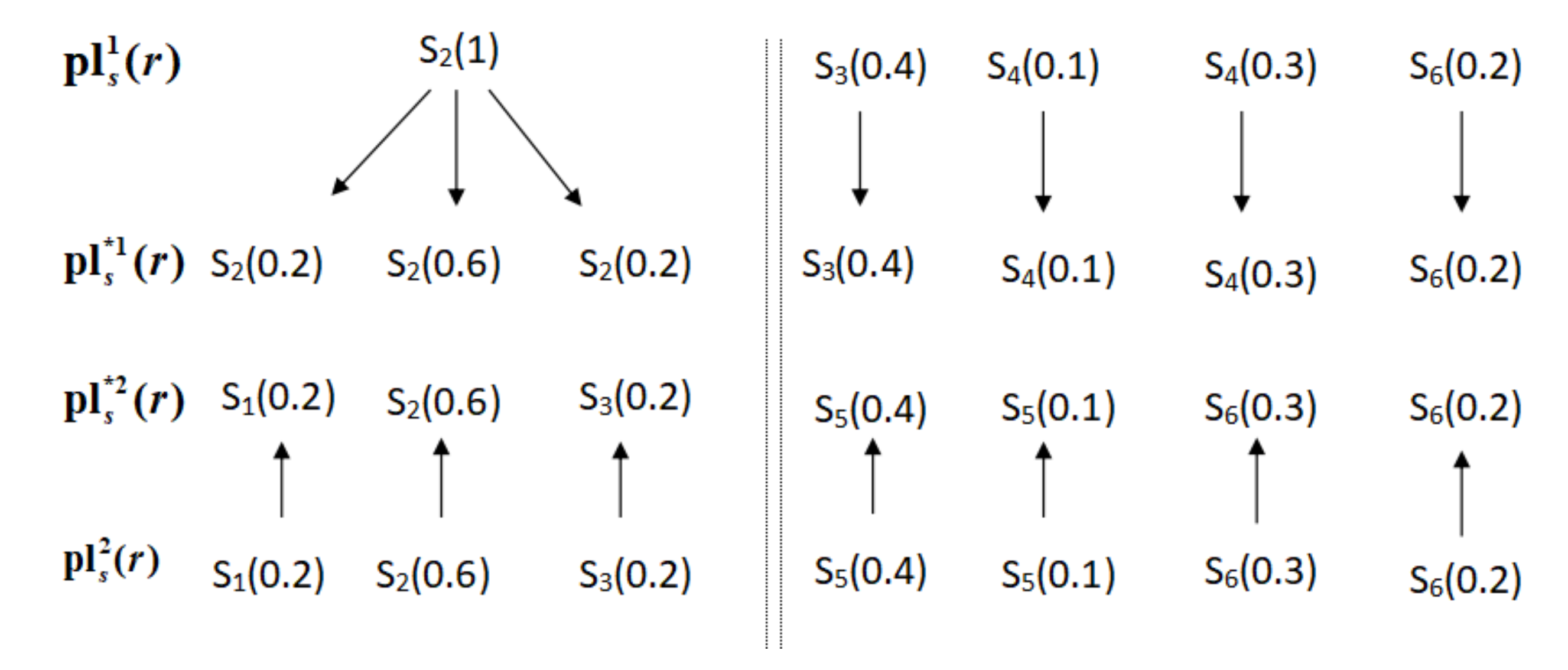
Example 1.

Let $S=\{s_0:veryslowly,s_1:slowly,s_2:slightlyslowly,s_3:generally,s_4:slightlyfast,s_5:fast,s_6:veryfast\}$. Two groups of experts inspected the development of the company, one group may think that “the speed of company development is slightly slowly with 100% possibility, with 40% probability that it is not slightly slowly, with 40% probability that the speed of company development is not generally and with 20% probability that the speed of company development is not slightly fast”. The other group think that “with 20% probability that the speed of company development is slowly, with 60% probability that the speed of company development is slightly slowly and with 20% probability that it is generally, with 50% probability that it is not slightly fast and with 50% probability that it is not very fast”. Then the above evaluation information can be denoted as $p{l}_s^1(r)=⟨\{s_2(1)\},\{s_2(0.4),s_3(0.4),s_4(0.2)\}⟩$ and $p{l}_s^2(r)=⟨\{s_1(0.2),s_2(0.6),s_3(0.2)\},\{s_5(0.5),s_6(0.5)\}⟩$.

According to Example 1, we can see that the probabilities and numbers of elements in $p{l}_s^1(r)$ and $p{l}_s^2(r)$ are not same, the general operations on PLFSs multiply the probabilities of corresponding linguistic terms directly, which may cause the unreasonable result. Therefore, Wu et al. [26] presented a method to modify the probabilities of linguistic terms to be same, which is given as follows:

Let ${\overline{S}}_{[0,\rho ]}(\rho >2g)$ be a continuous LTS, $p{l}_s^1(r)=⟨\{s_{{\theta }^{1(u)}}({\widehat{r}}^{(u)})\},\{s_{{\varphi }^{1(v)}}({\tilde{r}}^{(v)})\}|u=1,2,\cdots ,U_1;v=1,2,\cdots ,V_1⟩$ and $p{l}_s^2(r)=⟨\{s_{{\theta }^{2(u)}}({\widehat{r}}^{(u)})\},\{s_{{\varphi }^{2(v)}}({\tilde{r}}^{(v)})\}|u=1,2,\cdots ,U_2$; $v=1,2,\cdots ,V_2⟩$ are two PLQRONs. We adjust the probability distributions of $p{l}_s^1(r)$ and $p{l}_s^2(r)$ to be same, respectively. That is to say, $p{l}_s^{\ast 1}(r)=⟨\{s_{{\theta }^{1(k)}}({\widehat{r}}^{\ast (k)})\},\{s_{{\varphi }^{1(b)}}({\tilde{r}}^{\ast (b)})\}|k=1,2,\cdots ,K;b=1,2,\cdots ,B⟩$ and $p{l}_s^{\ast 2}(r)=⟨\{s_{{\theta }^{2(k)}}({\widehat{r}}^{\ast (k)})\},\{s_{{\varphi }^{2(b)}}({\tilde{r}}^{\ast (b)})\}|k=1,2,\cdots ,K$; $b=1,2,\cdots ,B⟩$. Applying the method of Wu et al. [26] to adjust the PLQRONs, the linguistic terms and the sum of probabilities of each linguistic term set are not changed, which means that the adjustment method does not result in the loss of evaluation information.

Example 2.

Let $S=\{s_{\alpha }|\alpha =0,1,2,\cdots ,6\}$, $p{l}_s^1(r)=⟨\{s_2(1)\},\{s_3(0.4),s_4(0.4),s_6(0.2)\}⟩$ and $p{l}_s^2(r)=⟨\{s_1(0.2),s_2(0.6),s_3(0.2)\},\{s_5(0.5),s_6(0.5)\}⟩$ be two PLQRONs, the adjusted PLQRONs are $p{l}_s^{\ast 1}(r)=⟨\{s_2(0.2)$, $s_2(0.6),s_2(0.2)\},\{s_3(0.4),s_4(0.1),s_4(0.3),s_6(0.2)\}⟩$ and $p{l}_s^{\ast 2}(r)=⟨\{s_1(0.2),s_2(0.6),s_3(0.2)\},\{s_5(0.4),s_5(0.1),s_6(0.3),s_6(0.2)\}⟩$, respectively. The adjustment process is shown in Figure 1.

Figure 1. The adjust process of PLQRONs $p{l}_s^1(r)$ and $p{l}_s^2(r)$.

3.2. Some Properties for PLQRONs

Firstly, we apply the adjustment method to adjust the probabilistic linguistic terms with same probability, which can overcome the defects that may occur in process of aggregation. Then, we propose the operation rules of the adjusted PLQRONs, and their properties.

Definition 7.

Let ${\overline{S}}_{[0,\rho ]}(\rho >2g)$ be a LTS, $p{l}_s^{\ast 1}(r)=⟨\{s_{{\theta }^{1(u)}}({\widehat{r}}^{\ast (u)})\},\{s_{{\varphi }^{1(v)}}({\tilde{r}}^{\ast (v)})\}⟩$ and $p{l}_s^{\ast 2}(r)=⟨\{s_{{\theta }^{2(u)}}({\widehat{r}}^{\ast (u)})\},$$\{s_{{\varphi }^{2(v)}}({\tilde{r}}^{\ast (v)})\}⟩$$(u=1,2,\cdots ,U;v=1,2,\cdots ,V)$ are two adjusted PLQRONs, where ${\theta }^{\iota (u)},{\varphi }^{\iota (v)}(\iota =1,2)$ are the subscript of $s_{{\theta }^{\iota (u)}},s_{{\varphi }^{\iota (v)}}(\iota =1,2),\eta >0$, the operational laws of the PLQRONs can be expressed as follows:

(a) 

$neg(p{l}_s^{\ast 1}(r))=⟨\{s_{{\varphi }^{1(v)}}({\tilde{r}}^{\ast (v)})\},\{s_{{\theta }^{1(u)}}({\widehat{r}}^{\ast (u)})\}⟩$;

(b) 

$p{l}_s^{\ast 1}(r)\oplus p{l}_s^{\ast 2}(r)=⟨\{s_{{({({\theta }^{1(u)})}^q+{({\theta }^{2(u)})}^q-{(\frac{({\theta }^{1(u)})({\theta }^{2(u)})}{\rho })}^q)}^{\frac{1}{q}}}({\widehat{r}}^{\ast (u)})\},\{s_{\frac{{\varphi }^{1(v)}{\varphi }^{2(v)}}{\rho }}({\tilde{r}}^{\ast (v)})\}⟩$;

(c) 

$p{l}_s^{\ast 1}(r)\otimes p{l}_s^{\ast 2}(r)=⟨\{s_{\frac{{\theta }^{1(u)}{\theta }^{2(u)}}{\rho }}({\widehat{r}}^{\ast (u)})\},\{s_{{({({\varphi }^{1(v)})}^q+{({\varphi }^{2(v)})}^q-{(\frac{({\varphi }^{1(v)})({\varphi }^{2(v)})}{\rho })}^q)}^{\frac{1}{q}}}({\tilde{r}}^{\ast (v)})\}⟩$;

(d) 

$\eta p{l}_s^{\ast 1}(r)=⟨\{s_{{({\rho }^q-{\rho }^q{(1-\frac{{({\theta }^{1(u)})}^q}{{\rho }^q})}^{\eta })}^{\frac{1}{q}}}({\widehat{r}}^{\ast (u)})\},\{s_{\rho {(\frac{{\varphi }^{1(v)}}{\rho })}^{\eta }}({\tilde{r}}^{\ast (v)})\}⟩$;

(e) 

${(p{l}_s^{\ast 1}(r))}^{\eta }=⟨\{s_{\rho {(\frac{{\theta }^{1(u)}}{\rho })}^{\eta }}({\widehat{r}}^{\ast (u)})\},\{s_{{({\rho }^q-{\rho }^q{(1-\frac{{({\varphi }^{1(v)})}^q}{{\rho }^q})}^{\eta })}^{\frac{1}{q}}}({\tilde{r}}^{\ast (v)})\}⟩$.

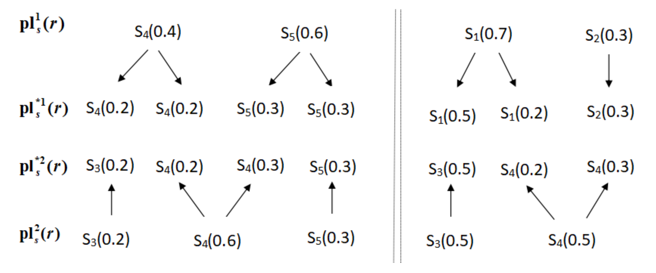
Example 3.

Let $S=\{s_{\alpha }|\alpha =0,1,2,\cdots ,6\}$, $p{l}_s^1(r)=⟨\{s_4(0.4),s_5(0.6)\},\{s_1(0.7),s_2(0.3)\}⟩$ and $p{l}_s^2(r)=⟨\{s_3(0.2),s_4(0.5),s_5(0.3)\},\{s_3(0.5),s_4(0.5)\}⟩$ be two PLQRONs, the modified PLQRONs are $p{l}_s^{\ast 1}(r)=⟨\{s_4(0.2),s_4(0.2),s_5(0.3),s_5(0.3)\},\{s_1(0.5),s_1(0.2),s_2(0.3)\}⟩$ and $p{l}_s^{\ast 2}(r)=⟨\{s_3(0.2),s_4(0.2),s_4(0.3),s_5(0.3)\},\{s_3(0.5),s_4(0.2),s_4(0.3)\}⟩$, The adjustment process is shown in Figure 2. Let $\eta =0.5$ and $q=3$, then we have

$$\begin{array}{cc}\hfill & neg(p{l}_s^{\ast 1}(r))=⟨\{s_1(0.5),s_1(0.2),s_2(0.3)\},\{s_4(0.2),s_4(0.2),s_5(0.3),s_5(0.3)\}⟩;\hfill \\ \hfill & p{l}_s^{\ast 1}(r)\oplus p{l}_s^{\ast 2}(r)=⟨\{s_{4.3621}(0.2),s_{4.7774}(0.2),s_{5.3364}(0.3),s_{5.6217}(0.3)\},\{s_{0.5}(0.5),s_{0.6667}(0.2),s_{1.3333}(0.3)\}⟩;\hfill \\ \hfill & p{l}_s^{\ast 1}(r)\otimes p{l}_s^{\ast 2}(r)=⟨\{s_2(0.2),s_{2.6667}(0.2),s_{3.3333}(0.3),s_{4.1667}(0.3)\},\{s_{3.0321}(0.5),s_{4.0146}(0.2),s_{4.114}(0.3)\}⟩;\hfill \\ \hfill & 0.5p{l}_s^{\ast 1}(r)=⟨\{s_{3.2649}(0.2),s_{3.2649}(0.2),s_{4.2321}(0.3),s_{4.2321}(0.3)\},\{s_{2.4495}(0.5),s_{2.4495}(0.2),s_{3.4641}(0.3)\}⟩;\hfill \\ \hfill & {(p{l}_s^{\ast 1}(r))}^{0.5}=⟨\{s_{4.899}(0.2),s_{4.899}(0.2),s_{5.4772}(0.3),s_{5.4772}(0.3)\},\{s_{0.794}(0.5),s_{0.794}(0.2),s_{1.5924}(0.3)\}⟩.\hfill \end{array}$$

Figure 2. The adjust process of PLQRONs $p{l}_s^1(r)$ and $p{l}_s^2(r)$.

Theorem 1.

Let $p{l}_s^{\ast 1}(r)=⟨\{s_{{\theta }^{1(u)}}({\widehat{r}}^{\ast (u)})\},\{s_{{\varphi }^{1(v)}}({\tilde{r}}^{\ast (v)})\}⟩$ and $p{l}_s^{\ast 2}(r)=⟨\{s_{{\theta }^{2(u)}}({\widehat{r}}^{\ast (u)})\}$, $\{s_{{\varphi }^{2(v)}}({\tilde{r}}^{\ast (v)})\}⟩$$(u=1,2,\cdots ,U;v=1,2,\cdots ,V)$ be any two adjusted PLQRONs, $\eta ,{\eta }_1,{\eta }_2>0$, then

(1) 

$p{l}_s^{\ast 1}(r)\oplus p{l}_s^{\ast 2}(r)=p{l}_s^{\ast 2}(r)\oplus p{l}_s^{\ast 1}(r)$;

(2) 

$p{l}_s^{\ast 1}(r)\otimes p{l}_s^{\ast 2}(r)=p{l}_s^{\ast 2}(r)\otimes p{l}_s^{\ast 1}(r)$;

(3) 

$\eta (p{l}_s^{\ast 1}(r)\oplus p{l}_s^{\ast 2}(r))=\eta p{l}_s^{\ast 1}(r)\oplus \eta p{l}_s^{\ast 2}(r)$;

(4) 

${\eta }_{1}p{l}_s^{\ast 1}(r)\oplus {\eta }_{2}p{l}_s^{\ast 1}(r)=({\eta }_1+{\eta }_2)p{l}_s^{\ast 1}(r)$;

(5) 

${(p{l}_s^{\ast 1}(r))}^{{\eta }_1}\otimes {(p{l}_s^{\ast 1}(r))}^{{\eta }_2}={(p{l}_s^{\ast 1}(r))}^{{\eta }_1+{\eta }_2}$;

(6) 

${(p{l}_s^{\ast 1}(r))}^{\eta }\otimes {(p{l}_s^{\ast 2}(r))}^{\eta }={(p{l}_s^{\ast 1}(r)\otimes p{l}_s^{\ast 2}(r))}^{\eta }$.

Here we prove the property (1) and (3), other properties proof process are similar, we omit them.

(1)

By Definition 7, we have

$$\begin{array}{c}\hfill \begin{array}{cc}\hfill p{l}_s^{\ast 1}(r)\oplus p{l}_s^{\ast 2}(r)& =⟨\{s_{{({({\theta }^{1(u)})}^q+{({\theta }^{2(u)})}^q-{(\frac{({\theta }^{1(u)})({\theta }^{2(u)})}{\rho })}^q)}^{\frac{1}{q}}}({\widehat{r}}^{\ast (u)})\},\{s_{\frac{{\varphi }^{1(v)}{\varphi }^{2(v)}}{\rho }}({\tilde{r}}^{\ast (v)})\}⟩\hfill \\ \hfill & =⟨\{s_{{({({\theta }^{2(u)})}^q+{({\theta }^{1(u)})}^q-{(\frac{({\theta }^{2(u)})({\theta }^{1(u)})}{\rho })}^q)}^{\frac{1}{q}}}({\widehat{r}}^{\ast (u)})\},\{s_{\frac{{\varphi }^{2(v)}{\varphi }^{1(v)}}{\rho }}({\tilde{r}}^{\ast (v)})\}⟩\hfill \\ \hfill & =p{l}_s^{\ast 2}(r)\oplus p{l}_s^{\ast 1}(r).\hfill \end{array}\end{array}$$

Therefore $p{l}_s^{\ast 1}(r)\oplus p{l}_s^{\ast 2}(r)=p{l}_s^{\ast 2}(r)\oplus p{l}_s^{\ast 1}(r)$ is obtained.

(3)

By Definition 7, we can get

$$\begin{array}{c}\hfill \begin{array}{cc}\hfill \eta (p{l}_s^{\ast 1}(r)\oplus p{l}_s^{\ast 2}(r))& =\eta ⟨\{s_{{({({\theta }^{1(u)})}^q+{({\theta }^{2(u)})}^q-{(\frac{{\theta }^{1(u)}{\theta }^{2(u)}}{\rho })}^q)}^{\frac{1}{q}}}({\widehat{r}}^{\ast (u)})\},\{s_{\frac{{\varphi }^{1(v)}{\varphi }^{2(v)}}{\rho }}({\tilde{r}}^{\ast (v)})\}⟩\hfill \\ \hfill & =⟨\{s_{{({\rho }^q-{\rho }^q{(1-\frac{{({\theta }^{1(u)})}^q+{({\theta }^{2(u)})}^q-{(\frac{({\theta }^{1(u)})({\theta }^{2(u)})}{\rho })}^q}{{\rho }^q})}^{\eta })}^{\frac{1}{q}}}({\widehat{r}}^{\ast (u)})\},\{s_{\rho {(\frac{{\varphi }^{1(v)}{\varphi }^{2(v)}}{{\rho }^2})}^{\eta }}({\tilde{r}}^{\ast (v)})\}⟩.\hfill \end{array}\end{array}$$

Moreover, since

$$\begin{array}{c}\eta (p{l}_s^{\ast 1}(r))=⟨\{s_{{({\rho }^q-{\rho }^q{(1-\frac{{({\theta }^{1(u)})}^q}{{\rho }^q})}^{\eta })}^{\frac{1}{q}}}({\widehat{r}}^{\ast (u)})\},\{s_{\rho {(\frac{{\varphi }^{1(v)}}{\rho })}^{\eta }}({\tilde{r}}^{\ast (v)})\}⟩,\\ \eta (p{l}_s^{\ast 2}(r))=⟨\{s_{{({\rho }^q-{\rho }^q{(1-\frac{{({\theta }^{2(u)})}^q}{{\rho }^q})}^{\eta })}^{\frac{1}{q}}}({\widehat{r}}^{\ast (u)})\},\{s_{\rho {(\frac{{\varphi }^{2(v)}}{\rho })}^{\eta }}({\tilde{r}}^{\ast (v)})\}⟩,\end{array}$$

let $\varpi ={({\rho }^q-{\rho }^q{(1-\frac{{({\theta }^{1(u)})}^q}{{\rho }^q})}^{\eta })}^{\frac{1}{q}}$ and $\chi ={({\rho }^q-{\rho }^q{(1-\frac{{({\theta }^{2(u)})}^q}{{\rho }^q})}^{\eta })}^{\frac{1}{q}}$, the above formulas can be denoted as:

$$\begin{array}{cc}\hfill & \eta p{l}_s^{\ast 1}(r)\oplus \eta p{l}_s^{\ast 2}(r)=⟨\{s_{{({\varpi }^q+{\chi }^q-{(\frac{\varpi ·\chi }{\rho })}^q)}^{1/q}}({\widehat{r}}^{\ast (u)})\},\{s_{\rho {(\frac{{\varphi }^{1(v)}{\varphi }^{2(v)}}{{\rho }^2})}^{\eta }}({\tilde{r}}^{\ast (v)})\}⟩\hfill \\ \hfill & =⟨\{s_{{\{{\rho }^q-{\rho }^q·[{(1-\frac{{({\theta }^{1(u)})}^q}{{\rho }^q})}^{\eta }+{(1-\frac{{({\theta }^{2(u)})}^q}{{\rho }^q})}^{\eta }]-(1-{(1-\frac{{({\theta }^{1(u)})}^q}{{\rho }^q})}^{\eta })·[{\rho }^q-{\rho }^q{(1-\frac{{({\theta }^{2(u)})}^q}{{\rho }^q})}^{\eta }]\}}^{\frac{1}{q}}}({\widehat{r}}^{\ast (u)})\},\{s_{\rho {(\frac{{\varphi }^{1(v)}{\varphi }^{2(v)}}{{\rho }^2})}^{\eta }}({\tilde{r}}^{\ast (v)})\}⟩\hfill \\ \hfill & =⟨\{s_{{\{{\rho }^q-{\rho }^q·[{(1-\frac{{({\theta }^{1(u)})}^q}{{\rho }^q})}^{\eta }+{(1-\frac{{({\theta }^{2(u)})}^q}{{\rho }^q})}^{\eta }]+{\rho }^q[{(1-\frac{{({\theta }^{1(u)})}^q}{{\rho }^q})}^{\eta }+{(1-\frac{{({\theta }^{2(u)})}^q}{{\rho }^q})}^{\eta }-{(1-\frac{{({\theta }^{1(u)})}^q}{{\rho }^q})}^{\eta }·{(1-\frac{{({\theta }^{2(u)})}^q}{{\rho }^q})}^{\eta }]\}}^{\frac{1}{q}}}({\widehat{r}}^{\ast (u)})\},\hfill \\ & \{s_{\rho {(\frac{{\varphi }^{1(v)}{\varphi }^{2(v)}}{{\rho }^2})}^{\eta }}({\tilde{r}}^{\ast (v)})\}⟩\hfill \\ \hfill & =⟨\{s_{{\{{\rho }^q-{\rho }^q·[{(1-\frac{{({\theta }^{1(u)})}^q}{{\rho }^q})}^{\eta }·{(1-\frac{{({\theta }^{2(u)})}^q}{{\rho }^q})}^{\eta }]\}}^{\frac{1}{q}}}({\widehat{r}}^{\ast (u)})\},\{s_{\rho {(\frac{{\varphi }^{1(v)}{\varphi }^{2(v)}}{{\rho }^2})}^{\eta }}({\tilde{r}}^{\ast (v)})\}⟩\hfill \\ \hfill & =⟨\{s_{{({\rho }^q-{\rho }^q{(1-\frac{{({\theta }^{1(u)})}^q+{({\theta }^{2(u)})}^q-{(\frac{({\theta }^{1(u)})({\theta }^{2(u)})}{\rho })}^q}{{\rho }^q})}^{\eta })}^{\frac{1}{q}}}({\widehat{r}}^{\ast (u)})\},\{s_{\rho {(\frac{{\varphi }^{1(v)}{\varphi }^{2(v)}}{{\rho }^2})}^{\eta }}({\tilde{r}}^{\ast (v)})\}⟩\hfill \\ \hfill & =\eta (p{l}_s^{\ast 1}(r)\oplus p{l}_s^{\ast 2}(r)).\hfill \end{array}$$

Therefore $\eta (p{l}_s^{\ast 1}(r)\oplus p{l}_s^{\ast 2}(r))=\eta p{l}_s^{\ast 1}(r)\oplus \eta p{l}_s^{\ast 2}(r)$ is proved.

In order to compare the order relation of PLQROSs, we present the comparison rules as follows:

Definition 8.

Assume ${\overline{S}}_{[0,\rho ]}(\rho >2g)$ be a LTS, for any adjusted PLQRON $p{l}_s^{\ast }(r)=⟨\{s_{{\theta }^{(u)}}({\widehat{r}}^{\ast (u)})\}$, $\{s_{{\varphi }^{(v)}}({\tilde{r}}^{\ast (v)})\}⟩$, where $s_{{\theta }^{(u)}},s_{{\varphi }^{(v)}}\in {\tilde{S}}_{[0,\rho ]},(u=1,2,\cdots ,U;v=1,2,\cdots ,V)$, the score function of $p{l}_s^{\ast }(r)$ is

$$A(p{l}_s^{\ast }(r))=\sum _{u=1}^{\#U_{\theta }}{(\frac{{\theta }^{(u)}·{\widehat{r}}^{\ast (u)}}{\rho })}^q-\sum _{v=1}^{\#V_{\varphi }}{(\frac{{\varphi }^{(v)}·{\tilde{r}}^{\ast (v)}}{\rho })}^q,$$

(1)

where ${\theta }^{(u)},{\varphi }^{(v)}\in [0,\rho ]$, $\#U_{\theta }$ and $\#V_{\varphi }$ represent the number of elements in the corresponding set, respectively.

The accuracy function of $p{l}_s^{\ast }(r)$ is

$$H(p{l}_s^{\ast }(r))=\sum _{u=1}^{\#U_{\theta }}{(\frac{{\theta }^{(u)}·{\widehat{r}}^{\ast (u)}}{\rho })}^q+\sum _{v=1}^{\#V_{\varphi }}{(\frac{{\varphi }^{(v)}·{\tilde{r}}^{\ast (v)}}{\rho })}^q,$$

(2)

where ${\theta }^{(u)},{\varphi }^{(v)}\in [0,\rho ]$, $\#U_{\theta }$ and $\#V_{\varphi }$ represent the number of elements in the corresponding set, respectively.

Theorem 2.

Let $p{l}_s^{\ast 1}(r)=⟨\{s_{{\theta }^{1(u)}}({\widehat{r}}^{\ast (u)})\},\{s_{{\varphi }^{1(v)}}({\tilde{r}}^{\ast (v)})\}⟩$ and $p{l}_s^{\ast 2}(r)=⟨\{s_{{\theta }^{2(u)}}({\widehat{r}}^{\ast (u)})\}$, $\{s_{{\varphi }^{2(v)}}({\tilde{r}}^{\ast (v)})\}⟩$ be two adjusted PLQRONs. $A(p{l}_s^{\ast 1}(r))$ and $A(p{l}_s^{\ast 2}(r))$ are the score function of $p{l}_s^{\ast 1}(r)$ and $p{l}_s^{\ast 2}(r)$, the accuracy function of $p{l}_s^{\ast 1}(r)$ and $p{l}_s^{\ast 2}(r)$ are $H(p{l}_s^{\ast 1}(r))$ and $H(p{l}_s^{\ast 2}(r))$, respectively, then the order relation of $p{l}_s^{\ast 1}(r)$ and $p{l}_s^{\ast 2}(r)$ are given as follows:

(1) 

If $A(p{l}_s^{\ast 1}(r))>A(p{l}_s^{\ast 2}(r))$, then $p{l}_s^{\ast 1}(r)\succ p{l}_s^{\ast 2}(r)$;

(2) 

If $A(p{l}_s^{\ast 1}(r))=A(p{l}_s^{\ast 2}(r))$, then

(a) 

If $H(p{l}_s^{\ast 1}(r))=H(p{l}_s^{\ast 2}(r))$, then $p{l}_s^{\ast 1}(r)\asymp p{l}_s^{\ast 2}(r)$;

(b) 

If $H(p{l}_s^{\ast 1}(r))<H(p{l}_s^{\ast 2}(r))$, then $p{l}_s^{\ast 1}(r)\prec p{l}_s^{\ast 2}(r)$;

(c) 

If $H(p{l}_s^{\ast 1}(r))>H(p{l}_s^{\ast 2}(r))$, then $p{l}_s^{\ast 1}(r)\succ p{l}_s^{\ast 2}(r)$;

(3) 

If $A(p{l}_s^{\ast 1}(r))<A(p{l}_s^{\ast 2}(r))$, then $p{l}_s^{\ast 1}(r)\prec p{l}_s^{\ast 2}(r)$.

3.3. The Aggregation Operators of PLQROSs

In order to aggregate the multi-attribute information well, we introduce the aggregation operators of PLQRONs as follows.

Definition 9.

Let ${\overline{S}}_{[0,\rho ]}(\rho >2g)$ be a LTS, $p{l}_s^{\ast 1}(r)=⟨\{s_{{\theta }^{\iota (u)}}({\widehat{r}}^{\ast (u)})\},\{s_{{\varphi }^{\iota (v)}}({\tilde{r}}^{\ast (v)})\}⟩(\iota =1,2,\cdots ,n;u=1,2,\cdots ,U;v=1,2,\cdots ,V)$ are n adjusted PLQRONs, where $s_{{\theta }^{\iota (u)}},s_{{\varphi }^{\iota (v)}}\in {\overline{S}}_{[0,\rho ]}$, the probabilistic linguistic q-rung orthopair weighted averaging (PLQROWA) operator can be expressed as:

$$\begin{array}{c}\hfill \begin{array}{cc}\hfill PLQROWA(p{l}_s^{\ast 1}(r),p{l}_s^{\ast 2}(r),\cdots ,p{l}_s^{\ast n}(r))& ={\omega }_{1}p{l}_s^{\ast 1}(r)\oplus {\omega }_{2}p{l}_s^{\ast 2}(r)\oplus \cdots \oplus {\omega }_{n}p{l}_s^{\ast n}(r)\hfill \\ & =⟨\{s_{{({\rho }^q-{\rho }^q{\prod }_{\iota =1}^n{(1-\frac{{({\theta }^{\iota (u)})}^q}{{\rho }^q})}^{{\omega }_{\iota }})}^{\frac{1}{q}}}({\widehat{r}}^{\ast (u)})\},\{s_{{\prod }_{\iota =1}^n\rho {(\frac{{\varphi }^{\iota (v)}}{\rho })}^{{\omega }_{\iota }}}({\tilde{r}}^{\ast (v)})\}⟩,\hfill \end{array}\end{array}$$

(3)

where $\omega ={({\omega }_1,{\omega }_2,\cdots ,{\omega }_n)}^T$ is the weight vector, and it satisfies ${\sum }_{\iota =1}^n{\omega }_{\iota }=1(0\le {\omega }_{\iota }\le 1)$.

Theorem 3.

Let $p{l}_s^{\ast \iota }(r)=⟨\{s_{{\theta }^{\iota (u)}}({\widehat{r}}^{\ast (u)})\},\{s_{{\varphi }^{\iota (v)}}({\tilde{r}}^{\ast (v)})\}⟩(\iota =1,2,\cdots ,n;u=1,2,\cdots ,U$; $v=1,2,\cdots ,V)$ be ι adjusted PLQRONs, the weight ${\omega }_{\iota }(\iota =1,2,\cdots ,n)$ satisfies with $0\le {\omega }_{\iota }\le 1$ and ${\sum }_{\iota =1}^n{\omega }_{\iota }=1$, then the properties of PLQROWA are shown as follows:

(1) 

Idempotency: if $p{l}_s^{\ast \iota }(r)(\iota =1,2,\cdots ,n)$ are equal, i.e., $p{l}_s^{\ast \iota }(r)=p{l}_s^{\ast }(r)\triangleq ⟨\{s_{{\theta }^{(u)}}({\widehat{r}}^{\ast (u)})\},\{s_{{\varphi }^{(v)}}({\tilde{r}}^{\ast (v)})\}⟩$, then

$$PLQROWA(p{l}_s^{\ast 1}(r),p{l}_s^{\ast 2}(r),\cdots ,p{l}_s^{\ast n}(r))=p{l}_s^{\ast }(r)=⟨\{s_{{\theta }^{(u)}}({\widehat{r}}^{\ast (u)})\},\{s_{{\varphi }^{(v)}}({\tilde{r}}^{\ast (v)})\}⟩.$$

(2) 

Monotonicity: let $p{l}_s^{\ast 1}(r),p{l}_s^{\ast 2}(r),\cdots ,p{l}_s^{\ast n}(r)$ and $p{l}_s^{{}^{\prime }\ast 1}(r),p{l}_s^{{}^{\prime }\ast 2}(r),\cdots ,p{l}_s^{{}^{\prime }\ast n}(r)$ be two collections of adjusted PLQRONs, for all ι, $s_{{\theta }^{\iota (u)}}<{s^{\prime }}_{{\theta }^{\iota (u)}}$ and $s_{{\varphi }^{\iota (v)}}>{s^{\prime }}_{{\varphi }^{\iota (v)}}$, then

$$PLQROWA(p{l}_s^{\ast 1}(r),p{l}_s^{\ast 2}(r),\cdots ,p{l}_s^{\ast n}(r))<PLQROWA(p{l}_s^{{}^{\prime }\ast 1}(r),p{l}_s^{{}^{\prime }\ast 2}(r),\cdots ,p{l}_s^{{}^{\prime }\ast n}(r)).$$

(3) 

Boundedness: let $s_{{\theta }^{\iota (+)}}=\underset{u=1}{\overset{U}{max}}{s}_{{\theta }^{\iota (u)}}$, $s_{{\theta }^{\iota (-)}}=\underset{u=1}{\overset{U}{min}}{s}_{{\theta }^{\iota (u)}}$, $s_{{\varphi }^{\iota (+)}}=\underset{v=1}{\overset{V}{max}}{s}_{{\varphi }^{\iota (v)}}$ and $s_{{\varphi }^{\iota (-)}}=\underset{v=1}{\overset{V}{min}}{s}_{{\varphi }^{\iota (v)}}$, then

$$⟨\{s_{{\theta }^{\iota (-)}}({\widehat{r}}^{\ast (u)})\},\{s_{{\varphi }^{\iota (+)}}({\tilde{r}}^{\ast (v)})\}⟩\le PLQROWA(p{l}_s^{\ast 1}(r),p{l}_s^{\ast 2}(r),\cdots ,p{l}_s^{\ast n}(r))\le ⟨\{s_{{\theta }^{\iota (+)}}({\widehat{r}}^{\ast (u)})\},\{s_{{\varphi }^{\iota (-)}}({\tilde{r}}^{\ast (v)})\}⟩.$$

(1)

For all $\iota$, since $p{l}_s^{\ast \iota }(r)=p{l}_s^{\ast }(p)=⟨\{s_{{\theta }^{(u)}}({\widehat{r}}^{\ast (u)})\},\{s_{{\varphi }^{(v)}}({\tilde{r}}^{\ast (v)})\}⟩$, then

$$\begin{array}{c}\hfill \begin{array}{cc}\hfill PLQROWA(p{l}_s^{\ast 1}(r),p{l}_s^{\ast 2}(r),\cdots ,p{l}_s^{\ast n}(r))& ={\omega }_{1}p{l}_s^{\ast 1}(r)\oplus {\omega }_{2}p{l}_s^{\ast 2}(r)\oplus \cdots \oplus {\omega }_{n}p{l}_s^{\ast n}(r)\hfill \\ & =⟨\{s_{{({\rho }^q-{\rho }^q{\prod }_{\iota =1}^n{(1-\frac{{({\theta }^{\iota (u)})}^q}{{\rho }^q})}^{{\omega }_{\iota }})}^{\frac{1}{q}}}({\widehat{r}}^{\ast (u)})\},\{s_{{\prod }_{\iota =1}^n\rho {(\frac{{\varphi }^{\iota (v)}}{\rho })}^{{\omega }_{\iota }}}({\tilde{r}}^{\ast (v)})\}⟩\hfill \\ \hfill & =⟨\{s_{{({\rho }^q-{\rho }^q{(1-\frac{{({\theta }^{\iota (u)})}^q}{{\rho }^q})}^{{\sum }_{\iota =1}^n{\omega }_{\iota }})}^{\frac{1}{q}}}({\widehat{r}}^{\ast (u)})\},\{s_{\rho {(\frac{{\varphi }^{\iota (v)}}{\rho })}^{{\sum }_{\iota =1}^n{\omega }_{\iota }}}({\tilde{r}}^{\ast (v)})\}⟩\hfill \\ \hfill & =⟨\{s_{{({\rho }^q-{\rho }^q(1-\frac{{({\theta }^{(u)})}^q}{{\rho }^q}))}^{\frac{1}{q}}}({\widehat{r}}^{\ast (u)})\},\{s_{\rho (\frac{{\varphi }^{(v)}}{\rho })}({\tilde{r}}^{\ast (v)})\}⟩\hfill \\ \hfill & =⟨\{s_{{\theta }^{(u)}}({\widehat{r}}^{\ast (u)})\},\{s_{{\varphi }^{(v)}}({\tilde{r}}^{\ast (v)})\}⟩.\hfill \end{array}\end{array}$$

Therefore $PLQROWA(p{l}_s^{\ast 1}(r),p{l}_s^{\ast 2}(r),\cdots ,p{l}_s^{\ast n}(r))=⟨\{s_{{\theta }^{(u)}}({\widehat{r}}^{\ast (u)})\},\{s_{{\varphi }^{(v)}}({\tilde{r}}^{\ast (v)})\}⟩$ is proved.

(2)

For all $\iota$, $s_{{\theta }^{\iota (u)}}<{s^{\prime }}_{{\theta }^{\iota (u)}}$ and $s_{{\varphi }^{\iota (v)}}>{s^{\prime }}_{{\varphi }^{\iota (v)}}$, then we have

$${s^{\prime }}_{1-\frac{{\theta }^{\iota (u)}}{\rho }}<s_{1-\frac{{\theta }^{\iota (u)}}{\rho }}\Rightarrow s_{{(\rho -\rho {\prod }_{\iota =1}^n{(1-{(\frac{{\theta }^{\iota (u)}}{\rho })}^q)}^{{\omega }_{\iota }})}^{\frac{1}{q}}}<{s^{\prime }}_{{(\rho -\rho {\prod }_{\iota =1}^n{(1-{(\frac{{\theta }^{\iota (u)}}{\rho })}^q)}^{{\omega }_{\iota }})}^{\frac{1}{q}}},s_{{\prod }_{\iota =1}^n{({\varphi }^{\iota (v)})}^{{\omega }_{\iota }}}>{s^{\prime }}_{{\prod }_{\iota =1}^n{({\varphi }^{\iota (v)})}^{{\omega }_{\iota }}}.$$

Assume $PLQROWA(p{l}_s^{\ast 1}(r),p{l}_s^{\ast 2}(r),\cdots ,p{l}_s^{\ast n}(r))=p{l}_s(r)$ and $PLQROWA(p{l}_s^{{}^{\prime }\ast 1}(r)$, $p{l}_s^{{}^{\prime }\ast 2}(r),\cdots ,p{l}_s^{{}^{\prime }\ast n}(r))=p{l}_s^{\prime }(r)$, by (1), we can get

$$A(p{l}_s^{\ast }(r))=\sum _{u=1}^{\#U_{\theta }}{({\displaystyle \frac{{(\rho -\rho ·{\prod }_{\iota =1}^n{(1-{(\frac{{\theta }^{(u)}}{\rho })}^q)}^{{\omega }_{\iota }})}^{\frac{1}{q}}}{\rho }}·({\widehat{r}}^{\ast (u)}))}^q-\sum _{v=1}^{\#V_{\varphi }}{(\frac{{({\varphi }^{(v)})}^{{\omega }_{\iota }}}{\rho }·{\tilde{r}}^{\ast (v)})}^q;$$

$$A(p{l}_s^{{}^{\prime }\ast }(r))=\sum _{u=1}^{\#U_{{\theta }^{{}^{\prime }}}}{({\displaystyle \frac{{(\rho -\rho ·{\prod }_{\iota =1}^n{(1-{(\frac{{\theta }^{\prime (u)}}{\rho })}^q)}^{{\omega }_{\iota }})}^{\frac{1}{q}}}{\rho }}·({\widehat{r^{\prime }}}^{\ast (u)}))}^q-\sum _{v=1}^{\#V_{{\varphi }^{{}^{\prime }}}}{(\frac{{({\varphi }^{\prime (v)})}^{{\omega }_{\iota }}}{\rho }·{\widetilde{r^{\prime }}}^{\ast (v)})}^q.$$

Then we have $A(p{l}_s^{\ast }(r))<A(p{l}_s^{{}^{\prime }\ast }(r))$, that is $p{l}_s^{\ast }(r)<p{l}_s^{{}^{\prime }\ast }(r)$.

Therefore $PLQROWA(p{l}_s^{\ast 1}(r),p{l}_s^{\ast 2}(r),\cdots ,p{l}_s^{\ast n}(r))<PLQROWA(p{l}_s^{{}^{\prime }\ast 1}(r),p{l}_s^{{}^{\prime }\ast 2}(r)$, $\cdots ,p{l}_s^{{}^{\prime }\ast n}(r))$ is proved.

(3)

For all $\iota$, $s_{{\theta }^{\iota (-)}}\le s_{{\theta }^{\iota (u)}}\le s_{{\theta }^{\iota (+)}},s_{{\varphi }^{\iota (-)}}\le s_{{\varphi }^{\iota (v)}}\le s_{{\varphi }^{\iota (+)}}$, according to the properties (1) and (2), we can easily have

$$⟨\{s_{{\theta }^{\iota (-)}}({\widehat{r}}^{\ast (u)})\},\{s_{{\varphi }^{\iota (+)}}({\tilde{r}}^{\ast (u)})\}⟩\le PLQROWA(p{l}_s^{\ast 1}(r),p{l}_s^{\ast 2}(r),\cdots ,p{l}_s^{\ast n}(r))\le ⟨\{s_{{\theta }^{\iota (+)}}({\widehat{r}}^{\ast (u)})\},\{s_{{\varphi }^{\iota (-)}}({\tilde{r}}^{\ast (v)})\}⟩.$$

Remark 2.

Especially, when ${\omega }_{\iota }={\displaystyle \frac{1}{n}}(\iota =1,2,\cdots ,n)$, the PLQROWA operator is reduced to a probabilistic linguistic q-rung orthopair averaging (PLQROA) operator:

$$\begin{array}{c}\hfill \begin{array}{cc}\hfill PLQROA(p{l}_s^{\ast 1}(r),p{l}_s^{\ast 2}(r),\cdots ,p{l}_s^{\ast n}(r))& =\frac{1}{n}p{l}_s^{\ast 1}(r)\oplus \frac{1}{n}p{l}_s^{\ast 2}(r)\oplus \cdots \oplus \frac{1}{n}p{l}_s^{\ast n}(r)\hfill \\ \hfill & =⟨\{s_{{({\rho }^q-{\rho }^q{\prod }_{\iota =1}^n{(1-\frac{{({\theta }^{\iota (u)})}^q}{{\rho }^q})}^{\frac{1}{n}})}^{\frac{1}{q}}}({\widehat{r}}^{\ast (u)})\},\{s_{{\prod }_{\iota =1}^n\rho {(\frac{{\varphi }^{\iota (v)}}{\rho })}^{\frac{1}{n}}}({\tilde{r}}^{\ast (v)})\}⟩.\hfill \end{array}\end{array}$$

Definition 10.

Let ${\overline{S}}_{[0,\rho ]}(\rho >2g)$ be a LTS, $p{l}_s^{\ast \iota }(r)=⟨\{s_{{\theta }^{\iota (u)}}({\widehat{r}}^{\ast (u)})\},\{s_{{\varphi }^{\iota (v)}}({\tilde{r}}^{\ast (v)})\}⟩(\iota =1,2,\cdots ,n;u=1,2,\cdots ,U;v=1,2,\cdots ,V)$ is a collection of adjusted PLQRONs, where $s_{{\theta }^{\iota (u)}},s_{{\varphi }^{\iota (v)}}\in {\overline{S}}_{[0,\rho ]}$, the probabilistic linguistic q-rung orthopair weighted geometric (PLQROWG) operator is given as follows:

$$\begin{array}{c}\hfill \begin{array}{cc}\hfill PLQROWG(p{l}_s^{\ast 1}(r),p{l}_s^{\ast 2}(r),\cdots ,p{l}_s^{\ast n}(r))& ={(p{l}_s^{\ast 1}(r))}^{{\omega }_1}\oplus {(p{l}_s^{\ast 2}(r))}^{{\omega }_2}\oplus \cdots \oplus {(p{l}_s^{\ast n}(r))}^{{\omega }_n}\hfill \\ \hfill & =⟨\{s_{{\prod }_{\iota =1}^n\rho {(\frac{{\theta }^{\iota (u)}}{\rho })}^{{\omega }_{\iota }}}({\widehat{r}}^{\ast (u)})\},\{s_{{({\rho }^q-{\rho }^q{\prod }_{\iota =1}^n{(1-\frac{{({\varphi }^{\iota (v)})}^q}{{\rho }^q})}^{{\omega }_{\iota }})}^{\frac{1}{q}}}({\tilde{r}}^{\ast (v)})\}⟩,\hfill \end{array}\end{array}$$

(4)

where $\omega ={({\omega }_1,{\omega }_2,\cdots ,{\omega }_n)}^T$ is the weight vector and satisfies with ${\sum }_{\iota =1}^n{\omega }_{\iota }=1(0\le {\omega }_{\iota }\le 1)$.

Theorem 4.

The PLQROWG operator satisfies the properties in Theorem 3.

Proof. 

Because the proof is similar to Theorem 3, we omit it here. □

Remark 3.

Especially, when ${\omega }_{\iota }={\displaystyle \frac{1}{n}}(\iota =1,2,\cdots ,n)$, the PLQROWG operator is degenerated into the probabilistic linguistic q-rung orthopair geometric (PLQROG) operator

$$\begin{array}{c}\hfill \begin{array}{cc}\hfill PLQROG(p{l}_s^{\ast 1}(r),p{l}_s^{\ast 2}(r),\cdots ,p{l}_s^{\ast n}(r))& ={(p{l}_s^{\ast 1}(r))}^{\frac{1}{n}}\otimes {(p{l}_s^{\ast 2}(r))}^{\frac{1}{n}}\otimes \cdots \otimes {(p{l}_s^{\ast n}(r))}^{\frac{1}{n}}\hfill \\ \hfill & =⟨\{s_{{\prod }_{\iota =1}^n\rho {(\frac{{\theta }^{\iota (u)}}{\rho })}^{\frac{1}{n}}}({\widehat{r}}^{\ast (u)})\},\{s_{{({\rho }^q-{\rho }^q{\prod }_{\iota =1}^n{(1-\frac{{({\varphi }^{\iota (v)})}^q}{{\rho }^q})}^{\frac{1}{n}})}^{\frac{1}{q}}}({\tilde{r}}^{\ast (v)})\}⟩.\hfill \end{array}\end{array}$$

Example 4.

Let $\overline{S}=\{s_{\alpha }|0\le \alpha \le 6\}$ be a LTS, $p{l}_s^1(r)=⟨\{s_2(1)\},\{s_1(0.9),s_2(0.1)\}⟩$, $p{l}_s^2(r)=⟨\{s_1(0.2),s_2(0.6),$$s_3(0.2)\},\{s_1(0.9),s_2(0.1)\}⟩$ and $p{l}_s^3(r)=⟨\{s_2(0.8),s_3(0.2)\}$, $\{s_0(0.3),s_1(0.5),s_2(0.2)\}⟩$ be three PLQRONs, $\omega ={(0.3,0.5,0.2)}^T$ is the corresponding weight vector, then the calculation results of the PLQROWA and the PLQROWG are given as follows.

Firstly, we adjust the corresponding probability distributions of $p{l}_s^1(r),p{l}_s^2(r)$ and $p{l}_s^3(r)$, the adjusted PLQRONs obtained as follows:

$$p{l}_s^{\ast 1}(r)=⟨\{s_2(0.2),s_2(0.6),s_2(0.2)\},\{s_1(0.3),s_1(0.5),s_1(0.1),s_2(0.1)\}⟩;$$

$$p{l}_s^{\ast 2}(r)=⟨\{s_1(0.2),s_2(0.6),s_3(0.2)\},\{s_1(0.3),s_1(0.5),s_1(0.1),s_2(0.1)\}⟩;$$

$$p{l}_s^{\ast 3}(r)=⟨\{s_2(0.2),s_2(0.6),s_3(0.2)\},\{s_0(0.3),s_1(0.5),s_2(0.1),s_2(0.1)\}⟩.$$

If $q=3$, according to the Formula (3), we can get

$$\begin{array}{cc}\hfill & PLQROWA(p{l}_s^{\ast 1}(r),p{l}_s^{\ast 2}(r),p{l}_s^{\ast 3}(r))=⟨\{s_{{(6^3-6^3{\prod }_{\iota =1}^3{(1-\frac{{({\theta }^{\iota (u)})}^3}{6^3})}^{{\omega }_{\iota }})}^{\frac{1}{3}}}({\widehat{r}}^{\ast (u)})\},\{s_{{\prod }_{\iota =1}^{3}6{(\frac{{\varphi }^{\iota (v)}}{6})}^{{\omega }_{\iota }}}({\tilde{r}}^{\ast (v)})\}⟩\hfill \\ \hfill & =⟨\{s_{{(6^3-6^3{(1-\frac{2^3}{6^3})}^{0.5}{(1-\frac{1^3}{6^3})}^{0.5})}^{\frac{1}{3}}}(0.2),s_{{(6^3-6^3{(1-\frac{2^3}{6^3})}^1)}^{\frac{1}{3}}}(0.6),s_{{(6^3-6^3{(1-\frac{2^3}{6^3})}^{0.3}{(1-\frac{3^3}{6^3})}^{0.7})}^{\frac{1}{3}}}(0.2)\},\hfill \\ \hfill & \{s_{6{(\frac{1}{6})}^{0.8}{(\frac{0}{6})}^{0.2}}(0.3),s_{6{(\frac{1}{6})}^1}(0.5),s_{6{(\frac{1}{6})}^{0.8}{(\frac{2}{6})}^{0.2}}(0.1),s_{6{(\frac{2}{6})}^1}(0.1)\}⟩\hfill \\ \hfill & =⟨\{s_{1.65}(0.2),s_2(0.6),s_{2.98}(0.2)\},\{s_0(0.3),s_1(0.5),s_{1.15}(0.1),s_2(0.1)\}⟩.\hfill \end{array}$$

If $q=3$, according to the Formula (4), we can get

$$\begin{array}{cc}\hfill & PLQROWG(p{l}_s^{\ast 1}(r),p{l}_s^{\ast 2}(r),p{l}_s^{\ast 3}(r))=⟨\{s_{{\prod }_{\iota =1}^{3}6{(\frac{{\theta }^{\iota (u)}}{6})}^{{\omega }_{\iota }}}({\widehat{r}}^{\ast (u)})\},\{s_{{(6^3-6^3{\prod }_{\iota =1}^3{(1-\frac{{({\varphi }^{\iota (v)})}^3}{6^3})}^{{\omega }_{\iota }})}^{\frac{1}{3}}}({\tilde{r}}^{\ast (v)})\}⟩\hfill \\ \hfill & =⟨\{s_{6{(\frac{1}{6})}^{0.5}{(\frac{2}{6})}^{0.5}}(0.2),s_{6{(\frac{2}{6})}^1}(0.6),s_{6{(\frac{2}{6})}^{0.2}{(\frac{3}{6})}^{0.7}}(0.2)\},\{s_{{(6^3-6^3{(1-\frac{1^3}{6^3})}^{0.8}{(1-\frac{{(0)}^3}{6^3})}^{0.2})}^{\frac{1}{3}}}(0.3),s_{{(6^3-6^3{(1-\frac{1^3}{6^3})}^1)}^{\frac{1}{3}}}(0.5),\hfill \\ \hfill & s_{{(6^3-6^3{(1-\frac{1^3}{6^3})}^{0.8}{(1-\frac{2^3}{6^3})}^{0.2})}^{\frac{1}{3}}}(0.1),s_{{(6^3-6^3{(1-\frac{2^3}{6^3})}^1)}^{\frac{1}{3}}}(0.1)\}⟩\hfill \\ \hfill & =⟨\{s_{1.41}(0.2),s_2(0.6),s_{2.66}(0.2)\},\{s_0(0.3),s_1(0.5),s_{1.34}(0.1),s_2(0.1)\}⟩.\hfill \end{array}$$

3.4. Distance Measures between PLQRONs

In order to compare the differences between different alternatives, we introduced the distance measure between PLQRONs, which is an important tool to process multi-attribute decision problems. In this subsection, we first propose the distance measures between PLQRONs.

Definition 11.

Let ${\overline{S}}_{[0,\rho ]}(\rho >2g)$ be a LTS, $p{l}_s^{\ast 1}(r)=⟨H_s^{\ast 1}(\widehat{r}),G_s^{\ast 1}(\tilde{r})⟩=⟨\{s_{{\theta }^{1(u)}}({\widehat{r}}^{\ast (u)})\}$, $\{s_{{\varphi }^{1(v)}}({\tilde{r}}^{\ast (v)})\}⟩$ and $p{l}_s^{\ast 2}(r)=⟨H_s^{\ast 2}(\widehat{r}),G_s^{\ast 2}(\tilde{r})⟩=⟨\{s_{{\theta }^{2(u)}}({\widehat{r}}^{\ast (u)})\},\{s_{{\varphi }^{2(v)}}({\tilde{r}}^{\ast (v)})\}⟩$$(u=1,2,\cdots ,U;v=1,2,\cdots ,V)$ are two adjusted PLQRONs, where $s_{{\theta }^{\iota (u)}},s_{{\varphi }^{\iota (v)}}\in {\overline{S}}_{[0,\rho ]}(\iota =1,2)$, the Hamming distance measure $D_{dhd}$ between $p{l}_s^{\ast 1}(r)$ and $p{l}_s^{\ast 2}(r)$ can be defined as:

$$D_{dhd}(p{l}_s^{\ast 1}(r),p{l}_s^{\ast 2}(r))=\sum _{u=1}^{\#U_{\theta }}({\widehat{r}}^{\ast (u)}·\frac{|{({\theta }^{1(u)})}^q-{({\theta }^{2(u)})}^q|}{{\rho }^q})+\sum _{v=1}^{\#V_{\varphi }}({\tilde{r}}^{\ast (v)}·\frac{|{({\varphi }^{1(v)})}^q-{({\varphi }^{2(v)})}^q|}{{\rho }^q}),$$

(5)

where $q\ge 1$, ${\theta }^{\iota (u)}$ and ${\varphi }^{\iota (v)}$$(\iota =1,2)$ are the subscripts of $s_{{\theta }^{\iota (u)}}$ and $s_{{\varphi }^{\iota (v)}}$$(\iota =1,2)$, $\#U_{\theta }$ and $\#V_{\varphi }$ represent the number of elements in $H_s^{\ast \iota }(\widehat{r})$ and $G_s^{\ast \iota }(\tilde{r})$$(\iota =1,2)$, respectively.

The Euclidean distance measure $D_{ded}$ between $p{l}_s^{\ast 1}(r)$ and $p{l}_s^{\ast 2}(r)$ can be defined as follows:

$$D_{ded}(p{l}_s^{\ast 1}(r),p{l}_s^{\ast 2}(r))=\sqrt{\sum _{u=1}^{\#U_{\theta }}{({\widehat{r}}^{\ast (u)}·\frac{|{({\theta }^{1(u)})}^q-{({\theta }^{2(u)})}^q|}{{\rho }^q})}^2+\sum _{v=1}^{\#V_{\varphi }}{({\tilde{r}}^{\ast (v)}·\frac{|{({\varphi }^{1(v)})}^q-{({\varphi }^{2(v)})}^q|}{{\rho }^q})}^2},$$

(6)

where $q\ge 1$, ${\theta }^{\iota (u)}$ and ${\varphi }^{\iota (v)}$$(\iota =1,2)$ are the subscripts of $s_{{\theta }^{\iota (u)}}$ and $s_{{\varphi }^{\iota (v)}}$$(\iota =1,2)$, $\#U_{\theta }$ and $\#V_{\varphi }$ represent the number of elements in $H_s^{\ast \iota }(\widehat{r})$ and $G_s^{\ast \iota }(\tilde{r})$$(\iota =1,2)$, respectively.

The generalized distance measure $D_{dgd}$ between $p{l}_s^{\ast 1}(r)$ and $p{l}_s^{\ast 2}(r)$ can be defined as:

$$D_{dgd}(p{l}_s^{\ast 1}(r),p{l}_s^{\ast 2}(r))=\sqrt[\lambda ]{\sum _{u=1}^{\#U_{\theta }}{({\widehat{r}}^{\ast (u)}·\frac{|{({\theta }^{1(u)})}^q-{({\theta }^{2(u)})}^q|}{{\rho }^q})}^{\lambda }+\sum _{v=1}^{\#V_{\varphi }}{({\tilde{r}}^{\ast (v)}·\frac{|{({\varphi }^{1(v)})}^q-{({\varphi }^{2(v)})}^q|}{{\rho }^q})}^{\lambda }},$$

(7)

where $\lambda >0$, $q\ge 1$, ${\theta }^{\iota (u)}$ and ${\varphi }^{\iota (v)}$$(\iota =1,2)$ are the subscripts of $s_{{\theta }^{\iota (u)}}$ and $s_{{\varphi }^{\iota (v)}}$$(\iota =1,2)$, $\#U_{\theta }$ and $\#V_{\varphi }$ represent the number of elements in $H_s^{\ast \iota }(\widehat{r})$ and $G_s^{\ast \iota }(\tilde{r})$$(\iota =1,2)$, respectively.

Remark 4.

In particular, if $\lambda =1$ or $\lambda =2$, $D_{dgd}$ is degenerated into $D_{dhd}$ or $D_{ded}$, respectively.

Theorem 5.

Assume $p{l}_s^{\ast 1}(r)$ and $p{l}_s^{\ast 2}(r)$ are two adjusted PLQRONs, the distance measure $D_{dgd}$ satisfies the following properties:

(1) 

Non-negativity: $0\le D_{dgd}(p{l}_s^{\ast 1}(r),p{l}_s^{\ast 2}(r))\le 1,D_{dgd}(p{l}_s^{\ast 1}(r),p{l}_s^{\ast 1}(r))=0$;

(2) 

Symmetry: $D_{dgd}(p{l}_s^{\ast 1}(r),p{l}_s^{\ast 2}(r))=D_{dgd}(p{l}_s^{\ast 2}(r),p{l}_s^{\ast 1}(r))$;

(3) 

Triangle inequality: $D_{dgd}(p{l}_s^{\ast 1}(r),p{l}_s^{\ast 2}(r))+D_{dgd}(p{l}_s^{\ast 2}(r),p{l}_s^{\ast 3}(p))\ge D_{dgd}(p{l}_s^{\ast 1}(r)$, $p{l}_s^{\ast 3}(p))$.

Obviously, $D_{dgd}$ satisfies the property (1) and (2). The symmetry information can be expressed by the distance measure $D_{dgd}$.

The proof of property (3) is given as follows:

$$\begin{array}{c}\hfill D_{dgd}(p{l}_s^{\ast 1}(r),p{l}_s^{\ast 3}(r))=\sqrt[\lambda ]{\sum _{u=1}^{\#U_{\theta }}{({\widehat{r}}^{\ast (u)}·\frac{|{({\theta }^{1(u)})}^q-{({\theta }^{3(u)})}^q|}{{\rho }^q})}^{\lambda }+\sum _{v=1}^{\#V_{\varphi }}{({\tilde{r}}^{\ast (v)}·\frac{|{({\varphi }^{1(v)})}^q-{({\varphi }^{3(v)})}^q|}{{\rho }^q})}^{\lambda }}\end{array}$$

$$\begin{array}{cc}\hfill & =\sqrt[\lambda ]{\sum _{u=1}^{\#U_{\theta }}{({\widehat{r}}^{\ast (u)}·\frac{|{({\theta }^{1(u)})}^q-{({\theta }^{2(u)})}^q+{({\theta }^{2(u)})}^q-{({\theta }^{3(u)})}^q|}{{\rho }^q})}^{\lambda }+\sum _{v=1}^{\#V_{\varphi }}{({\tilde{r}}^{\ast (v)}·\frac{|{({\varphi }^{1(v)})}^q-{({\varphi }^{2(v)})}^q+{({\varphi }^{2(v)})}^q-{({\varphi }^{3(v)})}^q|}{{\rho }^q})}^{\lambda }}\hfill \\ \hfill & \le \sqrt[\lambda ]{\sum _{u=1}^{\#U_{\theta }}{({\widehat{r}}^{\ast (u)}·\frac{|{({\theta }^{1(u)})}^q-{({\theta }^{2(u)})}^q|+|{({\theta }^{2(u)})}^q-{({\theta }^{3(u)})}^q|}{{\rho }^q})}^{\lambda }+\sum _{v=1}^{\#V_{\varphi }}{({\tilde{r}}^{\ast (v)}·\frac{|{({\varphi }^{1(v)})}^q-{({\varphi }^{2(v)})}^q|+|{({\varphi }^{2(v)})}^q-{({\varphi }^{3(v)})}^q|}{{\rho }^q})}^{\lambda }}\hfill \\ \hfill & \le \sqrt[\lambda ]{\sum _{u=1}^{\#U_{\theta }}{({\widehat{r}}^{\ast (u)}·\frac{|{({\theta }^{1(u)})}^q-{({\theta }^{2(u)})}^q|}{{\rho }^q})}^{\lambda }+\sum _{v=1}^{\#L_{\varphi }}{({\tilde{r}}^{\ast (v)}·\frac{|{({\varphi }^{1(v)})}^q-{({\varphi }^{2(v)})}^q|}{{\rho }^q})}^{\lambda }}+\sqrt[\lambda ]{\sum _{u=1}^{\#U_{\theta }}{({\widehat{r}}^{\ast (u)}·\frac{|{({\theta }^{2(u)})}^q-{({\theta }^{3(u)})}^q|}{{\rho }^q})}^{\lambda }+\sum _{v=1}^{\#V_{\varphi }}{({\tilde{r}}^{\ast (v)}·\frac{|{({\varphi }^{2(v)})}^q-{({\varphi }^{3(v)})}^q|}{{\rho }^q})}^{\lambda }}\hfill \\ \hfill & =D_{dgd}(p{l}_s^{\ast 1}(r),p{l}_s^{\ast 2}(r))+D_{dgd}(p{l}_s^{\ast 2}(r),p{l}_s^{\ast 3}(r)).\hfill \end{array}$$

Therefore $D_{dgd}(p{l}_s^{\ast 1}(r),p{l}_s^{\ast 3}(r))\le D_{dgd}(p{l}_s^{\ast 1}(r),p{l}_s^{\ast 2}(r))+D_{dgd}(p{l}_s^{\ast 2}(r),p{l}_s^{\ast 3}(r))$ is proved.

Example 5.

Assume $\overline{S}=\{s_{\alpha }|0\le \alpha \le 6\}$ is a LTS, $p{l}_s^{\ast 1}(r)=⟨\{s_2(0.2),s_2(0.6),s_2(0.2)\}$, $\{s_3(0.4),s_4(0.1),s_4(0.3),s_5(0.2)\}⟩$ and $p{l}_s^{\ast 2}(r)=⟨\{s_1(0.2),s_2(0.6),s_3(0.2)\},\{s_5(0.4),s_5(0.1)$, $s_6(0.3),s_6(0.2)\}⟩$ are two adjusted PLQRONs. If $q=2$, the calculation result of $D_{dgd}(p{l}_s^{\ast 1}(r)$, $p{l}_s^{\ast 2}(r))$ is given as follows:

$$D_{dgd}(p{l}_s^{\ast 1}(r),p{l}_s^{\ast 2}(r))=({(\frac{0.2\ast |(2^2-1^2)|}{6^2})}^{\lambda }+{(\frac{0.6\ast |(2^2-2^2)|}{6^2})}^{\lambda }+{(\frac{0.2\ast |(2^2-3^2)|2}{6^2})}^{\lambda }+$$

$${(\frac{0.4\ast |(3^2-5^2)|}{6^2})}^{\lambda }+{(\frac{0.1\ast |(4^2-5^2)|}{6^2})}^{\lambda }+{(\frac{0.3\ast |(4^2-6^2)|}{6^2})}^{\lambda }+{(\frac{0.2\ast |(5^2-6^2)|}{6^2})}^{\lambda }{)}^{\frac{1}{\lambda }}.$$

If $\lambda =1$, we can get $D_{dhd}=0.475$. If $\lambda =2$, we can get $D_{ded}=0.2545$.

4. The Behavioral Decision Method

Since Hwang and Yoon [16] proposed the TOPSIS method, it has been widely applied in solving multiple criteria group decision making (MCGDM) problems. The traditional TOPSIS [17,18] method is an effective method in ranking the alternative. However, in practical decision making problems, the conditions in traditional TOPSIS method does not consider the behavior factors of decision makers. Thus, Yoon and Kim [23] introduced a behavioral TOPSIS method, which consider the behavioral tendency of decision makers and incorporate it into traditional TOPSIS method. However, in the uncertain decision making environment, how to represent the decision maker’s behavior factors is a difficult problem. In order to solve this problem, we deal with it as follows. The gain can be viewed as the earns from taking the alternative instead of the anti-ideal solution, and the loss can be considered as the decision maker’s pays from taking the alternative instead of the ideal solution, they can be expressed by the distance measure of related uncertain sets. So the behavioral TOPSIS method contains the loss aversion of decision maker in behavioral economics, and the decision maker can select the appropriate loss aversion ratio to express his/her choice preference. The method is proved to give a better choice than other methods (including traditional TOPSIS method) particularly in many fields, such as emergency decision making, selection for oil pipeline routes, etc., because the behavioral TOPSIS method precisely reflects the behavior tendency of decision maker.

Assume a group of experts $e=\{e_1,e_2,\dots ,e_W\}$ evaluate a series of alternatives $Q=\left\{Q_1,Q_2,\dots ,Q_m\right\}$ under the criteria $C=\left\{C_1,C_2,\dots ,C_n\right\}$, let ${\overline{S}}_{[0,\rho ]}(\rho >2g)$ be a continuous LTS, the evaluation of experts are represented in the form of PLQRONs $l_s^{o\iota }(r)=⟨H_s^{o\iota }(\widehat{r}),G_s^{o\iota }(\tilde{r})⟩$, where $H_s^{o\iota }(\widehat{r})=\{s_{{\theta }^{o\iota (u)}}({\widehat{r}}^{(u)})|s_{{\theta }^{o\iota (u)}}\in {\overline{S}}_{[0,\rho ]},{\widehat{r}}^{(u)}\ge 0,u=1,2,\cdots ,U$; ${\sum }_{u=1}^U{\widehat{r}}^{(u)}\le 1\}$ and $G_s^{o\iota }(\tilde{r})=\{s_{{\varphi }^{o\iota (v)}}({\tilde{r}}^{(v)})|s_{{\theta }^{o\iota (v)}}\in {\overline{S}}_{[0,\rho ]},{\tilde{r}}^{(v)}\ge 0,v=1,2,\cdots ,V$; ${\sum }_{v=1}^V{\tilde{r}}^{(v)}\le 1\}$, $o=1,2,\dots ,m;\iota =1,2,\dots ,n$. The criteria’s weight vector are ${\omega }_{c\iota }={({\omega }_{c1},{\omega }_{c2},\dots ,{\omega }_{cn})}^T$, where ${\sum }_{\iota =1}^n{\omega }_{c\iota }=1(0\le {\omega }_{c\iota }\le 1)$, the experts’ weight vector are ${\omega }_{ew}={({\omega }_{e1},{\omega }_{e2},\dots ,{\omega }_{eW})}^T$$({\sum }_{w=1}^W{\omega }_{ew}=1,0\le {\omega }_{ew}\le 1)$, then the wth expert’s decision matrix $F^{(w)}$ can be given as follows:

$$F^{(w)}=\left(\begin{array}{cccc}{P}_{11}^w& P_{12}^w& \dots & P_{1n}^w\\ P_{21}^w& P_{22}^w& \dots & P_{2n}^w\\ ⋮& ⋮& \ddots & ⋮\\ P_{m1}^w& P_{m2}^w& \dots & P_{mn}^w\end{array}\right),$$

where $P_{o\iota }^w={(P_s^{o\iota }(r))}^w(o=1,2,\dots ,m;\iota =1,2,\dots ,n;w=1,2,\dots ,W)$ are PLQRONs.

The steps of decision making are given as follows:

Step 1. Apply the adjustment method to adjust the probability distribution of PLQRONs, the adjusted decision matrix of the wth expert can be denoted as $F^{(\ast w)}={(P_s^{\ast o\iota }(r))}_{m\times n}^w$.

Step 2. Apply the PLQROWA operator or PLQROWG operator to obtain the aggregated decision matrix $F^{(\ast )}={(P{s}^{\ast o\iota }(r))}_{m\times n}$. Furthermore, normalize the aggregated decision matrix $F^{(\ast )}$ based on the type of criteria. If it is a benefit-type criterion, there is no need to adjust; if it is a cost-type criterion, we need utilize the negation operator to normalize the decision matrix.

Step 3. Determine the ideal solution $Q^{+}=\{Q_1^{+},Q_2^{+},\dots ,$$Q_{\iota }^{+}\}$ and the anti-ideal solution $Q^{-}=\left\{Q_1^{-},Q_2^{-},\dots ,Q_{\iota }^{-}\right\}$, respectively, where

$$Q_{\iota }^{+}=\{\underset{o=1}{\overset{m}{max}}\{p{l}_s^{\ast o\iota }(p)\}\},Q_{\iota }^{-}=\{\underset{o=1}{\overset{m}{min}}\{p{l}_s^{\ast o\iota }(p)\}\}.$$

For the criterion $C_{\iota }$, we apply the Formulas (1) and (2) to calculate $Q^{+}$ and $Q^{-}$.

Step 4. Utilize $D_{dgd}$ to calculate the distance between each alternative and $Q^{+}$, $Q^{-}$, respectively. That is $D_o^{+}$ and $D_o^{-}$, where $D_o^{+}={\sum }_{\iota =1}^n{\omega }_{c\iota }{D}_{dgd}(Q_o,Q^{+})$, and $D_o^{-}={\sum }_{\iota =1}^n{\omega }_{c\iota }{D}_{dgd}(Q_o,Q^{-})$.

Step 5. Calculate the value function $V_o$ for alternative $Q_o(o=1,2,\dots ,m)$.

$$V_o={(D_o^{-})}^{\alpha }+[-\gamma {(D_o^{+})}^{\beta }],(0\le \alpha \le 1,0\le \beta \le 1)$$

where γ is the decision maker’s loss aversion ratio, if $\gamma >1$, it implies the decision maker’s behavior is more sensitive to losses than gains; if $\gamma =1$, it implies the decision maker have neutral attitude towards losses or gains; if $\gamma <1$, it means the decision maker’s behavior is more sensitive to gains than losses; $\alpha$ and β reflects the decision maker’s risk aversion attitudes and the risk seeking attitudes in decision process, respectively.

Step 6. The greater value of $V_o$, the better alternatives $Q_o$ will be, then we can obtain the rank of the alternatives.

5. Numerical Example

Here we present a practical multiple criteria group decision making example about investment decision (Beg et al. [27]), and the behavioral TOPSIS method is utilized to deal with this problem. The advantages of the behavioral TOPSIS method with PLQROSs are highlighted by the comparison analysis with the traditional TOPSIS method. Furthermore, we analyzed the stability and sensitivity of decision makers’ behavior.

5.1. Background

There are three investors $e_1,e_2$ and $e_3$, who want to invest the following three types of projects: real estate ($Q_1$), the stock market ($Q_2$) and treasury bills ($Q_3$). In order to decide which project to invest, they consider from the following attributes: the risk factor ($C_1$), the growth factor ($C_2$), the return rate ($C_3$) and the complexity of the document requirements ($C_4$). The weight vector of investors is ${(0.3,0.5,0.2)}^T$ and the criteria’s weight vector is ${(0.4,0.2,0.3,0.1)}^T$. The evaluation for the criterion $C_1$ is LTS $S_1=\{s_0:extremelow,s_1:low,s_2:slightlylow,s_3:generally,s_4:slightlyhigh,s_5:high,s_6:extremehigh\}$, for the criteria $C_{\iota }(\iota =2,3)$ is $S_{\iota }=\{s_0:extremeslowly,s_1:slowly,s_2:slightlyslowly,s_3:generally,s_4:slightlyfast,s_5:fast,s_6:extremefast\}(\iota =2,3)$; and the evaluation for criterion $C_4$ is LTS $S_4=\{s_0:extremeeasy,s_1:easy,s_2:slightlyeasy,s_3:generally,s_4:slightlycomplexity,s_5:complexity,s_6:extremecomplexity\}$. Then, the decision matrices of each experts are expressed in Table 1, Table 2 and Table 3.

Table 1. The decision matrix $F^{(1)}$.

	${\mathit{C}}_1$	${\mathit{C}}_2$
$Q_1$	$⟨\{s_6(1)\},\{s_0(1)\}⟩$	$⟨\{s_4(0.4),s_5(0.6)\},\{s_0(0.7),s_1(0.3)\}⟩$
$Q_2$	$⟨\{s_4(0.7),s_5(0.3)\},\{s_1(0.6),s_2(0.4)\}⟩$	$⟨\{s_3(0.3),s_4(0.7)\},\{s_1(0.5),s_2(0.5)\}⟩$
$Q_3$	$⟨\{s_5(0.6),s_6(0.4)\},\{s_0(0.5),s_1(0.5)\}⟩$	$⟨\{s_1(0.5),s_2(0.5)\},\{s_3(0.5),s_4(0.5)\}⟩$
	${\mathit{C}}_{\mathbf{3}}$	${\mathit{C}}_{\mathbf{4}}$
	$⟨\{s_0(0.3),s_1(0.7)\},\{s_2(0.4),s_3(0.6)\}⟩$	$⟨\{s_1(0.7),s_2(0.3)\},\{s_3(0.5),s_4(0.5)\}⟩$
	$⟨\{s_3(0.3),s_4(0.7)\},\{s_0(0.7),s_1(0.3)\}⟩$	$⟨\{s_4(0.3),s_5(0.7)\},\{s_1(0.5),s_2(0.5)\}⟩$
	$⟨\{s_1(0.5),s_2(0.5)\},\{s_3(0.7),s_4(0.3)\}⟩$	$⟨\{s_4(0.3),s_5(0.7)\},\{s_1(0.5),s_2(0.5)\}⟩$

Table 2. The decision matrix $F^{(2)}$.

	${\mathit{C}}_1$	${\mathit{C}}_2$
$Q_1$	$⟨\{s_0(0.3),s_1(0.7)\},\{s_2(0.4),s_3(0.6)\}⟩$	$⟨\{s_4(0.7),s_5(0.3)\},\{s_1(0.5),s_2(0.5)\}⟩$
$Q_2$	$⟨\{s_3(0.3),s_4(0.7)\},\{s_0(0.5),s_1(0.5)\}⟩$	$⟨\{s_1(0.5),s_2(0.5)\},\{s_3(0.5),s_4(0.5)\}⟩$
$Q_3$	$⟨\{s_5(0.6),s_6(0.4)\},\{s_0(1)\}⟩$	$⟨\{s_3(0.5),s_4(0.5)\},\{s_1(0.1),s_2(0.3),s_3(0.6)\}⟩$
	${\mathit{C}}_{\mathbf{3}}$	${\mathit{C}}_{\mathbf{4}}$
	$⟨\{s_4(0.5),s_5(0.5)\},\{s_0(0.7),s_1(0.3)\}⟩$	$⟨\{s_5(0.7),s_6(0.3)\},\{s_0(1)\}⟩$
	$⟨\{s_4(0.3),s_5(0.7)\},\{s_1(0.7),s_2(0.3)\}⟩$	$⟨\{s_5(0.5),s_6(0.5)\},\{s_0(1)\}⟩$
	$⟨\{s_1(0.5),s_2(0.5)\},\{s_2(0.2),s_3(0.6),s_4(0.2)\}⟩$	$⟨\{s_4(0.5),s_5(0.5)\},\{s_0(1)\}⟩$

Table 3. The decision matrix $F^{(3)}$.

	${\mathit{C}}_1$	${\mathit{C}}_2$
$Q_1$	$⟨\{s_4(0.5),s_5(0.5)\},\{s_0(0.4),s_1(0.6)\}⟩$	$⟨\{s_5(0.7),s_6(0.3)\},\{s_0(1)\}⟩$
$Q_2$	$⟨\{s_1(0.5),s_2(0.5)\},\{s_2(0.5),s_3(0.3),s_4(0.2)\}⟩$	$⟨\{s_5(0.7),s_6(0.3)\},\{s_0(1)\}⟩$
$Q_3$	$⟨\{s_4(0.2),s_5(0.8)\},\{s_1(0.7),s_2(0.3)\}⟩$	$⟨\{s_4(0.6),s_5(0.4)\},\{s_0(0.5),s_1(0.5)\}⟩$
	${\mathit{C}}_{\mathbf{3}}$	${\mathit{C}}_{\mathbf{4}}$
	$⟨\{s_2(0.5),s_3(0.5),\},\{s_3(0.5),s_4(0.5)\}⟩$	$⟨\{s_0(0.3),s_1(0.7)\},\{s_3(0.5),s_4(0.5)\}⟩$
	$⟨\{s_4(0.4),s_5(0.6)\},\{s_1(0.7),s_2(0.3)\}⟩$	$⟨\{s_3(0.3),s_4(0.7)\},\{s_1(0.5),s_2(0.5)\}⟩$
	$⟨\{s_0(0.2),s_1(0.4),s_2(0.4)\},\{s_2(0.4),s_3(0.6)\}⟩$	$⟨\{s_6(1),\},\{s_0(1)\}⟩$

Where $F^{(w)}$ represents the wth investor’s evaluation information.

5.2. The Behavioral TOPSIS Method

Step 1. According to the adjustment method, we adjust the probability distribution of decision matrices $F^{(1)}$, $F^{(2)}$ and $F^{(3)}$, and the corresponding adjusted matrices $F^{(\ast 1)}$, $F^{(\ast 2)}$ and $F^{(\ast 3)}$ are given in Table 4, Table 5 and Table 6.

Table 4. The adjusted decision matrix $F^{(\ast 1)}$.

	${\mathit{C}}_1$	${\mathit{C}}_2$
$Q_1$	$⟨\{s_6(0.3),s_6(0.2),s_6(0.5)\},\{s_0(0.4),s_0(0.6)\}⟩$	$⟨\{s_4(0.4),s_5(0.3),s_5(0.3)\},\{s_0(0.5),s_0(0.2),s_1(0.3)\}⟩$
$Q_2$	$⟨\{s_4(0.3),s_4(0.2),s_4(0.2),s_5(0.3)\},\{s_1(0.5),s_1(0.1),s_2(0.2),s_2(0.2)\}⟩$	$⟨\{s_3(0.3),s_4(0.2),s_4(0.2),s_4(0.3)\},\{s_1(0.5),s_2(0.5)\}⟩$
$Q_3$	$⟨\{s_5(0.2),s_5(0.4),s_6(0.4)\},\{s_0(0.5),s_1(0.2),s_1(0.3)\}⟩$	$⟨\{s_1(0.5),s_2(0.1),s_2(0.4)\},\{s_3(0.1),s_3(0.3),s_3(0.1),s_4(0.5)\}⟩$
	${\mathit{C}}_{\mathbf{3}}$	${\mathit{C}}_{\mathbf{4}}$
	$⟨\{s_0(0.3),s_1(0.2),s_1(0.5)\},\{s_2(0.4),s_3(0.1),s_3(0.2),s_3(0.3)\}⟩$	$⟨\{s_1(0.3),s_1(0.4),s_2(0.3)\},\{s_3(0.5),s_4(0.5)\}⟩$
	$⟨\{s_3(0.3),s_4(0.1),s_4(0.6)\},\{s_0(0.7),s_0(0.3)\}⟩$	$⟨\{s_4(0.3),s_5(0.2),s_5(0.5)\},\{s_1(0.5),s_2(0.5)\}⟩$
	$⟨\{s_1(0.2),s_1(0.3),s_2(0.1),s_2(0.4)\},\{s_3(0.2),s_3(0.2),s_3(0.3),s_4(0.1),s_4(0.2)\}⟩$	$⟨\{s_4(0.3),s_5(0.2),s_5(0.5)\},\{s_1(0.5),s_2(0.5)\}⟩$

Table 5. The adjusted decision matrix $F^{(\ast 2)}$.

	${\mathit{C}}_1$	${\mathit{C}}_2$
$Q_1$	$⟨\{s_0(0.3),s_1(0.2),s_1(0.5)\},\{s_2(0.4),s_3(0.6)\}⟩$	$⟨\{s_4(0.4),s_4(0.3),s_5(0.3)\},\{s_1(0.5),s_2(0.2),s_2(0.3)\}⟩$
$Q_2$	$⟨\{s_3(0.3),s_4(0.2),s_4(0.2),s_4(0.3)\},\{s_0(0.5),s_1(0.1),s_1(0.2),s_1(0.2)\}⟩$	$⟨\{s_1(0.3),s_1(0.2),s_2(0.2),s_2(0.3)\},\{s_3(0.5),s_4(0.5)\}⟩$
$Q_3$	$⟨\{s_5(0.2),s_5(0.4),s_6(0.4)\},\{s_0(0.5),s_0(0.2),s_0(0.3)\}⟩$	$⟨\{s_3(0.5),s_4(0.1),s_4(0.4)\},\{s_1(0.1),s_2(0.3),s_3(0.1),s_3(0.5)\}⟩$
	${\mathit{C}}_{\mathbf{3}}$	${\mathit{C}}_{\mathbf{4}}$
	$⟨\{s_4(0.3),s_4(0.2),s_5(0.5)\},\{s_0(0.4),s_0(0.1),s_0(0.2),s_1(0.3)\}⟩$	$⟨\{s_5(0.3),s_5(0.4),s_6(0.3)\},\{s_0(0.5),s_0(0.5)\}⟩$
	$⟨\{s_4(0.3),s_5(0.1),s_5(0.6)\},\{s_1(0.7),s_2(0.3)\}⟩$	$⟨\{s_5(0.3),s_5(0.2),s_6(0.5)\},\{s_0(0.5),s_0(0.5)\}⟩$
	$⟨\{s_1(0.2),s_1(0.3),s_2(0.1),s_2(0.4)\},\{s_2(0.4),s_3(0.2),s_3(0.3),s_3(0.1),s_4(0.2)\}⟩$	$⟨\{s_4(0.3),s_4(0.2),s_5(0.5)\},\{s_0(0.5),s_0(0.5)\}⟩$

Table 6. The adjusted decision matrix $F^{(\ast 3)}$.

	${\mathit{C}}_1$	${\mathit{C}}_2$
$Q_1$	$⟨\{s_2(0.3),s_4(0.2),s_5(0.5)\},\{s_0(0.4),s_1(0.6)\}⟩$	$⟨\{s_5(0.4),s_5(0.3),s_6(0.3)\},\{s_0(0.5),s_0(0.2),s_1(0.3)\}⟩$
$Q_2$	$⟨\{s_1(0.3),s_1(0.2),s_2(0.2),s_2(0.3)\},\{s_2(0.5),s_3(0.1),s_3(0.2),s_4(0.2)\}⟩$	$⟨\{s_5(0.3),s_5(0.2),s_5(0.2),s_6(0.3)\},\{s_0(0.5),s_0(0.5)\}⟩$
$Q_3$	$⟨\{s_4(0.2),s_5(0.4),s_5(0.4)\},\{s_1(0.5),s_1(0.2),s_2(0.3)\}⟩$	$⟨\{s_4(0.5),s_4(0.1),s_5(0.4)\},\{s_0(0.1),s_0(0.3),s_0(0.1),s_1(0.5)\}⟩$
	${\mathit{C}}_{\mathbf{3}}$	${\mathit{C}}_{\mathbf{4}}$
	$⟨\{s_2(0.3),s_2(0.2),s_3(0.5)\},\{s_3(0.4),s_3(0.1),s_4(0.2),s_4(0.3)\}⟩$	$⟨\{s_0(0.3),s_1(0.4),s_1(0.3)\},\{s_3(0.5),s_4(0.5)\}⟩$
	$⟨\{s_4(0.3),s_4(0.1),s_5(0.6)\},\{s_1(0.7),s_2(0.3)\}⟩$	$⟨\{s_3(0.3),s_4(0.2),s_4(0.5)\},\{s_1(0.5),s_2(0.5)\}⟩$
	$⟨\{s_0(0.2),s_1(0.3),s_1(0.1),s_2(0.4)\},\{s_2(0.4),s_2(0.2),s_3(0.3),s_3(0.1),s_3(0.2)\}⟩$	$⟨\{s_6(0.3),s_6(0.2),s_6(0.5)\},\{s_0(0.5),s_0(0.5)\}⟩$

Step 2. Firstly, we aggregate the adjusted decision matrices based on the PLQROWA operator. Then we normalize the aggregated matrix according to the type of criteria (criteria $C_2$ and $C_3$ belong to the benefit-type criteria, criterion $C_1$, $C_4$ belongs to the cost-type criteria). If $q=2$, we can get the normalized decision matrix $F^{(\ast )}$ in Table 7.

Table 7. The aggregate decision matrix $F^{(\ast )}$.

	${\mathit{C}}_1$
$Q_1$	$⟨\{s_0(0.4),s_0(0.6)\},\{s_6(0.3),s_6(0.2),s_6(0.5)\}⟩$
$Q_2$	$⟨\{s_0(0.5),s_{1.25}(0.1),s_{1.53}(0.2),s_{1.62}(0.2)\},\{s_{3.16}(0.3),s_{3.69}(0.2),s_{3.75}(0.2),s_{4.2}(0.3)\}⟩$
$Q_3$	$⟨\{s_0(0.5),s_0(0.2),s_0(0.3)\},\{s_{4.86}(0.2),s_5(0.4),s_6(0.4)\}⟩$
	${\mathit{C}}_{\mathbf{2}}$
	$⟨\{s_{4.27}(0.4),s_{4.6}(0.3),s_6(0.3)\},\{s_0(0.5),s_0(0.2),s_{1.41}(0.3)\}⟩$
	$⟨\{s_{3.21}(0.3),s_{3.54}(0.2),s_{3.68}(0.2),s_6(0.3)\},\{s_0(0.5),s_0(0.5)\}⟩$
	$⟨\{s_{2.92}(0.5),s_{3.6}(0.1),s_{3.95}(0.4)\},\{s_0(0.1),s_0(0.3),s_0(0.1),s_{2.63}(0.5)\}⟩$
	${\mathit{C}}_{\mathbf{3}}$
	$⟨\{s_{3.13}(0.3),s_{3.16}(0.2),s_{4.17}(0.5)\},\{s_0(0.4),s_0(0.1),s_0(0.2),s_{1.83}(0.3)\}⟩$
	$⟨\{s_{3.76}(0.3),s_{4.6}(0.1),s_{4.78}(0.6)\},\{s_0(0.7),s_{1.62}(0.3)\}⟩$
	$⟨\{s_{0.9}(0.2),s_1(0.3),s_{1.85}(0.1),s_2(0.4)\},\{s_{2.26}(0.2),s_{2.77}(0.2),s_3(0.3),s_{3.27}(0.1),s_{3.78}(0.2)\}⟩$
	${\mathit{C}}_{\mathbf{4}}$
	$⟨\{s_0(0.5),s_0(0.5)\},\{s_{4.03}(0.3),s_{4.05}(0.4),s_6(0.3)\}⟩$
	$⟨\{s_0(0.5),s_0(0.5)\},\{s_{4.5}(0.3),s_{4.86}(0.2),s_6(0.5)\}⟩$
	$⟨\{s_0(0.5),s_0(0.5)\},s_6(0.3),s_6(0.2),s_6(0.5)\}⟩$

Step 3. According to Definition 8, the score function matrix can be obtained as follows:

$$\mathbf{A}=\left[\begin{array}{cccc}-0.38& 0.219& 0.1478& -0.2035\\ -0.0939& 0.1448& 0.263& -0.3269\\ -0.2973& 0.0841& -0.0334& -0.38\end{array}\right].$$

Furthermore, we can obtain the ideal solution as follows:

$$\begin{array}{c}\hfill \begin{array}{cc}\hfill Q^{+}& =\{⟨\{s_0(0.5),s_{1.25}(0.1),s_{1.53}(0.2),s_{1.62}(0.2)\},\{s_{3.16}(0.3),s_{3.69}(0.2),s_{3.75}(0.2),s_{4.2}(0.3)\}⟩,⟨\{s_{4.27}(0.4),\hfill \\ & s_{4.6}(0.3),s_6(0.3)\},\{s_0(0.5),s_0(0.2),s_{1.41}(0.3)\}⟩,⟨\{s_{3.76}(0.3),s_{4.6}(0.1),s_{4.78}(0.6)\},\{s_0(0.7),s_{1.62}(0.3)\}⟩,\hfill \\ & ⟨\{s_0(0.5),s_0(0.5)\},\{s_{4.03}(0.3),s_{4.05}(0.4),s_6(0.3)\}⟩\},\hfill \end{array}\end{array}$$

The anti-ideal solution is given as follows:

$$\begin{array}{c}\hfill \begin{array}{cc}\hfill Q^{-}& =\{⟨\{s_0(0.4),s_0(0.6)\},\{s_6(0.3),s_6(0.2),s_6(0.5)\}⟩,⟨\{s_{2.92}(0.5),s_{3.6}(0.1),s_{3.95}(0.4)\},\{s_0(0.1),s_0(0.3),\hfill \\ & s_0(0.1),s_{2.63}(0.5)\}⟩,⟨\{s_{0.9}(0.2),s_1(0.3),s_{1.85}(0.1),s_2(0.4)\},\{s_{2.26}(0.2),s_{2.77}(0.2),s_3(0.3),s_{3.27}(0.1),\hfill \\ & s_{3.78}(0.2)\}⟩,⟨\{s_0(0.5),s_0(0.5)\},s_6(0.3),s_6(0.2),s_6(0.5)\}⟩\}.\hfill \end{array}\end{array}$$

Step 4. Calculate $D(Q_o,Q^{+})$ an $D(Q_o,Q^{-})(o=1,2,3)$, respectively.

If $q=2$, here we apply that the Euclidean distance measure $D_{ded}$, then $D_o^{+}={\sum }_{\iota =1}^4{\omega }_{c\iota }{D}_{ded}(Q_o,Q^{+})$ and $D_o^{-}={\sum }_{\iota =1}^4{\omega }_{c\iota }{D}_{ded}(Q_o,Q^{-})$. So the separation measures between the alternative and the ideal/anti-ideal solution are obtained in Table 8.

Table 8. The separation measures for each alternative.

	${\mathit{Q}}_1$	${\mathit{Q}}_2$	${\mathit{Q}}_3$
$D_o^{+}$	0.1561	0.0549	0.2055
$D_o^{-}$	0.1236	0.2626	0.0561

Step 5. Calculate the value function $V_o$ about alternatives $Q_o(o=1,2,3)$. Here the parameters $\alpha ,\beta$ and γ are used to describe the decision maker’s behavior tendency. Here we assume $\gamma =2.25,\alpha =\beta =0.88$ [28], then we have $V_1=-0.2801$, $V_2=0.1334$, $V_3=-0.4797$.

Step 6. According to the values of $V_o$, we have $Q_2\succ Q_1\succ Q_3$, so $Q_2$ is the best alternative.

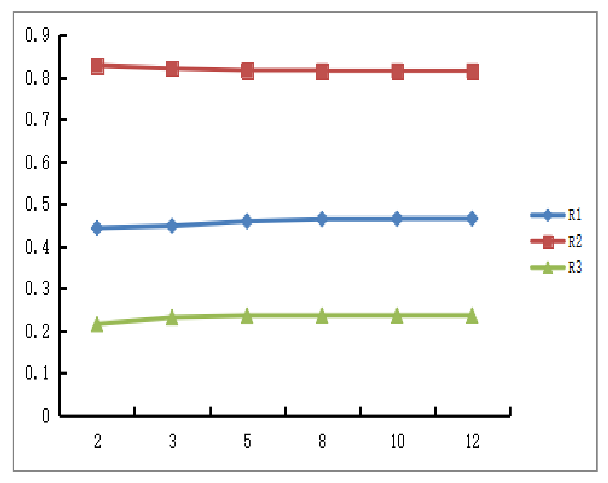
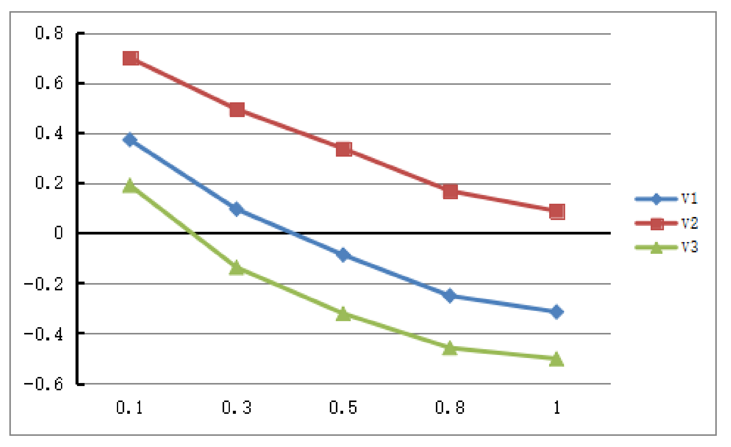
Next, we consider the relationship between the decision conclusion and the change of parameter λ. We still take the PLQROWA operator as an example. Assume $q=2,\alpha =\beta =0.88$, $\gamma =2.25$, and $\lambda =2,3,5,8,10,12$, respectively. The Figure 3 shows the corresponding ranking results (Table 9 shows the detailed calculation results). Obviously, the varies of value function $V_o$ is not sensitive to the parameter λ, which indicates that the parameter λ has little effect on the decision results.

Figure 3. The results of change λ in behavioral TOPSIS method.

Table 9. The detailed results of parameter λ.

	$\mathit{\lambda }=2$	$\mathit{\lambda }=3$	$\mathit{\lambda }=5$	$\mathit{\lambda }=8$	$\mathit{\lambda }=10$	$\mathit{\lambda }=12$
$V_1$	−0.2801	−0.2335	−0.2056	−0.197	−0.1957	−0.1953
$V_2$	0.1334	0.1078	0.0959	0.0929	0.0925	0.0923
$V_3$	−0.4797	−0.4052	−0.3806	−0.3768	−0.3763	−0.3761

5.3. Comparison Analysis with Existed Method

Here, the traditional TOPSIS method is used to compare with the behavioral TOPSIS method, the algorithm steps [29] are given as follow.

Step 1. Adjust the probability distribution of PLQRONs, the corresponding matrices $F^{(\ast 1)}$, $F^{(\ast 2)}$ and $F^{(\ast 3)}$ are obtained.

Step 2. Apply the PLQROWA operator to aggregate the evaluation information, then we normalize the aggregated decision matrix; the result is same as Section 5.2.

Step 3. Similarly, we can obtain the positive ideal solution $Q^{+}$ as follows:

$$\begin{array}{c}\hfill \begin{array}{cc}\hfill Q^{+}& =\{⟨\{s_0(0.5),s_{1.25}(0.1),s_{1.53}(0.2),s_{1.62}(0.2)\},\{s_{3.16}(0.3),s_{3.69}(0.2),s_{3.75}(0.2),s_{4.2}(0.3)\}⟩,⟨\{s_{4.27}(0.4),\hfill \\ & s_{4.6}(0.3),s_6(0.3)\},\{s_0(0.5),s_0(0.2),s_{1.41}(0.3)\}⟩,⟨\{s_{3.76}(0.3),s_{4.6}(0.1),s_{4.78}(0.6)\},\{s_0(0.7),s_{1.62}(0.3)\}⟩,\hfill \\ & ⟨\{s_0(0.5),s_0(0.5)\},\{s_{4.03}(0.3),s_{4.05}(0.4),s_6(0.3)\}⟩\}.\hfill \end{array}\end{array}$$

The anti-ideal solution $Q^{-}$ is also obtained as follows:

$$\begin{array}{c}\hfill \begin{array}{cc}\hfill Q^{-}& =\{⟨\{s_0(0.4),s_0(0.6)\},\{s_6(0.3),s_6(0.2),s_6(0.5)\}⟩,⟨\{s_{2.92}(0.5),s_{3.6}(0.1),s_{3.95}(0.4)\},\{s_0(0.1),s_0(0.3),\hfill \\ & s_0(0.1),s_{2.63}(0.5)\}⟩,⟨\{s_{0.9}(0.2),s_1(0.3),s_{1.85}(0.1),s_2(0.4)\},\{s_{2.26}(0.2),s_{2.77}(0.2),s_3(0.3),s_{3.27}(0.1),\hfill \\ & s_{3.78}(0.2)\}⟩,⟨\{s_0(0.5),s_0(0.5)\},s_6(0.3),s_6(0.2),s_6(0.5)\}⟩\}.\hfill \end{array}\end{array}$$

Step 4. If $q=2$, we apply $D_{ded}$ to calculate the distance of each alternative between $Q^{+}$ and $Q^{-}$, the results are obtained in Table 10.

Table 10. The separation measures for each alternative.

	${\mathit{Q}}_1$	${\mathit{Q}}_2$	${\mathit{Q}}_3$
$D_o^{+}$	0.1561	0.0549	0.2055
$D_o^{-}$	0.1236	0.2626	0.0561

Step 5. Calculate the closeness coefficient $R_o(o=1,2,3)$,

$$R_o=\frac{D_o^{-}}{D_o^{-}+D_o^{+}}.$$

By calculation, we get $R_1=0.4419$, $R_2=0.8271$ and $R_3=0.2145$. So the ranking order of the alternatives is $Q_2\succ Q_1\succ Q_3$. The decision result is same as behavioral TOPSIS method, which shows the proposed method is effective.

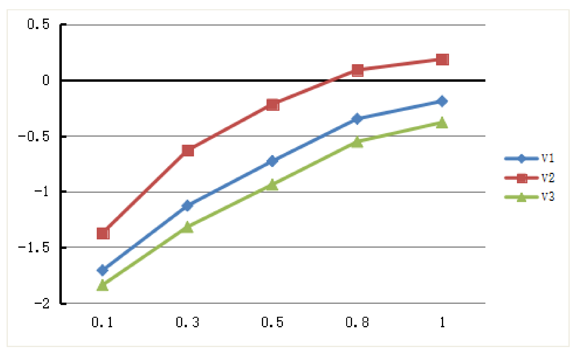
Similarly, we consider the relationship between the decision result and the change of λ based on the traditional TOPSIS method. Here $q=2,\alpha =\beta =0.88$ and $\gamma =2.25$, the parameter $\lambda =2,3,5,8,10,12$, we apply the PLQROWA operator to calculate the closeness coefficient $R_o$ of each alternative, Figure 4 shows the ranking results (Table 11 shows the detailed calculation results). As can be seen from Figure 4, the closeness coefficient $R_o$ remains unchanged and the decision result is also tend to stable.

Figure 4. The results of change the parameter λ in traditional TOPSIS method.

Table 11. The detailed results with the parameter λ.

	$\mathit{\lambda }=2$	$\mathit{\lambda }=3$	$\mathit{\lambda }=5$	$\mathit{\lambda }=8$	$\mathit{\lambda }=10$	$\mathit{\lambda }=12$
$R_1$	0.4419	0.4472	0.4582	0.4635	0.4644	0.4647
$R_2$	0.8271	0.8202	0.8156	0.8142	0.814	0.814
$R_3$	0.2145	0.2306	0.2347	0.2349	0.235	0.2351

5.4. The Sensitivity of Decision Maker’s Behavior

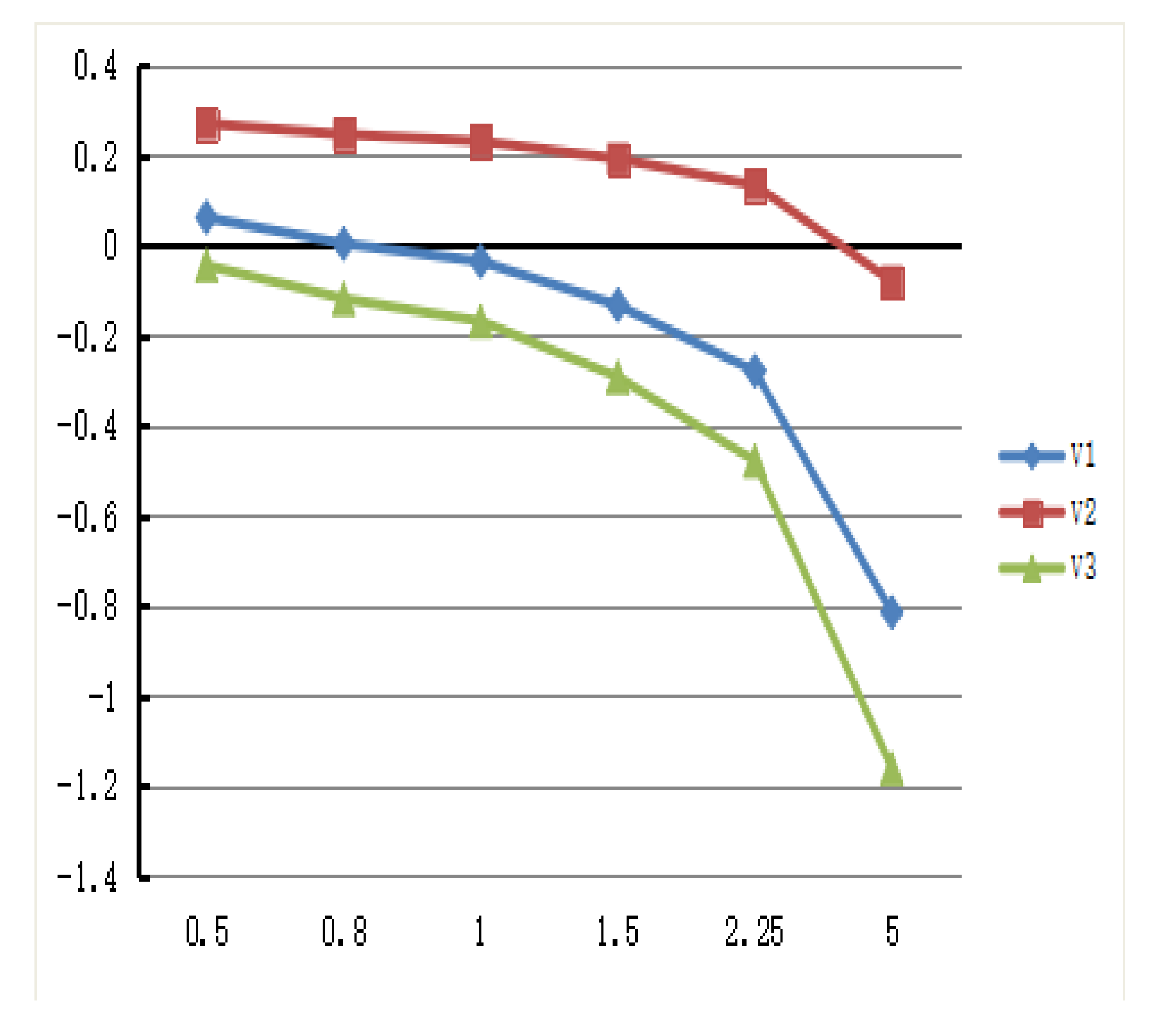
Here, we make the analysis of the influence of loss aversion parameter γ, the risk preference parameter α and β in the proposed behavioral TOPSIS method.

Firstly, the impact of the loss aversion parameter γ in the value function is considered. We take the PLQROWA operator as an example, if $q=2,\alpha =\beta =0.88$ and $\lambda =2$, let $\gamma =0.5,0.8,1,2.25,5$, the ranking results of the value function $V_o$ are shown in Figure 5 (Table 12 shows the detailed calculation results). As can be seen from Figure 5, when $\gamma \le 2.25$, the values of $V_1$, $V_2$ and $V_3$ are less sensitive to the change of the loss aversion parameter γ; while $\gamma >2.25$, the values of $V_o(o=1,2,3)$ is changing obviously. In comparison, the loss aversion parameter γ has a significant influence on $V_2$ and $V_3$. When $\gamma >2.25$, the values of $V_o(o=1,2,3)$ decrease sharply at the same time, which means if the parameter γ becomes larger, the loss aversion has a greater impact on the value function $V_o$.

Figure 5. The results of changed loss aversion parameter γ.

Table 12. Preference ranking under various loss aversion parameter γ.

	Distance Measure		Behavioral TOPSIS
			$\mathit{\gamma }=\mathbf{0.5}$		$\mathit{\gamma }=\mathbf{0.8}$		$\mathit{\gamma }=\mathbf{1}$		$\mathit{\gamma }=\mathbf{1.5}$		$\mathit{\gamma }=\mathbf{2.25}$		$\mathit{\gamma }=\mathbf{5}$
	${\mathit{D}}_{\mathit{i}}^{+}$	${\mathit{D}}_{\mathit{i}}^{-}$	${\mathit{V}}_{\mathit{i}}$	Rank	${\mathit{V}}_{\mathit{i}}$	Rank	${\mathit{V}}_{\mathit{i}}$	Rank	${\mathit{V}}_{\mathit{i}}$	Rank	${\mathit{V}}_{\mathit{i}}$	Rank	${\mathit{V}}_{\mathit{i}}$	Rank
$Q_1$	0.1561	0.1236	0.0613	2	0.0028	2	−0.0362	2	−0.1338	2	−0.2801	2	−0.8167	2
$Q_2$	0.0549	0.2626	0.2695	1	0.2461	1	0.2306	1	0.1917	1	0.1334	1	−0.0805	1
$Q_3$	0.2055	0.0561	−0.0449	3	−0.1195	3	−0.1691	3	−0.2934	3	−0.4797	3	−1.1629	3

Next, we consider the influence of the risk preference parameters α and β in the value function, respectively. We take the PLQROWA operator as an example, suppose that $q=2,\beta =0.88$ and $\gamma =2.25,\lambda =2$, let $\alpha =0.1,0.3,0.5,0.8,1$, the results of value functions change with the parameter α are shown in Figure 6. It is easy to know that the values of the function $V_o(o=1,2,3)$ descend with the parameter α. We know $Q_2$ is always the best alternative from the Figure 6. If $\alpha >0.88$, the values of $v_o(o=1,2,3)$ also tend to stable.

Figure 6. The results of change the risk preference parameter α.

Furthermore, assume that $q=2,\alpha =0.88,\gamma =2.25$ and $\lambda =2$, let $\beta =0.1,0.3,0.5,0.8,1$, the results of value functions change with the parameter β are shown in Figure 7. Similarly, we know that the values of $V_o(o=1,2,3)$ increase with the parameter β, and the best alternative remains unchanged. If $\beta >0.88$, the values of $V_o(o=1,2,3)$ tend to stable. In conclusion, the change of value function $V_o$ is consistent with expert’s risk preference, if the expert is risk averse, the parameter α increases, he/she is more sensitive to the loss, and the overall value functions are decreasing. If the decision maker is risk appetite, when the parameter β increases, he/she becomes more sensitive to gains, the overall value functions are increasing.

Figure 7. The results of change the risk preference parameter β.

According to the above comparison analyses, we can find that the proposed method has the following advantages. First, the behavioral TOPSIS method implements the decision maker’s choice by adopting the gain and loss. Second, it has been demonstrated that the traditional TOPSIS method is a special case of the proposed behavioral TOPSIS method [23], while the behavioral TOPSIS method involves a wider range of situations. In addition, there are three parameters (α, β and γ) in the value function of $V_o$, the decision maker can choose the appropriate numerical value according to his/her risk preference and loss aversion, which makes the proposed behavioral TOPSIS method more flexible in practical application.

6. Conclusions

The main conclusions of the paper are given as follows:

(1)

The operations of PLQROS are proposed based on the adjusted PLQROS with the same probability. Then we present the PLQROWA operator, PLQROWG operator and the distance measures between the PLQROSs based on the proposed operational laws.

(2)

We develop the fuzzy behavior TOPSIS method to PLQROS, which consider the behavioral tendency in decision making process.

(3)

We utilize a numerical example to demonstrate the validity and feasibility of the fuzzy behavior TOPSIS method, and we prove the superiority of the method by comparison with the traditional TOPSIS method.

Next, we will apply the proposed method to deal with the multi-attribute decision making problems, such as the emergency decision, supplier selection and investment decision, etc.