1. Introduction
In this paper, the spread of COVID-19 is discussed with a particular focus on the application of the containment measures, referring to the Italian situation.
Officially defined as a pandemic in March 2020, the disease induced by the SARS-CoV-2 virus, called COVID-19, has influenced and changed human life all over the world [
1]. Some of its peculiarities represent a complication in the identification of the epidemic outbreaks; one of them is the significant number of asymptomatic subjects, able to infect other people. An additional interesting characteristic of COVID-19 is the asymmetric increase in the number of hospitalised patients with age; in fact, while for young people the virus is almost harmless, for the elderly population, especially in association with pre-existing pathologies, it is extremely dangerous; the mean age of patients dead in Italy for COVID-19 is 81, counting more than
deaths and over than 3 million infected patients [
2,
3,
4]. Moreover, the reasons for the asymmetric increase in cases and case fatality rate among countries are still not evident [
5]; after a deep analysis of various factors that could justify the differences among countries, it seems that the density of the population plays an important role, suggesting a fast implementation of active control measures (as quarantine, the tracking of infections and testing) and a low case fatality rate.
The virus spreads through individuals’ movements and the most effective containment measure is the reduction in contacts among people, from mild public recommendations to strict lockdowns, with the use of masks everywhere; no specific medication is available and in severe cases, oxygen support is required [
1]. For a fast recognition of the infection (and therefore to prevent the spread of the virus), suitable swab tests are performed on subjects who are suspected to have had a dangerous contact or before entering the hospital or starting some activities. For example, a swab test campaign has been promoted by some Italian universities for their students [
6].
Despite all the containment measures applied, three epidemic waves can be recognised after a year of pandemic and to date, the most dangerous has been the second one, in November 2020.
In a few months, some vaccines have become available and countries are trying to immunise their population as quickly as possible; in fact, after some initial problems with the supply of doses, the vaccination campaign has the ambition of immunising more than of the European population by the end of next summer.
Since the beginning of the pandemic, many researchers have focused their works on studying the evolution of the virus spread, trying to predict future trends in the number of infected patients, in order to adequately set up suitable containment measures. Nevertheless, the unknown diffusion of asymptomatic subjects makes the challenge very difficult [
7,
8]; a possible estimation of the number of non-diagnosed subjects has been obtained by testing entire (small) communities, such as the case of the Italian city of Vo’, one of the first studies of this kind [
7], or by means of serological test campaign, as the one conducted in Italy during the period May–July 2020 [
9], which evidenced a significant number of subjects (a mean value of
of the population, not equally distributed in the country) that were infected by SARS-CoV-2 during the first months of the pandemic without knowing.
Some papers have been devoted to the analysis of real data trying to determine the modalities of the spread among nations, as in the early work [
10], or in a homogeneous population [
11,
12,
13,
14]. In the latter paper, a quite rich model composed by eight different classes is proposed: in addition to the usual susceptible (S), exposed (E), infectious with symptoms (I) and recovered (R) compartments, there are also the groups of pre-symptomatic infectious (A), the hospitalised (H), the quarantined susceptible (Sq), the isolated exposed (Eq) and the isolated infected (Iq) compartments.
Due to the specificity of the virus, interesting works have focused on age-compartmental models, as in [
15], where the role of quarantined subjects is emphasised, referring in particular to residential care homes, or as in [
16], in which the initial contagion step was distinguished among age-classes.
Sometimes, previously studied models for other epidemic emergencies are adapted to the specificity of COVID-19, like in [
17], where a short time forecast is provided, on the basis of the few data initially available. On the other hand, the current COVID-19 emergency has been the inspiration for a more general analysis as in [
18], in which the problem of how to face the next wave of infectious disease is studied by analysing the global symmetries of the system under suitable time rescaling. It shows the importance of controlling the arrival of the next wave when the number of infections grows linearly, i.e., during the period between waves.
As already noted in the cited papers, the model structure that appears suitable to describe the COVID-19 evolution inside a population is the one (referring to the four classes of subjects in which the population is partitioned: Susceptible–Exposed–Infected–Removed), enriched with the classes specific for this emergency, like the asymptomatic individuals and the quarantined ones.
All the proposed models must consider the containment measures applied since the beginning of the pandemic, including social distancing, the use of masks, medication, the swab test, informative campaigns and the vaccination. In [
19], the importance of using masks is studied, even in the case of non-totally effective protection; it models both the inward and outward efficiency of the mask, disaggregating the population variables into those that do and do not use masks. The results show how the use of masks decreases the effective transmission rate, especially with other interventions, such as social distancing and hygienic measures. In particular, social distancing and informative campaigns are discussed in [
20,
21]. The social distancing measure is modelled by means of a nonlinear function influencing the contact rate; numerical simulations show the impact of this specific containment measure on the virus spread. The importance of general awareness in regard to the dangers of COVID-19 infection was investigated in [
21], in which the impact of the media campaign is studied, along with the rapid testing; the class of susceptible individuals is partitioned depending on the careful application of preventive behaviours, and the test campaign was modelled by improving the transfer of subjects from the asymptomatic (and dangerous) condition to the infected diagnosed one.
The identification of the model is therefore influenced by these actions, the consequences of the governments’ choices and of personal behaviours; as previously mentioned, the strict lockdown is the most effective action to contain the spread. Nevertheless, it cannot be the solution for long periods, for both social and economic reasons; therefore, there have been attempts to propose proper and balanced containment measures, depending on the evolution of the pandemic [
22]. It is worth noting that awareness of the impact of the containment measures can also modify people’s behaviours and therefore the trend of pandemic itself.
In this paper, starting from the model proposed in [
23], the problem of identifying the applied containment measures is faced, studying the model under the realistic condition of the implementation of these actions since the very beginning of the health emergency. The consequence is the possibility of identifying the restrictions as they were really applied by the population and by the healthcare system, observing on one hand an increase in the awareness of people in the application of social distancing (also depending on the specific period under study) and, on the other hand, a general improvement in the capability of the sanitary system to face the emergency. This identification, corresponding to a sort of transducer of the government’s measures, is useful when one wants to predict what would happen by applying the same kind of control measures already applied or a combination of them.
The paper is organised as follows; in the second section, the mathematical model was recalled and studied, determining the equilibrium points, the effective reproduction number and discussing the identification of the containment measures by proposing a suitable cost index. In the numerical results section, after showing the effectiveness of the identification procedure as well as the fitting ability, interesting scenarios are studied.
2. Materials and Methods
In this section, the mathematical model proposed in [
23] is enriched with the introduction of the possible control actions, the test campaign, the quarantine, the medication and the vaccination, as shown in
Section 2.1. The model is studied in
Section 2.2 and
Section 2.3, determining the equilibrium points and proposing a stability analysis, calculating the expression of the basic reproduction number and studying its relation with the equilibrium points. In
Section 2.4, the identification of the applied containment measures is proposed.
2.1. The Mathematical Model Proposed and Introduction of the Containment Measures
In the model adopted and briefly recalled in this subsection, all the typologies of controls that can be put in place for containing the spread of COVID-19 and for the reduction of its mortality are introduced. The state space dimension is kept as low as possible to maintain the simplicity and immediacy of a SEIR model, but including those classes specific to the main characteristics of COVID-19, thus allowing to determine the effects of the controls introduced. The six-dimensional system proposed is:
where:
S is the class of susceptible individuals;
E is the class of infected patients in the incubation phase; they cannot infect other subjects;
is the class of the infected patients without symptoms; they are infective and then are responsible for the disease spread. They can remain asymptomatic for all the illness course or can start to have some symptoms;
is the class including the diagnosed infected patients which are isolated and then cannot transmit the virus even if infective. Patients in this class are the ones that can receive medical treatment both for the infection and for secondary diseases or complications;
Q is the class of the suspected infected individuals which are temporarily isolated and tested for positivity of the SARS-CoV-2, or simply quarantined for security reasons;
R is the class of the recovered individuals, the ones which healed spontaneously or after therapy, which are supposedly no longer infected.
The parameters introduced in (
1)–(
6) have been extensively described in [
23]. The death rates in each class are denoted by the
terms. The constant rate
B of new incoming individuals was only added in the susceptible class, considering the negligible time of permanence in the other classes with respect to the population growth. Parameter
is the contact rate. The parameters
k,
,
and
denote the natural transition rates between classes;
b and
c are related to the results of the tests on the suspected cases in
Q. More precisely,
b is the rate of return from quarantine of the supposedly healthy people, while
c denotes the rate of transition from
Q to the class corresponding to the results of the test, healthy with probability
(test negative), or infected for the remaining
, defined according to the average time required for the tests.
As far as the control actions , , are concerned with reducing the spread of the virus and to take care of medical issues, respectively, the following functions are introduced:
, with an efficacy coefficient a, which denotes the action aiming to stimulate or force a test campaign on the population, even without any suspect of infection. The goal is to recognise infected individuals as early as possible to reduce the contact rates;
models the isolation indications, aiming to reduce the interaction with other people. This isolation acts on the factor for the part responsible of the frequency of individual contacts; it is bounded between zero and one, with corresponding to an ideal total individual isolation;
represents the therapy action devoted directly to counteract the virus by means of antiviral drugs; the associated coefficient denotes the effectiveness of the therapy;
is the therapy action aiming at reducing the side-effects, typically the induced cardio–respiratory diseases. Its effect is introduced as a direct contribution to reduce the mortality rate and it is bounded between zero and one, corresponding, respectively, to no therapy and to the desirable condition of all individuals kept alive during the course of the infection;
models all the constraints (medical, political and economical) influencing the tests policy and the consequent effects;
regards the vaccination strategy, possible since the end of 2020. The coefficient v denotes the efficiency of the vaccination, depending on the individual response and on the type of vaccine used.
2.2. Model Analysis
In this section, the qualitative analysis of the system behaviour is proposed, choosing to include the control actions , ; the reason for this is that it can be assumed that there is a lack of any containment measure only in the very first period of the epidemic, until January 2020, when nobody, at least in Europe, was sufficiently aware of the danger of the situation.
Aiming at the unified analysis in which all potentially active control actions are naturally included in the system evolution, the following positions are assumed:
=
=
=
= +
=
=
=
Moreover, for the sake of simplicity in the formulation, the following non-negative functions are introduced:
= + +
= +
= + + +
=
= + +
= +
The model analysis was performed, as usual, by assuming constant controls
, which correspond to constant values for
; the equilibrium points are determined by equating the second members of the Equations (
1)–(
6) to zero, that is, by using the notations introduced above, by solving the system:
Observing that in absence of infection,
(being equal to 1 the probability of having negative COVID-19 test), it is easily verified that the disease-free equilibrium (
), always present, is given by
once the solution with
is taken. Note that, as will be used later, when
, the following identity holds
.
A second equilibrium point:
the endemic one, can be found in (
7)–(
12). In particular, from (
9) and (
8), it can be obtained that:
By substituting in (
11), it results:
and
is obtained, as function of
, from (
10):
All these quantities, with the exception of
, definitely depend on
, and are well defined once
is defined. Its expression is obtained from (
7) by
This solution can be accepted only if positive; by substituting the definitions of
,
, it can be easily shown that the denominator is always positive, whereas the sign of the numerator depends on the condition:
The meaning of the herein defined expression
will be discussed in the next subsection, when determining the
Effective Reproduction Number [
24].
As far as the analysis of the stability property of is concerned, the following result can be stated.
Proposition 1. The disease-free equilibrium point is asymptotically stable if and only if: In fact, by writing the Jacobian of the controlled system (
1)–(
6) and using the introduced notations with the
quantities, it is obtained that:
Due to the special structure of the Jacobian
J, its characteristic equation evaluated in
has two negative roots,
and
, found considering the sixth and the fourth columns; the other roots are obtained from the four degrees polynomial:
whose coefficients
,
contain the defined quantity
previously introduced:
To study the sign of the real part of the roots of the
, Routh’s arguments are used [
25]; first of all, it can be noted that, since
,
, it results that the sign of the
is the same as
, as it can be easily shown by substituting the definitions of
,
in
, always positive. By applying Routh’s rule to
, the sign of the two quantities must be studied:
From the definitions (
24)–(
27), and substituting the expressions of
,
, it can be deduced that they are positive if
. Therefore, it is possible to conclude that in this case, the disease-free equilibrium is stable. When the second equilibrium point exists, see condition (
20), the point
becomes unstable.
2.3. The Effective Reproduction Number
As already stated, the model analysis is performed assuming constant controls, thus obtaining the equilibrium points that depend on those values of the containment measures. In the contest of coping with the pandemic, these actions are generally kept constant for a period of at least two weeks, to be able to see their effects and provide suitable adjustments of the containment measurements, if needed. In this sense, both and (when the latter equilibrium point exists) depend on the applied controls, and therefore, on the period during which the chosen actions are applied. The , , in particular, has a special meaning; if a population is in that condition by means of the (constant) control actions introduced during a specific period and for the model parameters, and if the quantity is positive, then the evolution of the population will remain near , without allowing the spread of the epidemic. Referring to COVID-19 (and therefore assuming fixed model parameters) and to the definition of , a suitable application of social distancing (thus acting on ), of swab tests and quarantine (thus acting on and ), medication (acting on ) and vaccination (control ) would lead the population to the .
The quantity
introduced in (
20) is related to the
effective reproduction number, the actual average number of secondary cases per primary case at calendar time
t [
26]. More precisely, this indicator, when evaluated in absence of any control action (i.e., at the beginning of the epidemic), is the well-known
, the
basic reproduction number that can be estimated from data or by using the
next-generation matrix approach [
24,
27].
The introduction of the containment measures aims to reduce the incidence of the epidemic; in this case, the
effective reproduction number is an indicator of the epidemic evolution and of the effectiveness of the applied control actions. Generally, it is determined from data, that by using a statistical approach [
28], or by adapting the previously cited
next-generation matrix approach, as proposed in [
24,
29,
30]. The difference between the methods proposed in the above-cited papers relies on the points in which the next-generation matrix is evaluated; according to the approach in [
30], the reproduction number will be herein evaluated by using the disease-free equilibrium (
13), which includes the vaccination, when possible, and the tests campaign, with all controls assumed constant when the
evaluation is performed.
The computation starts by considering in the dynamics (
1)–(
6) the classes directly involved in the spread of infection,
E,
,
and
Q, and therefore only the Equations (
2)–(
5). By using the notations with the
,
quantities, the reduced system (
2)–(
5) may be written and enhance the contributions due the infection,
, and the ones due to changing the health condition,
:
The variations of these vectors with respect to the variables
E,
,
and
Q, evaluated in the disease-free equilibrium, yield the matrices
F and
V, respectively:
and:
Under these positions, the effective reproduction number is given by the dominant eigenvalue of the matrix
, given in this case by its
element; its computation easily yields the same expression defined in (
20),
.
Therefore, also in the proposed approach that includes the control actions, it can be deduced that if the effective the reproduction number is smaller than 1, there exists a unique equilibrium point, the disease-free equilibrium one that is stable; otherwise, the equilibrium points are two and the disease-free one is no longer stable.
2.4. Containment Measures Identification
The approach adopted in this paper was to consider the model evolution influenced by the application of the containment measures since the very beginning of the analysis; this is reasonable as the data only started to be collected at the end of February 2020 with the introduction of measures of increasing severity [
1]. All the actions
,
, are assumed between 0 and 1. Note that for the controls, the value 0 corresponds to the absence of any action, whereas 1 represents the maximum effort. The controls are multiplied by factors representing the effectiveness of the control; therefore, the identification of the containment measures is obtained once the evolutions of the quantities
,
,
,
,
and
are determined. Note that the meaning of the evolution of
is opposite with respect to the corresponding one of
: when the control
is maximum (ideally equal to 1), the quantity
has its minimum value (corresponding to the absence of contacts); similar consideration holds for the control
and the quantity
.
The data that will be used for identification regard the Italian situation; they were downloaded from the Civil Protection website [
2]. More precisely, there are considered:
The number of newly diagnosed infections obtained considering the sum of the variation of the number of infected patients, of the recovered and the deaths between two consecutive days; is the corresponding quantity evaluated from the model;
The number of positive patients corresponding to the ones of this model;
The number of subjects officially recovered
from COVID-19, corresponding to:
The number of patients deceased from direct effects of the virus—
—corresponding to the following function obtained from the model:
The number of subjects vaccinated with the two doses corresponding to the quantity of the model.
The following cost index is proposed, aiming to fit the available real data, by minimizing the errors between measured quantities and the corresponding outputs of the model:
where the parameters
,
weight the relevance of each term in the optimisation procedure.
All the available information will be used to improve the numerical identification of the quantities
,
,
,
,
. For example, it is well known that the vaccination campaign only started in January 2021; therefore, in the first period, it could be assumed
. Another possible simplification regards the relation between the two controls
and
. In Equation (
4), the two contributions related to healing and to death are assumed to be separated since they correspond to different therapy actions. Nevertheless, in some ways, they refer to the same kind of resources, referring to the medication aspects; therefore, for the sake of simplification, to better match the real data available, it can be reasonably assumed that there is a relation among
and
:
where parameter
is related to the rate of healing for infected patients. This implies that a simplified choice for the cost index (
34) can be assumed, leading to the identification of
,
,
up to the end of December 2020, with the addition of
starting from January 2021.
3. Numerical Results
In the model introduced in
Section 2, the parameters can be distinguished on the basis of their dependence on the characteristics of the considered population or of those of SARS-CoV-2. Difficulties in this system identification arise from different causes. One is related to the real data collection; especially during the first period of the pandemic, when the data were not collected as a consistent modality, not even in the same nation. Moreover, the importance of retrieving some information was not evident since the beginning of the emergency; also, the official communication of the updated numbers of infected patients or of dead subjects was in some cases delayed, thus producing unexpected spikes, hardly predictable, in the corresponding data evolution. Another difficulty in the identification is related to the non-measurability of the important category on asymptomatic subjects (the ones modelled in the
class) and consequently, of the total removed ones in
R.
Moreover, it is worth stressing what inspired the approach of this work: that is, the presence of control actions since the very beginning of data collection. During the period considered, of March 2020–April 2021, different and complementary containment measures were adopted by all governments all over the world, without coordination among nations, at least at the very beginning.
In the following, the main containment measures at the Italian national level are summarised, indicating the period of application:
From 23 February 2020 to 8 March 2020: introduction of increasing measures aimed at containing the diffusion in the north of Italy;
From 9 March 2020 to 25 April 2020: strict lockdown in the entire nation; all the “non-essential” activities were suspended, distanced learning was introduced for both schools and universities, and whenever possible, smart working was introduced. It was possible to leave home only for emergencies. This period was called “Phase 1”;
From 26 April 2020 to 10 June 2020: almost all activities started again, but it was not possible to travel between regions. This period is “Phase 2”;
From 11 June 2020 to 12 October 2020: it was the period with less restrictions, even with the suggestion of preserving cautions; it was also allowed to travel, always respecting social distancing; this was the “Phase 3”;
From 13 October 2020 to 2 November 2020: introduction of increasing containment measures common to all the nation with restaurants closed at 18:00 and a mandatory use of masks also outside closed places;
From 3 November 2020 to 21 December 2020: a curfew from 10 p.m. to 5 a.m. was introduced; moreover, a classification mechanism was adopted, classifying each region into three classes indicated by colours (yellow, orange, red) depending on the diffusion of the virus and on the sanitary situation at territorial level. Briefly speaking, in this phase of colours, the red condition corresponds to a strict lockdown, with restriction in personal mobility also inside the cities; in the orange situation, it was not possible to move among regions with bars and restaurant open only for take-away. In the yellow regions, bars and restaurants were open until 18:00; teaching was allowed at schools/universities with restrictions on the number of students allowed in classrooms;
From 22 December 2020 to 6 January 2021: the strategy based on the colours was reinforced; all of Italy was at the orange level, but these became red on the day before and after the 25 and 31 December and 6 January, respectively;
From 7 January 2021 to 30 April 2021: the strategy with colours during the period 3 November–12 December was adopted with reinforced rules, making it more difficult to pass from a higher danger level, red and orange, to the lower one, orange and yellow, respectively.
This representation of the control actions applied by the Italian Government, as well as their time scheduling, is of course simplified; the consistency of the evolutions of the control actions identified will be discussed considering the real control actions.
As mentioned previously, some model parameters could be chosen on the basis of medical information or related to the characteristics of the population, as can be seen in
Table 1 for the numerical values of the fixed model parameters and the corresponding references. Note that the values referring to the medical characteristics of the disease must be considered mean values, also depending on the generally healthy condition of the patient.
The other parameters of the model can be identified by minimising the cost index (
34) or a simplified version, if (
35) is assumed, thus yielding the evolutions of
,
,
,
,
and indirectly, of
. The corresponding non-controlled constant values
a,
,
,
c and
can be deduced, if needed, from the first values of the quantities with the bar sign, recalling that the controls
,
are assumed between 0 and 1. By using the @Matlab software and the function
fmincon, the fitting between real data and the model output was performed. The minimisation of the cost index during the period February–December 2020 was obtained, after a
trial and error procedure, with the following choice of the weights:
,
,
, with
, being the vaccination campaign not started at that time; from January 2021, the weights are chosen as equal to
,
,
,
. In
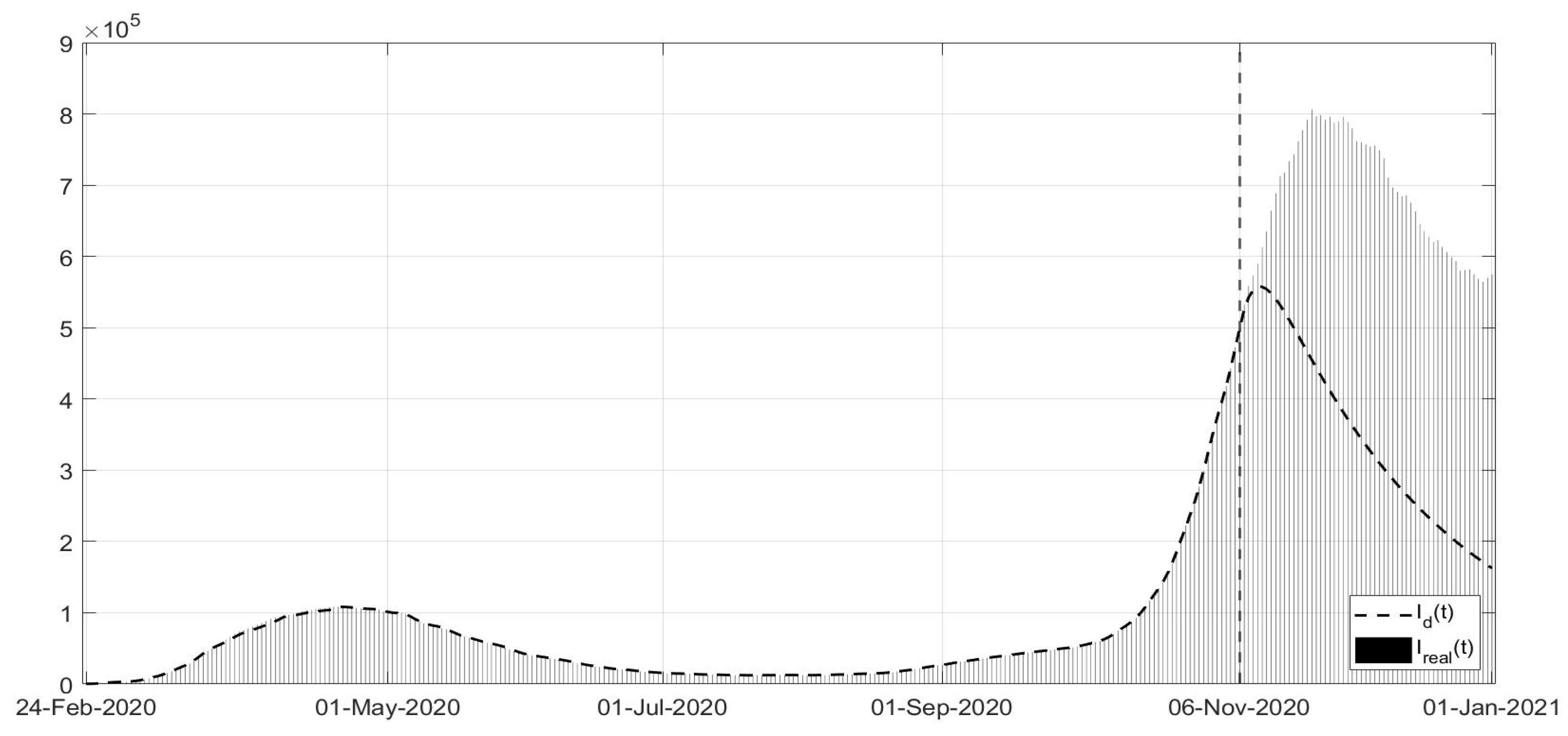
Figure 1,
Figure 2 and
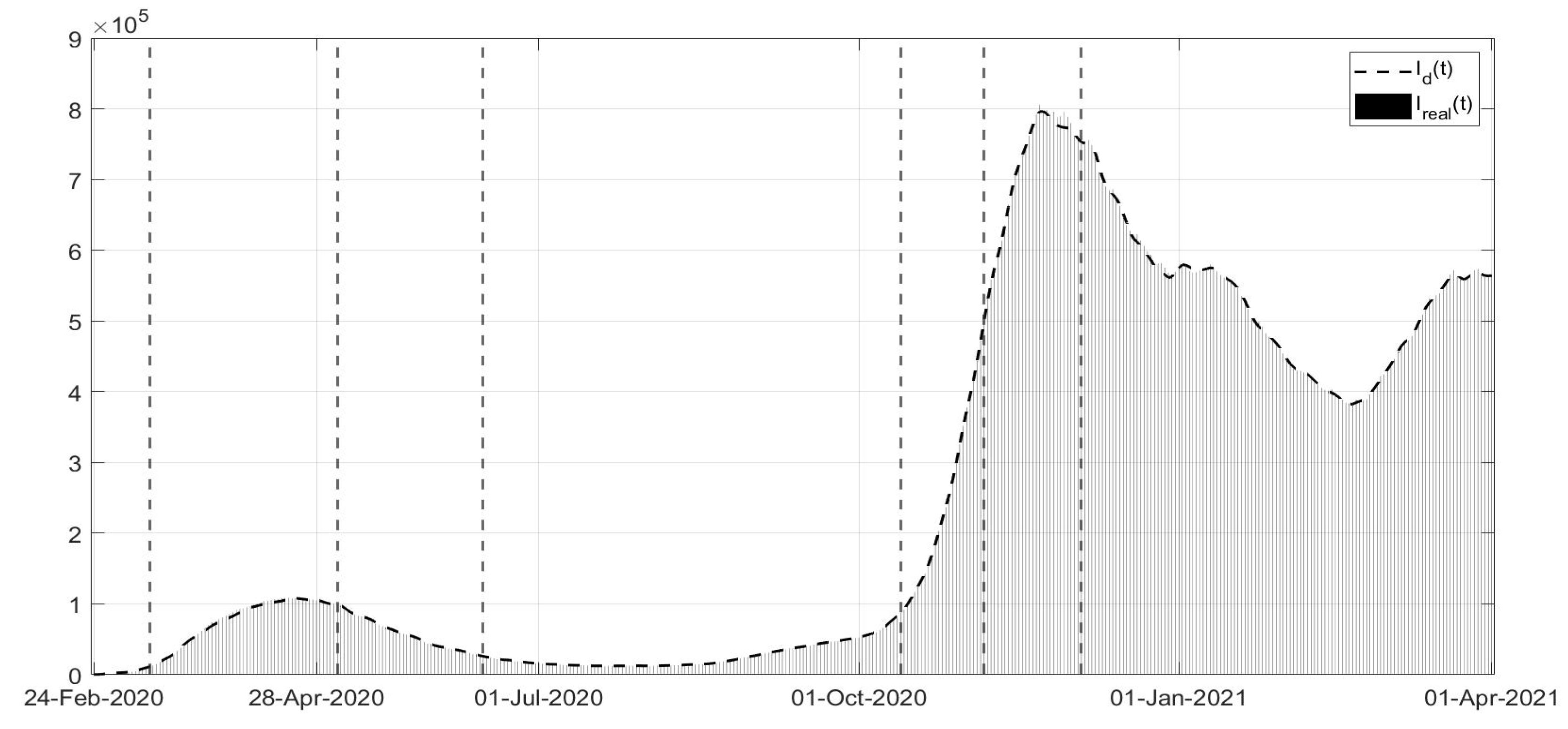
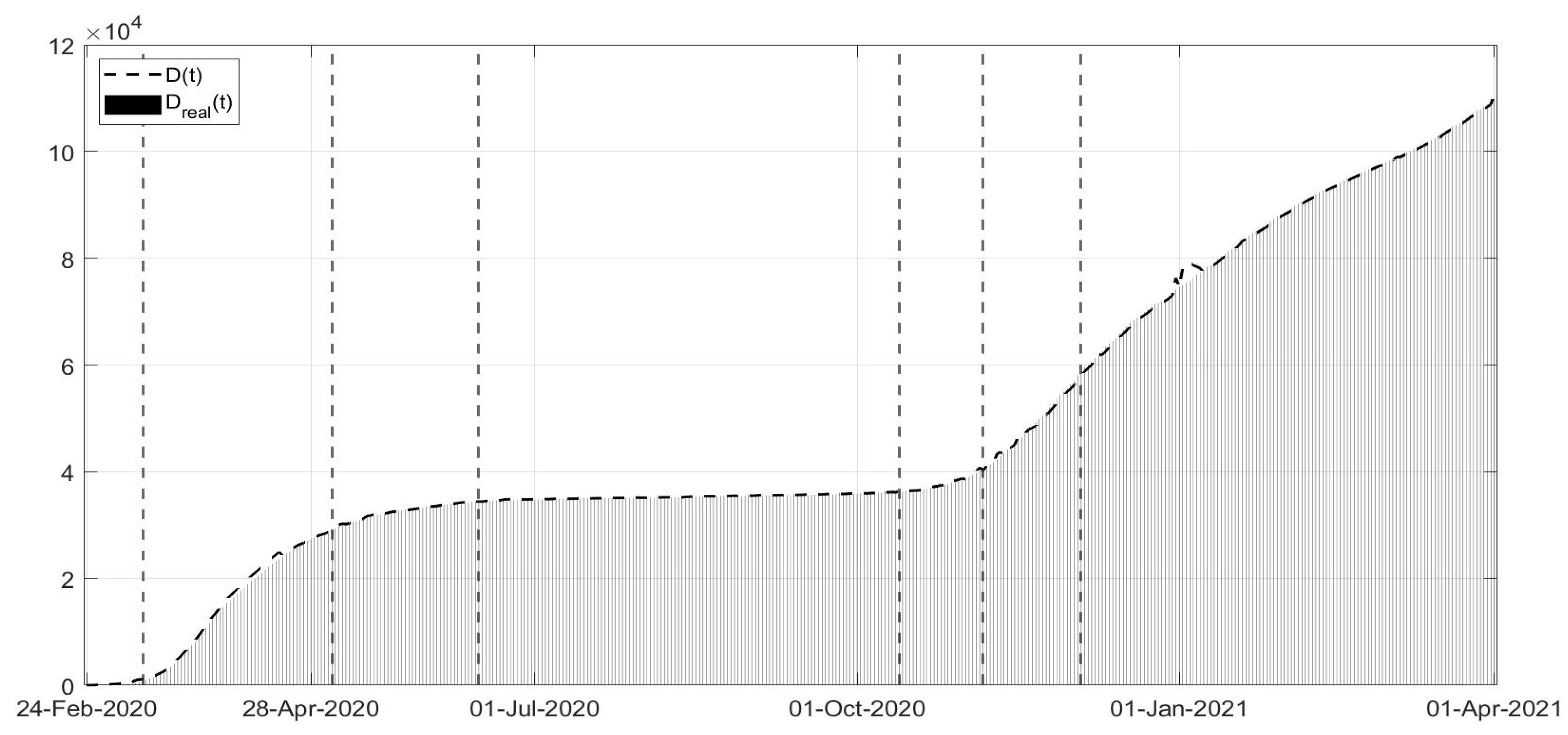
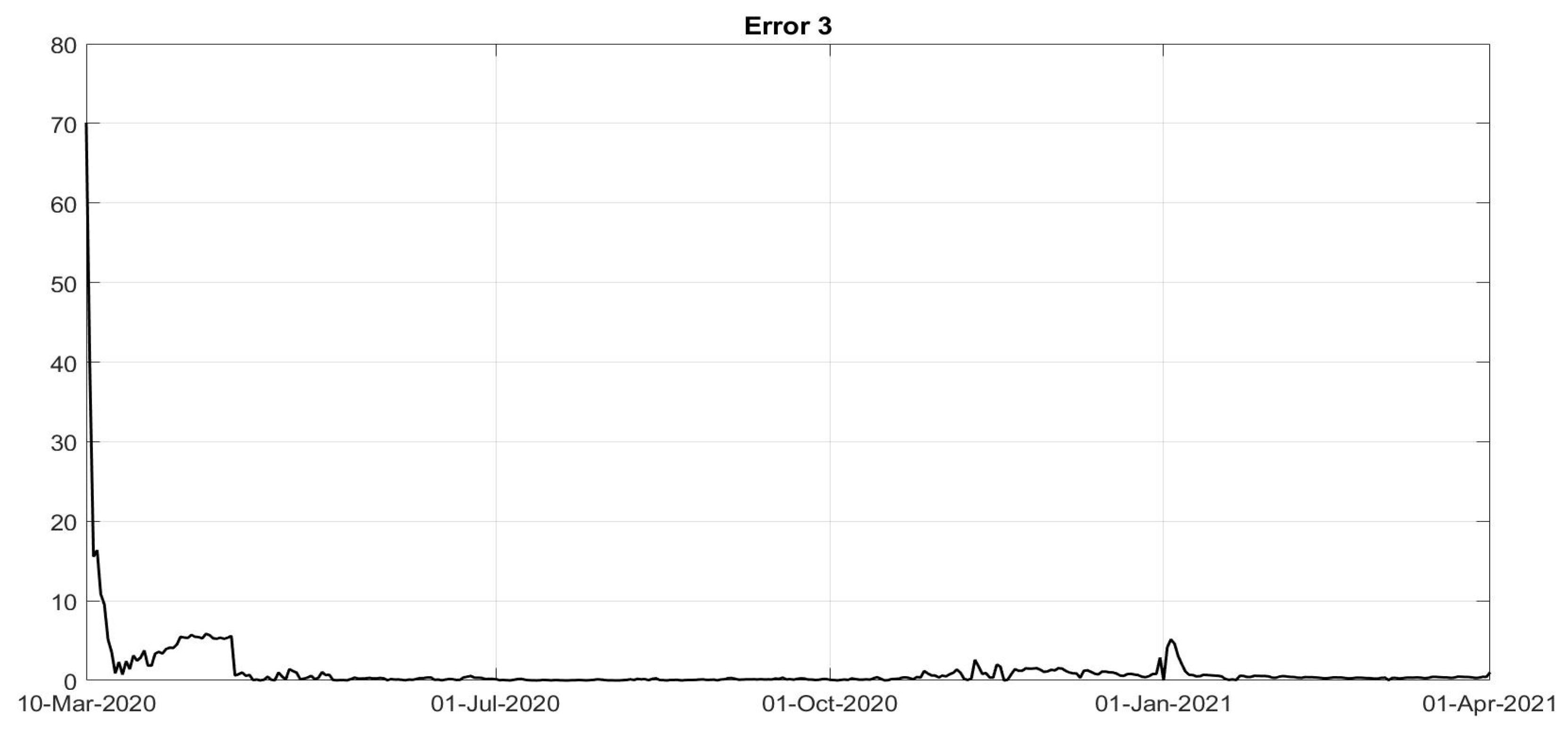
Figure 3, the evolutions of the diagnosed infected patients, of the recovered individuals and of the dead subjects are shown along with the corresponding real data; a good fit can be appreciated, in some way overcoming the not completely satisfactory data collection of the first period of the pandemic; in particular, in
Figure 1, the three waves of pandemic can be noted, in April 2020, in November 2020 and March 2021. In
Figure 4,
Figure 5,
Figure 6,
Figure 7 and
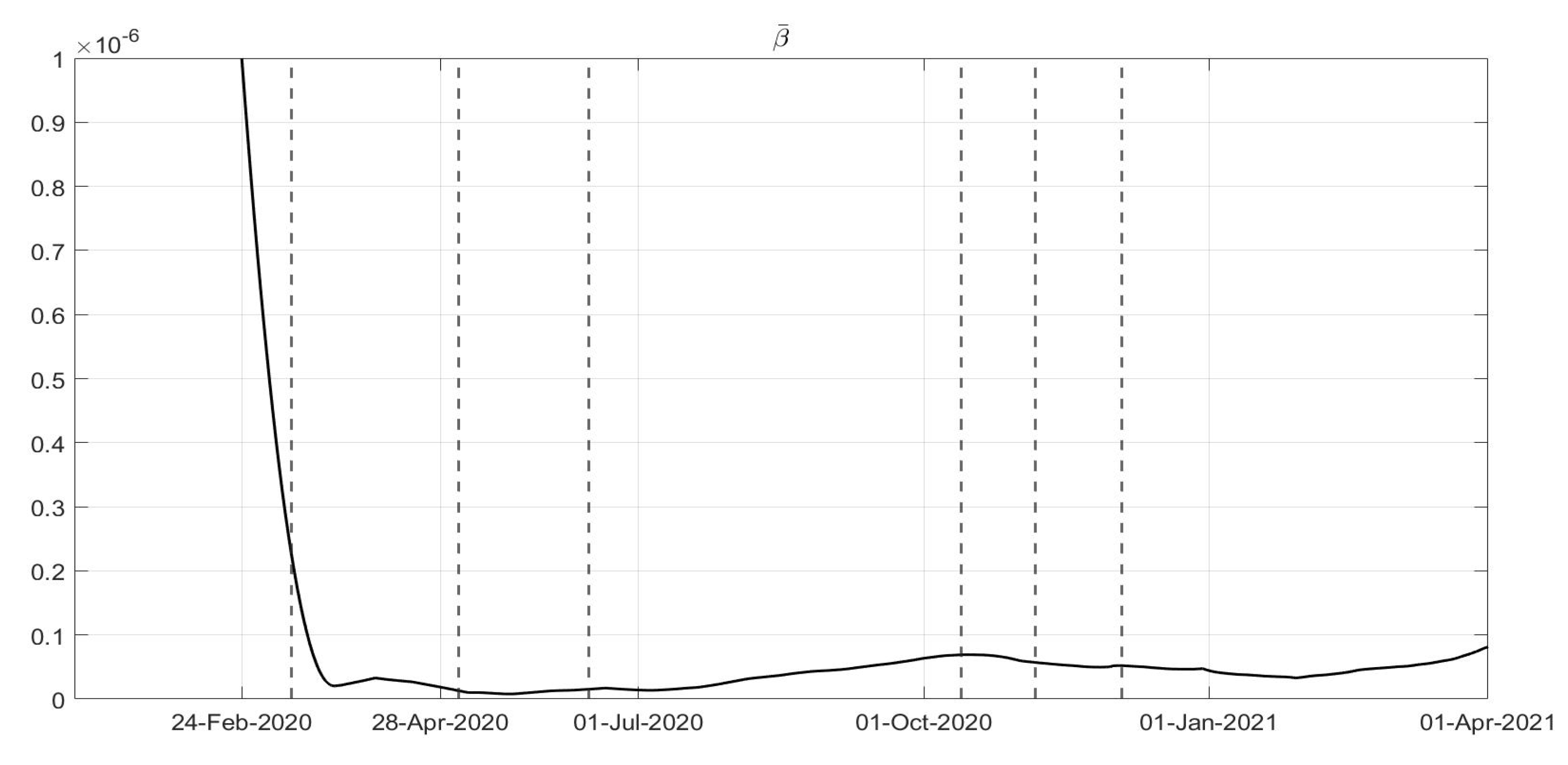
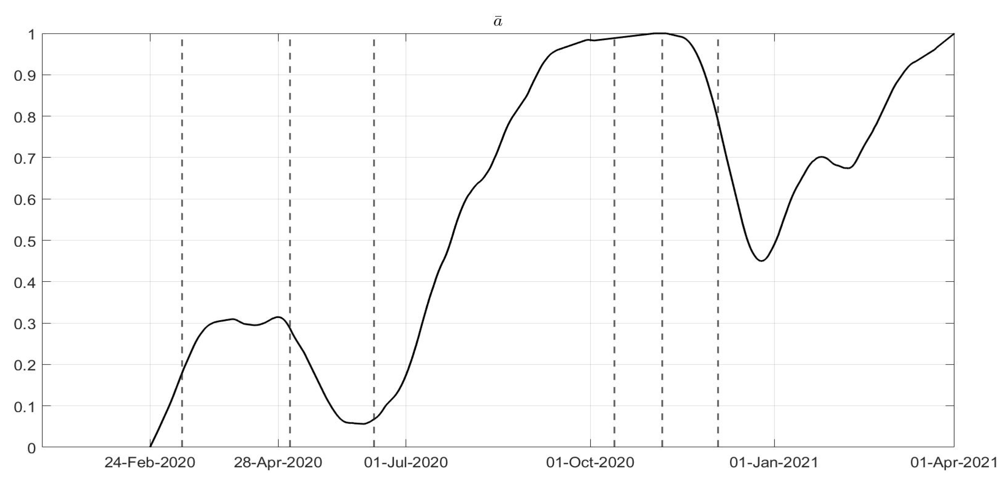
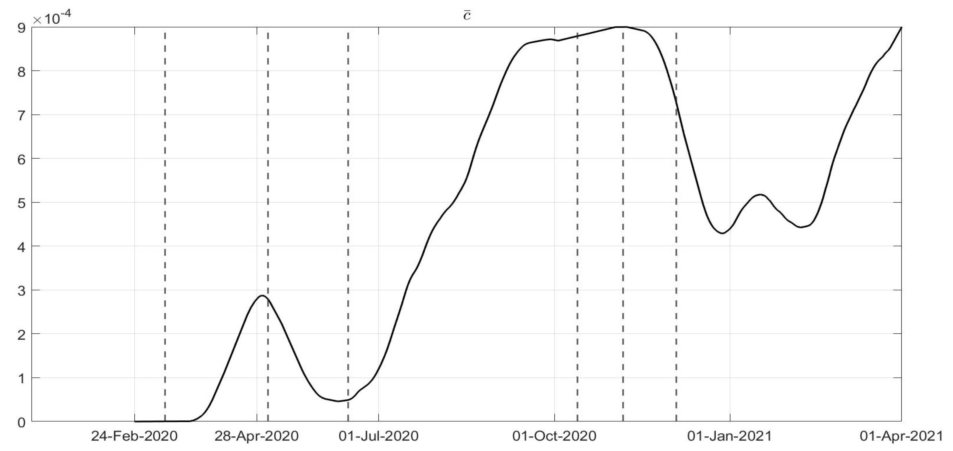
Figure 8, the identified control actions are shown; in each figures the dotted vertical lines correspond to the significant changes in the adoption of the containment measures previously recalled. Particularly interesting is the evolution of
in
Figure 4: a general decrease in the evolution of
can be noted until July, due to the effects of the strict lockdown of Phase 1; then, an increase can be noted until the middle of October, with the re-opening of schools and of many activities. New increasing containment measures were then applied with the “phase of colours” starting in November, thus obtaining a decrease in the values of
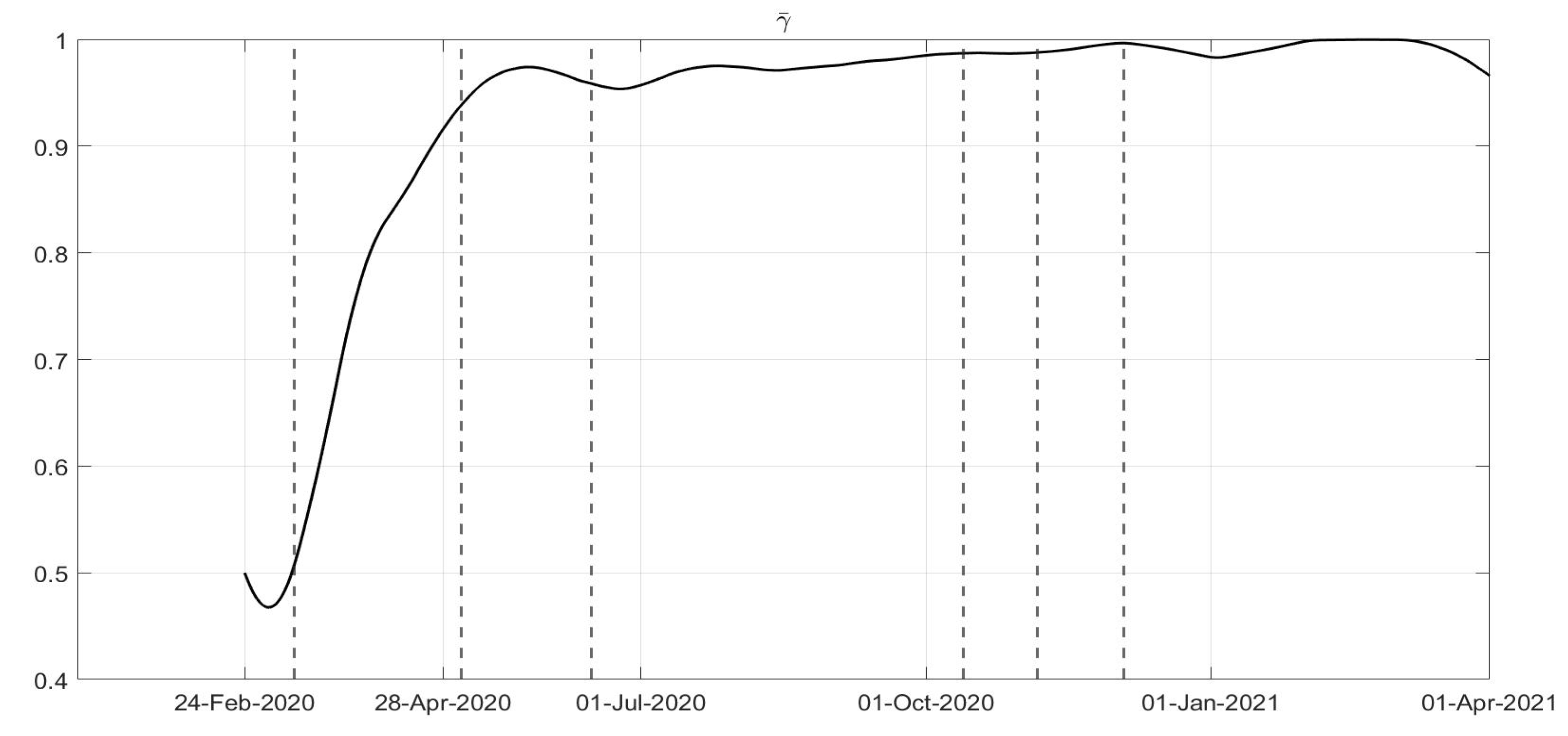
until March. The evolutions of
and
are quite similar, as shown in
Figure 5 and
Figure 6, corresponding to an increase in the capability of isolating subjects for a quarantine period and the improvements in the swab testing, respectively, with two decreasing periods in June 2020 and December 2020. As far as the
evolution is concerned as desirable, it has been increasing since the very beginning of the pandemic, showing a general resilience capability in the sanitary system, as shown in
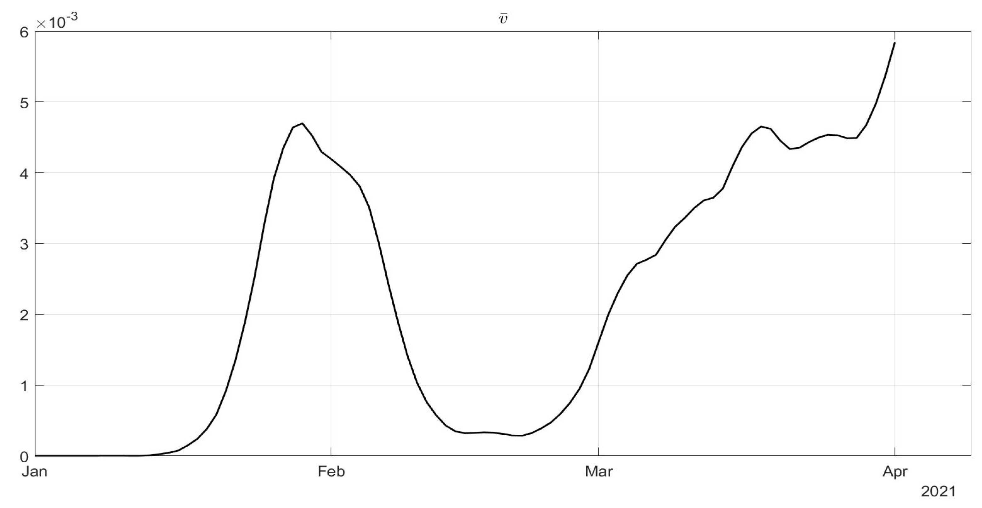
Figure 7. The vaccination action, represented by
, only started in January 2021; its evolution, to date over less than three months, shows an oscillatory increase until the middle of February, and then an increasing trend, as shown in
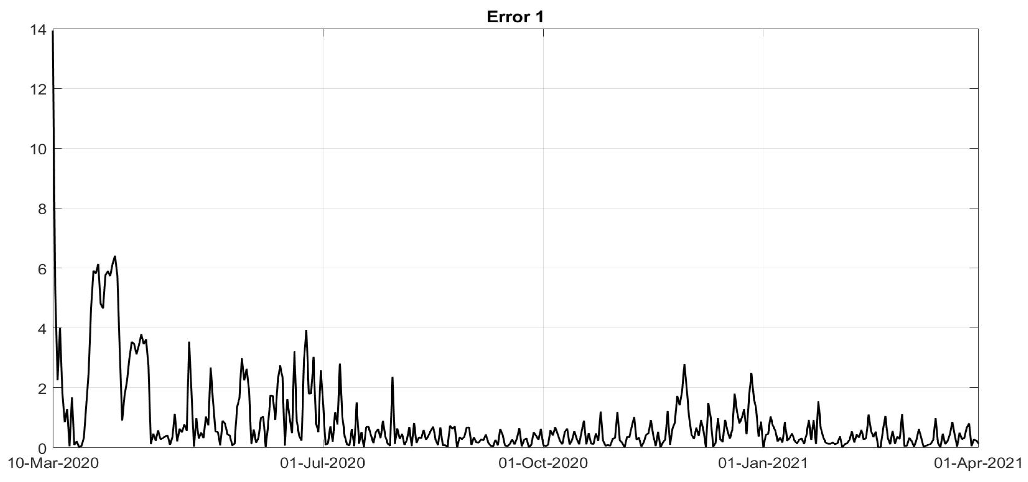
Figure 8. To evaluate the goodness of the identification step, the evolutions of the percentage of the normalised errors, in absolute values, indicated, respectively, with
Error 1,
Error 2 and
Error 3, between the real numbers of diagnosed infected patients, of recovered individuals and of deaths and the corresponding quantities obtained from the model, are shown in
Figure 9,
Figure 10 and
Figure 11. Note that, after the first few days of the identification period, the maximum error was always less than
and in general, after July, less than
. The identification of the evolutions
,
,
,
is important since it allows to determine a connection between the decisions about the containment measures and how they have been applied by the population; for example, the strict lockdown of Phase 1 was not applied by the population as an
on–off control: it required some weeks to adapt to the new condition. Therefore, on the basis of this consideration, it is possible to study some scenarios determining what could have happened if different choices were made. Five scenarios are considered:
Scenario 1: Instead of the applied containment measures (phase of colours), the adoption of the strict lockdown was assumed, starting in November 6; the trends of
,
and
were obtained using the evolution of the
identified during the lockdown period (
Figure 4);
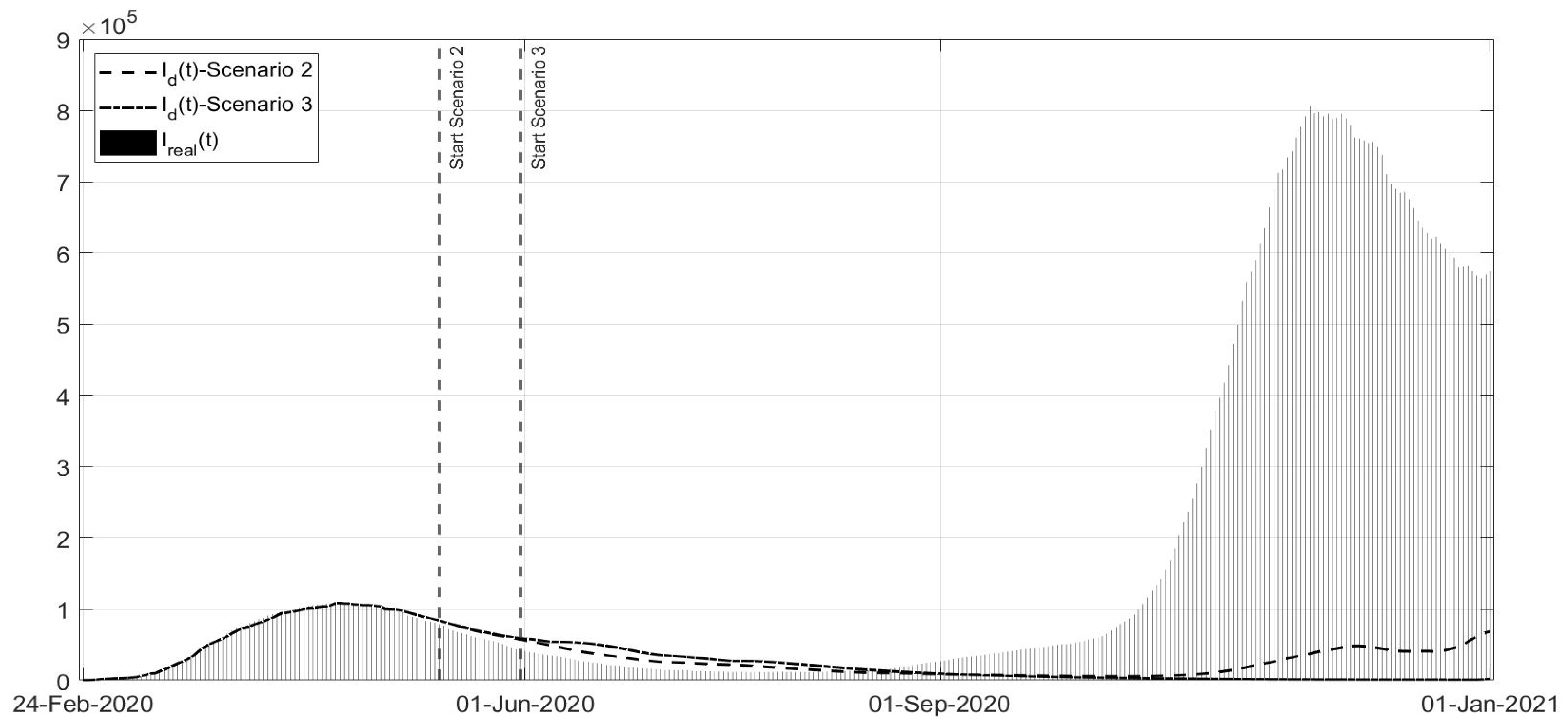
Scenario 2: Instead of ending the strict lockdown at the beginning of May 2020, it is hypothesised that there was an extension until 13 May;
Scenario 3: Same as Scenario 2, but with the extension of the strict lockdown until 31 May;
Scenario 4: Regards the vaccination campaign associated with different containment measures from 14 March 2021; in this scenario, it is assumed that the strict lockdown associated with the higher vaccination effort was already applied at the end of January;
Scenario 5: Same as Scenario 4, but the containment measures applied were those of November 2020 (phase of colours).
In Scenario 1 (
Figure 12,
Figure 13 and
Figure 14), it is evident that there is fast decrease in the number of infected patients in
Figure 12, and deaths in
Figure 14; obviously, the number of recovered subjects also decreases, as shown in
Figure 13, having less patients to heal. Therefore, the adoption of a strict lockdown starting in 6 November 2020 implies a more efficient measure in contrasting the virus spread with respect to milder actions, avoiding many victims, more than 9000. In general, the choice of the containment strategy takes into account different goals and constraints, including social and economic requirements, that in this paper are not considered (
Figure 12,
Figure 13 and
Figure 14).
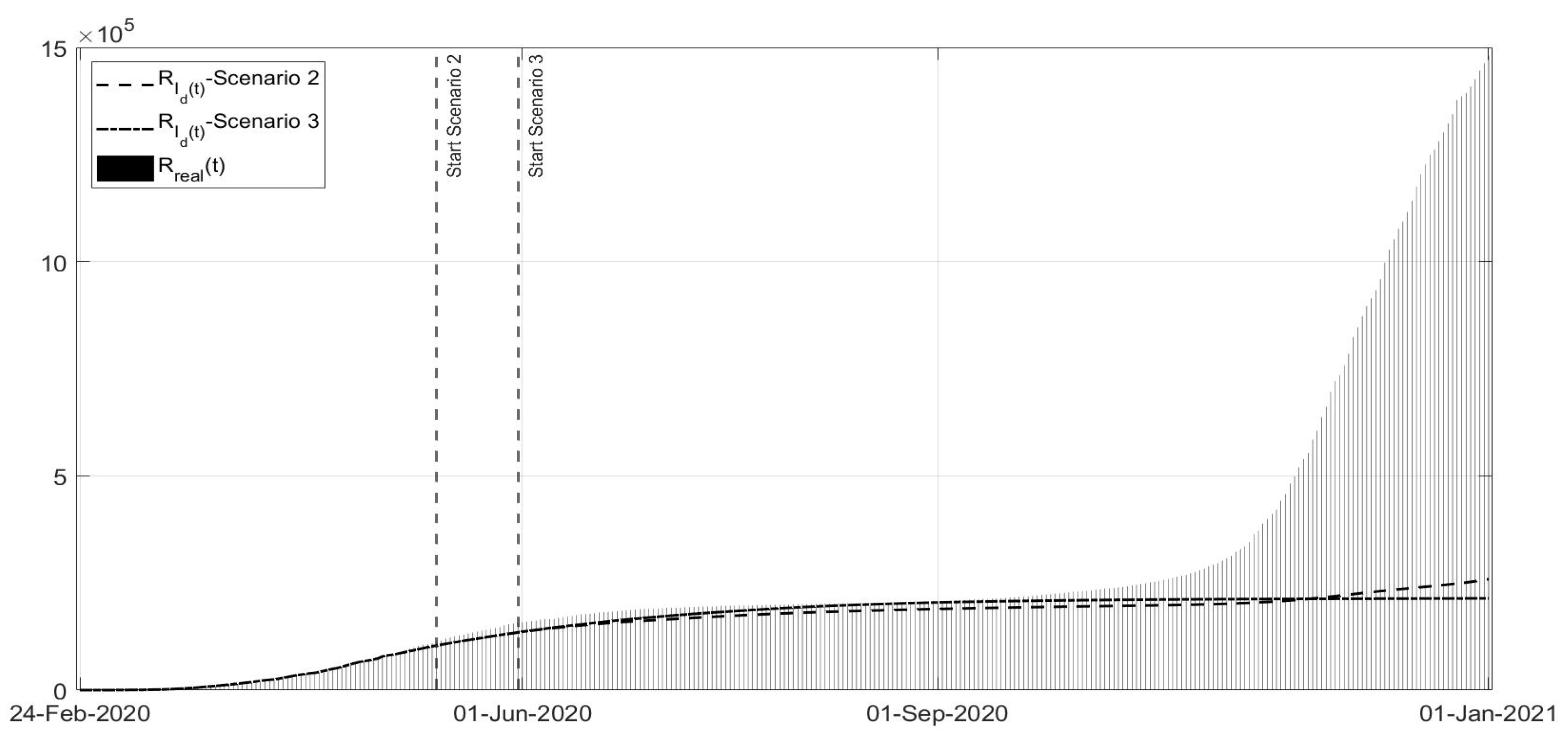
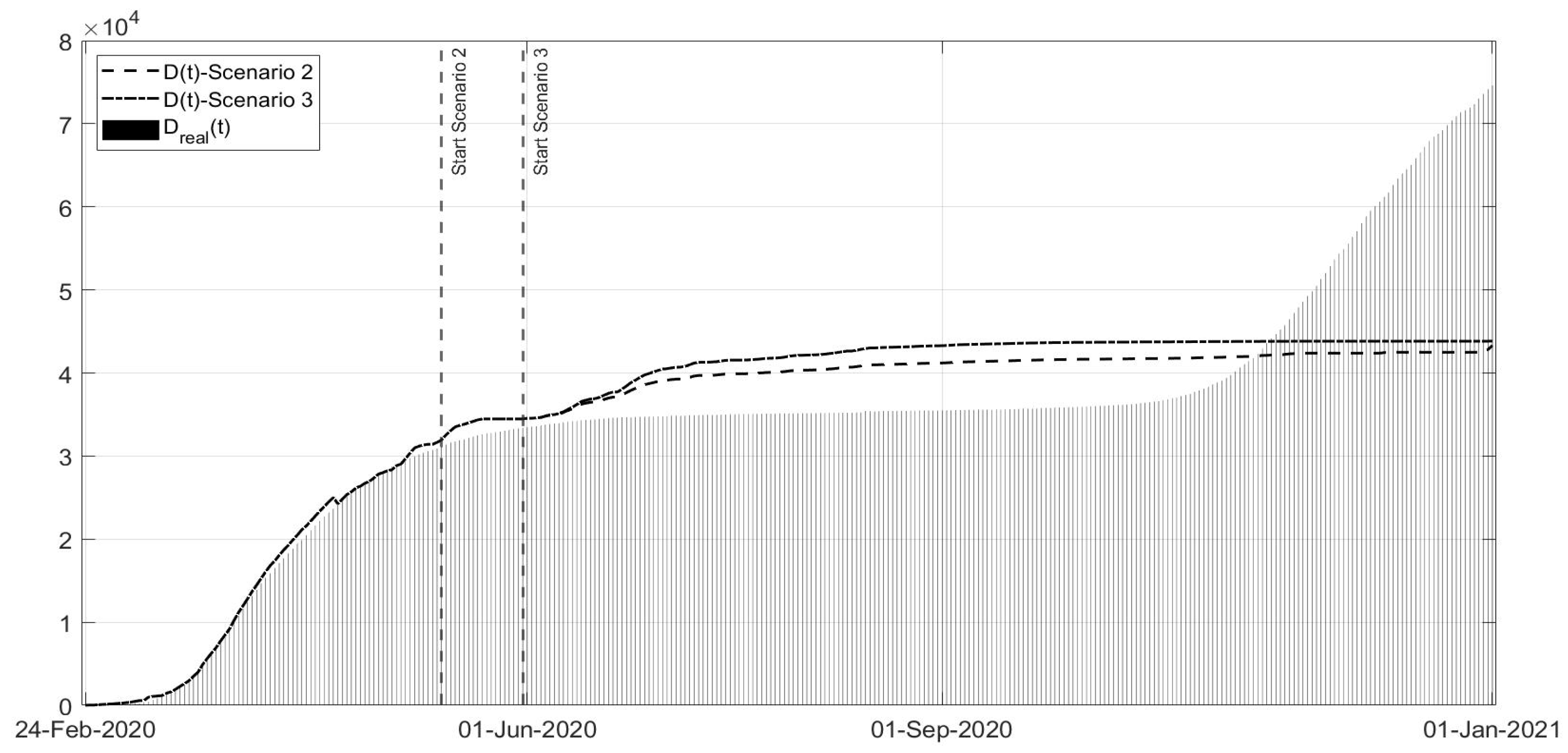
Scenarios 2 and 3 are studied together, as shown in
Figure 15,
Figure 16 and
Figure 17; they regard the decision of ending the strict lockdown of Phase 1 not at the beginning of May 2020 (as really happened) but in the middle and at the end of May, respectively. It can be noted that, also with an extension of only two weeks of Phase 1 restrictions, the peak of the second COVID-19 wave would have been sensibly lower also with respect to the peak of the first wave. The number of deceased patients remains almost constant in these scenarios, sensibly lower when compared with the real evolution. The results are evident especially in the Scenario 3, if the Phase 1 would have been extended until the end of May. These scenarios confirm the importance of stabilising the infection curves at low levels before re-opening; for example, in Australia, the current approach is even to apply the strict lockdown also with a few dozen cases. Due to the high contagiousness of SARS-CoV-2, it was observed that the increase in the general trend of infected patients was faster than the decrease due the containment measures and to lower the curve requires stronger effort as the number of infected patients is higher.
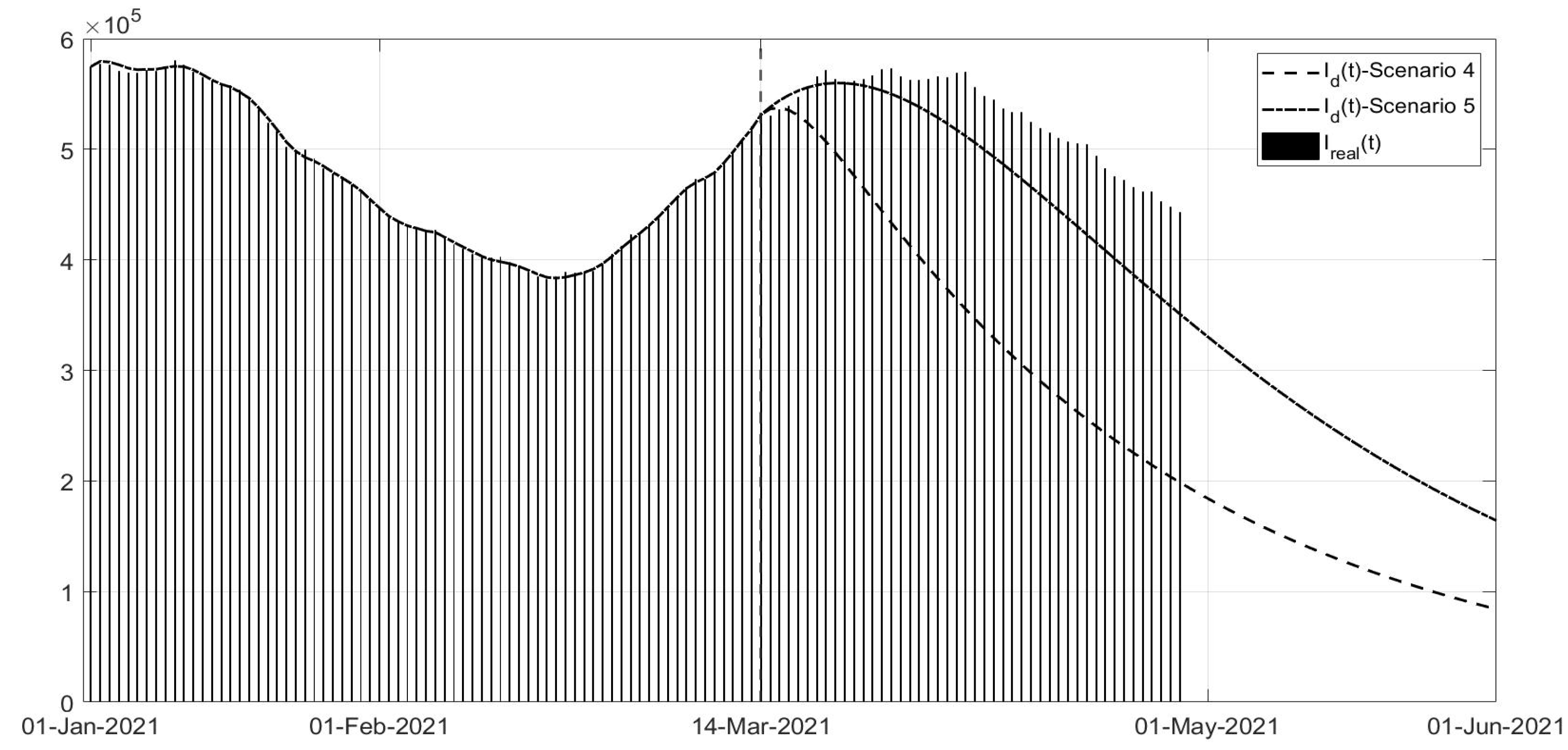
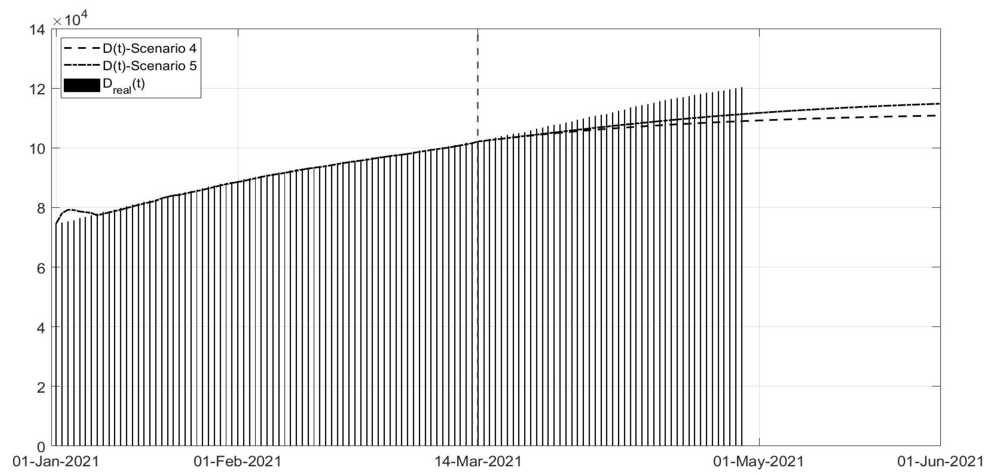
Scenarios 4 and 5 regard the management of the vaccination phase,
Figure 18,
Figure 19 and
Figure 20; all governments are trying to accelerate the vaccination campaign, in the meantime limiting the spread of virus to avoid the development of new variants. In some cases, such as in the UK, the vaccination campaign was associated with a strict lockdown obtaining a rapid decrease in the number of infected patients and deaths. In Scenario 4, a fast decrease in the number of infected patients can be noted, whereas the application of the phase of colour containment measures, shown in Scenario 5, yields a less evident decrease in the infections,
Figure 18. In particular, the simulation results in
Figure 18,
Figure 19 and
Figure 20 were compared with the real data representing what is currently happening; it can be observed that the currently applied containment measures allowed a decrease in the number of new infections, slower than in the simulated scenarios, probably also for the new unknown variants of the virus. Nevertheless, it must be stressed that, as seen, any new action or behaviour influences the evolution of the spread, and in particular, the number of infected patients. The increased number of infected patients implies an increased number of deaths, as can be seen in
Figure 20.
From the analysis of these scenarios, it can be confirmed that a severe reduction in mobility strongly reduces the infection; the effects are even more evident when the contact reduction is associated with a fast vaccination campaign; nevertheless, social and economic considerations are influencing, as expected, the decisions about containment measures, often in contrast with the suggestion of epidemiologists.
4. Conclusions
The reduction in the impact of COVID-19 in terms of the number of infected patients and deaths depends on the choice of containment measures, from the strict lockdown to vaccination, possibly applied in a coordinated way. Mathematical modelling allows to describe the epidemic spread, introducing all the controls available until now. In this paper, referring to the Italian pandemic conditions, taking into account some of the peculiarities of COVID-19, a suitably enriched model is proposed, including the effective control actions available to date. Considering the real data regarding the number of infected patients, deaths and vaccinated subjects, the main result of the paper consists in the identification of the applied control actions, enabling a direct correlation between the government’s decisions, as they were really applied by the population, and the numerical evolution of the functions representing the control actions. By means of this identification, the estimated effects of the containment measures, associated to the different periods of the pandemic, could be used to study the possible scenarios, in order to understand the effects of different choices, and their impact, also suggesting time scheduling and severity. In particular, the advantages of strict measures have been evidenced, such as those of the lockdown, that, while difficult for the population and the economy, could have accelerated the reduction in the spread. The importance of studying the possible scenarios depending on different control actions relies on the consideration that in a globalised world, a pandemic is not an exception and mutatis mutandis, the experience of facing COVID-19 should be useful in similar situations. Future developments regard the possibility of studying the effects of re-infection after vaccination and/or after being infected and healed; the proposed model and approach could be useful to determine the best control actions, also considering the new information about the available vaccines, the duration of the immunity, and specific medication.


